| Issue |
A&A
Volume 693, January 2025
|
|
|---|---|---|
| Article Number | L21 | |
| Number of page(s) | 4 | |
| Section | Letters to the Editor | |
| DOI | https://doi.org/10.1051/0004-6361/202453058 | |
| Published online | 27 January 2025 | |
Letter to the Editor
A Bond albedo map of Europa
1
Université Paris-Saclay, CNRS, GEOPS, 91405 Orsay, France
2
Institut Universitaire de France (IUF), Paris, France
3
Aurora Technology BV for ESA, Noordwijk, Netherlands
⋆ Corresponding author; This email address is being protected from spambots. You need JavaScript enabled to view it.
Received:
18
November
2024
Accepted:
8
January
2025
Abstract
Context. Europa’s surface is globally highly reflective, but it shows significant spatial variations in albedo. Accurately estimating Europa’s energy balance would require mapping the surface’s bi-directional reflectance distribution function albedo. However, this quantity is challenging to observe and model across all viewing and illumination angles and all locations on the moon.
Aims. This study aims to generate a comprehensive Bond albedo map of Europa at the highest spatial resolution possible to support the detailed thermal and photometric analyses essential for interpreting surface conditions.
Methods. We present a new approach to creating an absolute Bond albedo map of Europa using photometric data and high-resolution imagery. The Bond albedo was determined for 20 regions of interest (ROIs) based on Voyager and New Horizons data using Hapke parameters. By correlating these values with the average pixel intensities for each ROI on the USGS map, we determined a linear relationship between the Bond albedo and pixel intensity.
Results. This linear correlation allowed us to extrapolate a Bond albedo map across Europa’s surface with spatial resolution matching the United States Geological Survey mosaic. The resulting map provides a valuable dataset for energy balance assessments and can be used in detailed thermal modeling of Europa’s surface for upcoming missions. This product may also be useful for optimizing captor exposure times.
Key words: techniques: photometric / planets and satellites: fundamental parameters / planets and satellites: surfaces
© The Authors 2025
 Open Access article, published by EDP Sciences, under the terms of the Creative Commons Attribution License (https://creativecommons.org/licenses/by/4.0), which permits unrestricted use, distribution, and reproduction in any medium, provided the original work is properly cited.
This article is published in open access under the Subscribe to Open model. This email address is being protected from spambots. You need JavaScript enabled to view it. to support open access publication.
1. Introduction
The Bond albedo, sometimes also called the spheric albedo, planetary albedo, or bolometric albedo, refers to the fraction of power from the incident Sun radiation that is scattered back out into space by an astronomical body. It includes all the photons reflected in all directions and from all illumination directions (at all local times) at a given location of the planet. In practice, it is very hard to measure this quantity without a dedicated instrument either on the ground or from space because of the difficulty to complete all geometric measurements.
On the other hand, the production of high-resolution maps is governed by the fusion of images taken from multiple flybys at various effective surface resolutions, illuminations, and viewing angles. An empirical photometric correction is often applied, resulting in a very useful mosaic for photo-geological purposes and context maps, but not for quantitative photometry.
There is currently no Bond albedo map of Europa publicly available in the literature. Rathbun et al. (2010) produced an albedo map for some regions of Europa using thermal data inversion; however, due to the limited coverage of the Photopolarimeter-Radiometer (PPR) instrument, ∼80% of the surface remained unmapped. Trumbo et al. (2018) also derived the Bond albedo through a photometric approach with a linear relationship, but their method relies solely on Voyager data and uses the normal albedo, which does not capture the full reflectance properties of the surface. Moreover, neither their dataset nor their linear relationship is publicly accessible.
Building on this approach, we propose rescaling the global United States Geological Survey (USGS) map (Becker et al. 2010) to get an estimation of the Bond albedo using local anchor points. Unlike Trumbo et al. (2018) and Buratti & Veverka (1983), who relied on normal reflectance, our method uses local photometric data obtained from several regions of interest (ROIs).
2. Data
2.1. USGS grayscale mosaic of Europa
The USGS map1 (Becker et al. 2010) serves as a reference to identify pixel intensities for each point on Europa, as shown in the background of Fig. 1. This global map incorporates the highest-resolution and moderate-resolution coverage available from the Galileo Solid-State Imaging (SSI) instrument and the Voyager 1 and 2 missions. The map is projected on a spherical model of the mean radius of Europa, 1562.09 km. It should be noted that a data gap exists at the south pole, where no coverage is available below latitude −83°, and that only low-resolution data are available for the north pole and various high-latitude areas in both hemispheres.
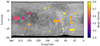 |
Fig. 1. 20 ROIs overlaid on the USGS map, annotated with their corresponding average Bond albedo values derived from Hapke parameter analysis. Longitude is expressed according to the west-increasing definition. |
This dataset relies on the visible spectrum, which captures most of the Sun’s energy but not near-infrared wavelengths. Although Europa appears bright in visible light, it becomes darker in the near-infrared due to water ice absorption, which could lead to a slight overestimation of the Bond albedo in our method and in Trumbo et al. (2018).
2.2. Local photometry of ROIs
Belgacem et al. (2020) derived individual photometric parameters for 20 different ROIs using a combined Voyager and New Horizon visible imaging dataset (represented as rectangles in Fig. 1). They used the semi-infinite monolayer model of the Hapke model (Hapke 2012a), as described in Belgacem et al. (2020). This widely used spectro-photometric model describes the reflectance of a planetary surface as a function of the observation geometry and a few physical parameters: the single scattering albedo (ω), the particle phase function, the macroscopic roughness of the surface, and the opposition effect. Since the geometries in this work are far from opposition, this last term is neglected.
Although most of the areas were consistent with the typical backscattering already identified on Europa, this work showed a significant variability of the photometric properties across the surface. In particular, it highlighted the established dichotomy between the albedo of the leading and trailing hemisphere, but it also identified surprising behaviors. For instance, it pinpointed areas with strong forward-scattering that could be indicative of fresh activities, such as plume deposits. It also showed how diverse the estimated macroscopic roughness could be, reaching values as high as 26°. The description of the different ROIs and the individual photometric parameters are detailed in Tables 2 and 3 of Belgacem et al. (2020), as well as in their Supplementary Materials. Overall, they emphasize the importance of studying photometry at different scales and deriving appropriate models.
3. Methods
3.1. Bond albedo of ROIs from Hapke parameters
To derive the average Bond albedo of the ROIs from the photometric parameters obtained in Belgacem et al. (2020), we applied an analytical approach based on the Hapke model (Hapke 2012a).
In the case of isotropic scatterers, instead of performing a numerical integration of the reflectance for all angles, the Bond albedo can be retrieved directly using an analytical solution, as shown by Hapke (2012b, see their Eq. 11.19). Following van de Hulst (1974), to account for anisotropic scattering, we modified the Bond albedo expression by replacing γ with  , where ω* = 2cω/(1 − ω + 2cω) and c is the fraction of backscattered light (from fully forward-scattering, c = 0, to fully backward, c = 1). Using similarity relations from Hapke (2012a) in the case of scatterers described by their average backscattering fraction (c), this leads to the expression of the Bond albedo:
 (1)
(1)
For each ROI, we retrieved the mean single scattering albedo (ω) and the mean backscattering fraction (c) and their uncertainties from Tables 2 and 3 of Belgacem et al. (2020). We then used Eq. (1) to compute the mean Bond albedo of each ROI, as shown in Fig. 1 superposed on the USGS map.
We chose to exclude ROI number 18 from this study because it is a poorly constrained region with the largest photometric parameter errors. Specifically, the two key parameters ω = 0.88 ± 0.04 and c = 0.78 ± 0.22 have significant uncertainties (Belgacem et al. 2020). The unusually large uncertainty in ω is particularly suspicious, raising doubts about the reliability of the data in this region (Souchon et al. 2011; Schmidt & Fernando 2015).
3.2. Pixel intensity to Bond albedo
To obtain a high-resolution map of the Bond albedo, we assumed that there is a linear relationship between the Bond albedo and the pixel intensity of the USGS map:
 (2)
(2)
where α and β are fitting parameters and Ip(λ, φ) is the intensity (between 0 and 255) of the pixel found at latitude λ and longitude φ on the USGS map.
The ROIs serve as anchor points for fitting this linear relationship. Since each ROI covers a different area, we selected all pixels within its region on the USGS map and calculated the average pixel intensity to compare it with the Bond albedo derived from Eq. (1).
4. Results
4.1. Linear regression
The linear fit shown in Fig. 2 reveals a clear correlation between the analytically derived Bond albedo and the average pixel intensity of the anchor-point ROIs. The fitting parameters yield α = 4.61 ± 0.44 × 10⁻³ and β = −1.57 ± 0.64 × 10⁻², with a regression coefficient of R2 = 0.80.
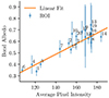 |
Fig. 2. Correlation between Bond albedo and pixel intensity on the USGS map. Each dot represents a ROI, where the mean Bond albedo and its uncertainty were derived from photometric measurements and the average pixel intensity of the corresponding region was calculated. |
Several factors could explain the modest fit quality. First, the photometric correction applied to the USGS map is empirical and may introduce artifacts, especially for images in extreme geometries or under strong non-isotropic photometry. In addition, the normalization and combination of the different filters used to create the mosaic introduce errors that are difficult to quantify. The linearity assumption of Eq. (2) could also be too simplistic. However, there is no evident higher-order relationship or alternative analytical form. Finally, the Hapke model may be an oversimplification of the true bi-directional reflectance distribution function (BRDF), especially if there are azimuthal dependences not accounted for. Despite these limitations, the root mean square (RMS) error in the Bond albedo, computed using the RMS of the differences between the ROIs’ albedos and the linear regression, is estimated to be ±0.054. This corresponds to a relative error of 9% in the Bond albedo estimate, which we consider acceptable for this study, but it should be regarded as a lower bound since additional errors inherent to the construction of the mosaic itself are not included.
4.2. Bond albedo map
We used the linear relationship in Eq. (2) to extrapolate the Bond albedo across all pixels of the USGS map, producing the high-resolution Bond albedo map of Europa shown in Fig. 3. This map, which covers nearly the entire surface of Europa (excluding the south pole data gap), will be a valuable resource for several applications. It enables calculations of the surface energy balance on a local scale and detailed thermal modeling across the entire surface without needing to invert the albedo, and it has already proven its usefulness for numerical simulations of Europa’s surface (Mergny & Schmidt 2024). This map is also beneficial for preparing quantitative observations for future missions, such as Europa Clipper and Jupiter Icy Moons Explorer (JUICE), to optimize the exposure time of the sensors.
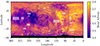 |
Fig. 3. Extrapolated Europa Bond albedo map. Anchor-point ROIs are indicated by semi-transparent white squares. The high resolution and coverage of this map will notably allow for better thermal modeling of Europa. The USGS map data gap is also present on the south pole. Longitude is expressed according to the west-increasing definition. |
Apparent discontinuities can be seen, for example around (80°W, 60°N), which are already present in the original USGS map. They reflect the limitation of the empirical photometric correction but also the nonlinearities in photometric behavior with respect to resolution. When there is a mixture of bright and dark terrains inside a pixel, the bright terrains tend to dictate the photometric behavior of the whole pixel, as shown by Pilorget et al. (2015) and Schmidt & Bourguignon (2019). This is expected, as bright terrains reflect more energy than dark ones and, hence, have more weight in the Bond albedo. A gain in resolution from future missions will resolve these apparent discontinuities. Future dedicated work on photometric merging should be carried out to improve on this aspect.
4.3. Comparison with existing data
For validation, we compared our Bond albedo map with the thermally derived values from Rathbun et al. (2010). Their study provides a Bond albedo map that covers approximately 20% of Europa’s surface, derived from the inversion of brightness temperatures measured by Galileo PPR. To allow for comparison, our map was downscaled to match the corresponding 10 ° ×10° resolution and restricted to regions where their data are available.
Figure 4 shows the differences in albedo values between the two datasets. Overall, the two methods are in general agreement: In the right panel of Fig. 4, the two approaches align closely, with Bond albedo values around 0.65. In the left panel, the two methods agree on relatively low albedo values (0.4–0.5) at low latitudes. At higher latitudes, Rathbun’s albedo values are generally higher. However, this is very consistent with Rathbun & Spencer (2020), who note that “an error in the analysis resulted in derived bolometric albedos being overestimated away from the equator”. Correcting for this would further align their values with our results.
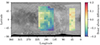 |
Fig. 4. Differences between the Bond albedo values obtained in this study and the thermally derived values from Galileo PPR (Rathbun et al. 2010). The larger differences at higher latitudes are likely due to inaccuracies in their solar flux calculations in these regions (Rathbun & Spencer 2020). |
For the 137 bins analyzed, the mean absolute difference between albedo values is ∼0.084. Discrepancies likely stem from the induced errors discussed in both methods, as well as from assumptions such as the use of a vertically homogeneous material in deriving the thermal data in Rathbun et al. (2010). Overall, while both approaches use fundamentally different methods to derive Bond albedo values, the general agreement is encouraging.
By averaging the albedo across our entire full resolution map, we obtain  , which is consistent with the globally derived Bond albedo of Europa measured from the Very Large Array (VLA) (de Pater et al. 1984),
  . This suggests that our Bond albedo values are not overestimated, as discussed in Sect. 2.1, as they are slightly lower than what has been found using other approaches in the literature.
5. Conclusion
-
We created a new Bond albedo map of Europa by combining the complete set of angular observations with a high-resolution mosaic of images. This dataset is publicly available online at DOI 10.14768/d302ffb6-ef72-4f91-a592-ff2b644aaf77 and can be used in a range of applications.
-
This albedo map will be particularly valuable for future thermal investigations of Europa. Brightness temperatures from the Europa Thermal Emission Imaging System (E-THEMIS) on board Europa Clipper will be combined with thermal models to derive the surface thermal properties. Without albedo estimates, an extra free parameter complicates the already challenging inversion process, particularly as Europa’s surface needs to be modeled as a vertically heterogeneous material (Hansen 1973; Mergny & Schmidt 2024). By providing independent albedo values, our map simplifies this process. As existing albedo estimates cover only ∼20% of Europa’s surface at a spatial resolution of ∼200 km/pixel (Rathbun et al. 2010), expanding this to nearly the entire surface at a resolution of up to ∼500 m/pixel makes our map useful for future thermal modeling of Europa.
-
The map is especially valuable for estimating the surface energy balance at high resolution. Since knowledge of the BRDF at the local scale is unavailable, it also provides a useful first-order estimate for quantitative flux estimations when planning observation sequences for missions like JUICE and Europa Clipper. For instruments like visible cameras and spectro-imagers, such albedo estimates of the observed regions provide valuable information that can be used to optimize exposure times.
-
The main limitation of this approach is due to empirical photometric correction and the linearity assumption. Several nonlinear functions can be used, but none can be justified except the photometric function itself. For instance, the nonlinearity could be due to the photometric correction when mosaicking, which in turn is due to radiative transfer nonlinearity (the nonlinear relationship between the Bond albedo and one particular angular set). This limitation would be hard to overcome in practice due to the lack of precise knowledge of the surface photometry, creating an unsolvable logical loop.
-
Future measurements from JUICE, Europa Clipper, and also JUNO will most certainly enrich the angular diversity of measurements of Jupiter’s moon and thus our knowledge of the local BRDF. Our strategy should then be revised to produce an updated Bond albedo map.
Data availability
The Bond albedo map produced in this study is available in the IPSL Data Catalog at DOI 10.14768/d302ffb6-ef72-4f91-a592-ff2b644aaf77
Acknowledgments
We acknowledge support from the “Institut National des Sciences de l’Univers” (INSU), the “Centre National de la Recherche Scientifique” (CNRS) and “Centre National d’Etudes Spatiales” (CNES) through the “Programme National de Planétologie”. We thank the anonymous reviewer and the editor for their careful reading of our manuscript and their insightful comments and suggestions. We also extend our gratitude to Dr. Julie Rathbun and Dr. John Spencer for providing the Galileo PPR albedo data used for comparison with our study.
References
- Becker, T., Archinal, B., Colvin, T., et al. 2010, Europa Voyager-Galileo SSI Global Mosaic 500m v2, US Geological Survey [Google Scholar]
- Belgacem, I., Schmidt, F., & Jonniaux, G. 2020, Icarus, 338, 113525 [NASA ADS] [CrossRef] [Google Scholar]
- Buratti, B., & Veverka, J. 1983, Icarus, 55, 93 [NASA ADS] [CrossRef] [Google Scholar]
- de Pater, I., Brown, R. A., & Dickel, J. R. 1984, Icarus, 57, 93 [NASA ADS] [CrossRef] [Google Scholar]
- Hansen, O. 1973, Icarus, 18, 237 [NASA ADS] [CrossRef] [Google Scholar]
- Hapke, B. 2012a, Theory of Reflectance and Emittance Spectroscopy, 2nd edn. (Cambridge: Cambridge University Press) [Google Scholar]
- Hapke, B. 2012b, Icarus, 221, 1079 [NASA ADS] [CrossRef] [Google Scholar]
- Mergny, C., & Schmidt, F. 2024, Planet. Sci. J., 5, 215 [NASA ADS] [CrossRef] [Google Scholar]
- Pilorget, C., Fernando, J., Ehlmann, B., & Douté, S. 2015, Icarus, 250, 188 [NASA ADS] [CrossRef] [Google Scholar]
- Rathbun, J. A., & Spencer, J. R. 2020, Icarus, 338, 113500 [NASA ADS] [CrossRef] [Google Scholar]
- Rathbun, J. A., Rodriguez, N. J., & Spencer, J. R. 2010, Icarus, 210, 763 [NASA ADS] [CrossRef] [Google Scholar]
- Schmidt, F., & Bourguignon, S. 2019, Icarus, 317, 10 [NASA ADS] [CrossRef] [Google Scholar]
- Schmidt, F., & Fernando, J. 2015, Icarus, 260, 73 [NASA ADS] [CrossRef] [Google Scholar]
- Souchon, A., Pinet, P., Chevrel, S., et al. 2011, Icarus, 215, 313 [NASA ADS] [CrossRef] [Google Scholar]
- Trumbo, S. K., Brown, M. E., & Butler, B. J. 2018, AJ, 156, 161 [NASA ADS] [CrossRef] [Google Scholar]
- van de Hulst, H. C. 1974, A&A, 35, 209 [NASA ADS] [Google Scholar]
All Figures
|
Fig. 1. 20 ROIs overlaid on the USGS map, annotated with their corresponding average Bond albedo values derived from Hapke parameter analysis. Longitude is expressed according to the west-increasing definition. |
| In the text | |
|
Fig. 2. Correlation between Bond albedo and pixel intensity on the USGS map. Each dot represents a ROI, where the mean Bond albedo and its uncertainty were derived from photometric measurements and the average pixel intensity of the corresponding region was calculated. |
| In the text | |
|
Fig. 3. Extrapolated Europa Bond albedo map. Anchor-point ROIs are indicated by semi-transparent white squares. The high resolution and coverage of this map will notably allow for better thermal modeling of Europa. The USGS map data gap is also present on the south pole. Longitude is expressed according to the west-increasing definition. |
| In the text | |
|
Fig. 4. Differences between the Bond albedo values obtained in this study and the thermally derived values from Galileo PPR (Rathbun et al. 2010). The larger differences at higher latitudes are likely due to inaccuracies in their solar flux calculations in these regions (Rathbun & Spencer 2020). |
| In the text | |
Current usage metrics show cumulative count of Article Views (full-text article views including HTML views, PDF and ePub downloads, according to the available data) and Abstracts Views on Vision4Press platform.
Data correspond to usage on the plateform after 2015. The current usage metrics is available 48-96 hours after online publication and is updated daily on week days.
Initial download of the metrics may take a while.