| Issue |
A&A
Volume 693, January 2025
|
|
|---|---|---|
| Article Number | L4 | |
| Number of page(s) | 12 | |
| Section | Letters to the Editor | |
| DOI | https://doi.org/10.1051/0004-6361/202452442 | |
| Published online | 25 December 2024 | |
Letter to the Editor
The bulk metallicity of giant planets around M stars
Department of Astrophysics, University of Zürich, Winterthurerstrasse 190, 8057 Zürich, Switzerland
⋆ Corresponding author; This email address is being protected from spambots. You need JavaScript enabled to view it.
Received:
1
October
2024
Accepted:
21
November
2024
Abstract
Determination of the bulk metallicity of giant exoplanets is essential in order to constrain their formation and evolution pathways and to compare them to the Solar System. Previous studies inferred an inverse relation between the mass and bulk metallicity. However, these studies used data mostly for planets orbiting FGK stars. The recent discoveries of giant exoplanets around M-dwarf stars present an opportunity to probe whether they follow a mass–metallicity trend that is different from that of their FGK counterparts. Using evolution models, we characterised the interiors of giant exoplanets with reliable mass–radius measurements that orbit FGK and M-dwarf stars. We then inferred the mass–metallicity trends for both populations. We find that the bulk metallicity of giant planets around M stars is overall lower than that of planets around FGK stars. This yields mass–metallicity relations for the two populations with similar slopes but significantly different offsets. The lack of metal-rich giant planets around M dwarfs could explain the difference in the inferred offset and could be a result of different formation conditions. However, there are only 20 successful bulk-metallicity retrievals for the giant planets around M dwarfs, which results in rather large uncertainties. Therefore, it is of great importance to continue detecting these planets with both transit and radial velocities. Additionally, the characterisation of the atmospheres of giant planets around M-stars would further help to constrain their interiors and facilitate investigations of the atmosphere–interior connection. Such investigations will significantly contribute to our understanding of the possible formation pathways of giant planets.
Key words: planets and satellites: composition / planets and satellites: gaseous planets / planets and satellites: interiors
© The Authors 2024
 Open Access article, published by EDP Sciences, under the terms of the Creative Commons Attribution License (https://creativecommons.org/licenses/by/4.0), which permits unrestricted use, distribution, and reproduction in any medium, provided the original work is properly cited.
This article is published in open access under the Subscribe to Open model. This email address is being protected from spambots. You need JavaScript enabled to view it. to support open access publication.
1. Introduction
The discovery and characterisation of exoplanets allows us to understand our Solar System in a wider context and to study planets in more general terms. When both the planetary mass and radius are measured, we can infer information on the mean density, and therefore the planetary bulk composition (e.g. Seager et al. 2007; Miller & Fortney 2011; Spiegel et al. 2014; Jontof-Hutter 2019). Despite the degenerate nature of the problem (e.g. Rogers & Seager 2010; Lopez & Fortney 2014), various trends have been revealed in relation to giant exoplanets. For example, we now know that the occurrence rate of giant planets increases with stellar metallicity and mass (Fischer & Valenti 2005; Johnson et al. 2010; Mortier et al. 2012, 2013; Ghezzi et al. 2018; Zhu 2019) and that there is a correlation between the mass and bulk metallicity of giant planets (Thorngren et al. 2016; Müller & Helled 2023a; Swain et al. 2024), such that smaller planetary masses are characterised by higher planetary metallicity. Furthermore, a clear correlation between stellar metallicity and the bulk metallicity of giant planets is currently not observed (Teske et al. 2019). Such trends (or the lack of them) can be used to constrain planet formation and evolution theory.
While recent decades have seen significant progress in our understanding of giant exoplanets, it must be kept in mind that most of the available data correspond to planets that orbit Sun-like stars. As a result, we still do not have a good understanding of how the observed trends and the inferred planetary properties change with stellar mass. Despite M-dwarf stars being the most common stellar type in the galaxy (Winters et al. 2015), there are currently few observed giant planets around them. While standard planet-formation theory typically predicts that giant planets are unlikely to form around such stars (Kennedy & Kenyon 2008; Schlecker et al. 2022), several planets have been observed (e.g. Hébrard et al. 2013; Bakos et al. 2015; Kanodia et al. 2023; Delamer et al. 2024). Although the sample is still rather limited, it can be compared to the population of giant planets around FGK stars. In this work, we investigate whether or not there is a difference in the bulk metallicity of giant planets that orbit FGK and M-dwarf stars.
Our paper is organised as follows. In Section 2, we describe the sample used in this work and the methods for analysing their bulk metallicities. The results of this analysis are in Section 3, where we present the inferred composition and the relations between the planetary masses, metallicities, and heavy-element masses. These results are discussed in Section 4 along with some caveats regarding our analysis. Section 5 summarises the most important conclusions from this work. Finally, more details about the exoplanetary sample, additional results, posterior distributions of the fit parameters, the influence of the age-prior choice, and an investigation of correlations are presented in the Appendix.
2. Methods
The planet sample in this work is from the updated PlanetS catalog1 (Parc et al. 2024), which uses data from the NASA Exoplanet Archive2, and was designed to provide a sample of exoplanets with reliable and robust measurements with relatively low measurement uncertainties (25% in mass and 8% in radius). Based on the mass range of planets within which objects can be considered gas giants and on the limitations of our models, our sample includes planets with masses of between 0.1 and 10 MJ. We also focus on warm giant planets with equilibrium temperatures of Teq ≲ 1000 K, corresponding to irradiation fluxes of I* < 2 × 10⁸ erg/s/cm2. These planets are not strongly inflated, and therefore characterisation of their interiors is more feasible than for hot Jupiters. We extended the sample with five recently detected giant planets around M-dwarfs: TOI-762 A b and TIC-46432937 b (Hartman et al. 2024), and TOI-6383 b, TOI-5176 A b, and TOI-6034 b (Shubham Kanodia, priv. comm.). The data were split into two sets depending on their stellar spectral types: Planets around FGK stars and planets around M-dwarf stars (with stellar effective temperatures of lower than 3900 K). In Appendix A, we show the mass–radius, mass–density, and stellar irradiation distributions for the two populations.
Using the measurements of the planetary mass (Mp), radius (R), age (τ), and irradiation (I*), the bulk heavy-element mass fraction (Z) of giant exoplanets can be inferred with thermal evolution models. Here, we used the planetsynth evolution models from Müller & Helled (2021), which are based on a grid of evolution models precalculated with the Modules for Experiments in Stellar Astrophysics code (MESA; Paxton et al. 2011, 2013, 2015, 2018, 2019; Jermyn et al. 2023) that was modified for giant planet evolution models (Müller et al. 2020a,b). These thermal evolution models are limited to a maximum planetary age of 10 Gyr, while some of the planets considered in this work are older. To address this, we implemented a new inter- and extrapolation scheme using Piecewise Cubic Hermite Interpolating Polynomials (PCHIP) from the Python package SciPy. PCHIP interpolation preserves monotonicity, which matches the physical constraint that a cooling planet’s radius decreases with time. For ages beyond 10 Gyr, the radius evolution was extrapolated. The radius of an old planet changes very slowly, and the extrapolation is expected to perform well. We validated this approach by comparing the extrapolated evolution with direct calculations with MESA and found excellent agreement: the extrapolation error was significantly below observational uncertainties.
To infer the bulk metallicity, we employed the standard Monte Carlo approach (e.g. Miller & Fortney 2011; Thorngren et al. 2016; Müller & Helled 2023b): First, a set of planetary parameters (Mi, Ri, τi) was drawn by sampling the prior distributions from observations. We assumed normal distributions for the mass and radius and a uniform distribution for the stellar age between the estimated minimum and maximum. We imposed a lower age limit of 10 Myr (due to the limitations of planetsynth), and an upper age limit corresponding to the age of the Milky Way. When no stellar age estimate was available, we assumed that the star was between 1 and 10 Gyr old. Thermal evolution models were then used to calculate the planet’s cooling in order to determine the Zi for which the radius from the model matches the observations: Rmodel(Zi | Mi, τi, I*) = Ri. We then calculated the normalised metallicity (Zi/Z*, where Z* = 0.014 ⋅ 10[Fe/H] is the stellar metallicity) and the total heavy-element mass (Mz, i = Zi ⋅ Mi). Repeating these steps yielded an estimate of the posterior distribution of Z and Mz for any given planet.
Using the No U-Turn Sampler (NUTS) Hamiltonian Monte Carlo approach (implemented in the Python package PyMC), we determined the Mp–Z/Z* and Mp–Mz relations using Bayesian linear regression on the logarithms of the variables:
 (1)
(1)
where Mp is the planet mass in MJ, y = Z/Z* or Mz in M⊕, and β0, 1 are the intercept and slope of the linear function. From the linear fit in log–log space, we also directly calculate the parameters of the corresponding power-law relationship:
 (2)
(2)
with β3 = 10β0. The uncertainties on β3 were propagated from the fit of β0. We assumed generic weakly informative priors on the fit parameters p(β0, β1)∝𝒩(μ = 0, σ = 1), where 𝒩 is the normal distribution. We considered the uncertainties in the planetary mass by assuming a generic weakly informative prior and adding a Gaussian likelihood function using the observations for the mean and standard deviation. To ensure a robust linear regression, we used the Student’s t-distribution 𝒯(μ, σ, ν) for the likelihood function of the dependent variables, where μ, σ, and ν are location, scale, and normality parameters. For μ and σ, we used the mean and standard deviation from the metallicity posteriors, which account for the uncertainty in the dependent variables. Instead of choosing a value for ν, we added an informative gamma distribution prior p(ν)∝Γ(α = 2, β = 0.1), where α and β are the shape and rate parameters. This prior is suitable as its support is between zero and infinity, and for ν → ∞, 𝒯 tends towards a Gaussian distribution 𝒯(μ, σ, ν → ∞)→𝒩(μ, σ) with mean μ and standard deviation σ.
3. Results
3.1. Planet selection
In this section, we present the metallicities inferred by the thermal evolution models and the fits for the Mp–Z/Z* and Mp–Mz relations for warm giant planets as described in Section 2. These relations were derived for two mass ranges: the full sample with 0.1 ≤ Mp(MJ)≤10, and a mass-limited sample with 0.3 ≤ Mp(MJ)≤2. The full sample includes as many planets as possible within the limitations of our models, which should yield lower uncertainties of the fit parameters. However, analyses of the mass–radius relationships (Chen & Kipping 2017; Bashi et al. 2017; Edmondson et al. 2023; Müller et al. 2024; Parc et al. 2024) and planet-formation considerations (Helled 2023) suggest that giant planets may be better described as the population with masses beyond about 0.3 MJ. For the upper mass limit in this second sample, we chose 2 MJ. This limit is based on the masses of the current observed giant planets around M-dwarf stars and considerations of their formation pathways (Helled et al. 2014). We consider this mass-limited sample to better represent the class of giant planets and therefore use it here to derive the Mp–Z/Z* and Mp–Mz relations. The results for the full sample are presented in Appendix B. The planets and their inferred bulk metallicites and heavy-element masses are listed in Table A.1.
3.2. Mass-limited sample
We obtained 49 and 15 successful metallicity retrievals for planets around FGK and M-dwarf stars in the preferred mass-limited sample. The Bayesian regression resulted in the following power-law relation for Mp–Z/Z*:
 (3)
(3)
where Mp is in Jupiter masses. The resulting fits for the Mp–Mz relation are given by:
 (4)
(4)
where Mz is in Earth units. All fit parameters are tabulated in Appendix C in Tables C.1 and C.2, and their posterior distributions from the Bayesian inference are shown in Figures C.1 and C.2.
Figure 1 shows the inferred normalised metallicities, heavy-element masses, and the two fits. Both populations of planets show a decreasing trend for the normalised metallicity and an increasing trend for the heavy-element mass. There is a considerable offset between the fits for the planets around FGK and M-dwarf stars. While the scatter is fairly large, we find that giant planets around M dwarfs are overall metal-poor compared to their FGK counterparts.
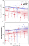 |
Fig. 1. Normalised metallicity (top) and heavy-element mass (bottom) as a function of planet mass for 0.3 ≤ Mp(MJ)≤2. The scatter points and error bars show the normalised metallicity or heavy element mass inferred by the thermal evolution models. Solid lines show the fits constructed by Bayesian regression, and the shaded contours are the 1σ and 2σ uncertainties. Planets around FGK stars are depicted in blue, while those around M-dwarfs are in red. The grey dashed line shows the fit from Thorngren et al. (2016) for comparison. |
We compare our results to those presented in Thorngren et al. (2016). The results deviate for the two populations. Our results are quite similar to those of Thorngren et al. (2016) with regard to planets around FGK stars, but our results suggest a lower metal enrichment. Moreover, we find numerous planets with normalised metallicities of about one or less, that is, planets with bulk metallicities that are stellar or even substellar. Similarly, we also find planets that contain less than 10 M⊕ of heavy elements, a value that traditionally corresponded to the critical core mass to initiate rapid gas accretion (e.g. Helled et al. 2014; D’Angelo & Lissauer 2018). However, today, we know that the critical core mass can vary and depends on the exact formation conditions (e.g. Ikoma et al. 2001; Movshovitz et al. 2010; Venturini et al. 2015). We suggest that formation models should be used to carry out a detailed investigation into whether or not gas accretion is indeed initiated at smaller core mass for giant planets forming around M-dwarf stars.
Besides the different data used, the most likely factor responsible for the lower metal enrichment that we see compared to the findings of Thorngren et al. is the hydrogen–helium equation of state: we used the Chabrier et al. (2019) equation of state, while Thorngren et al. used SCvH (Saumon et al. 1995). It was shown that using the Chabrier et al. equation of state leads to smaller planets due to hydrogen being denser under certain pressure–temperature conditions, leading to lower inferred metallicities (Müller et al. 2020a; Howard & Guillot 2023; Sur et al. 2024; Howard et al. 2025). In particular, Müller et al. (2020a) identified several planets that appear to be inflated, although their irradiation is insufficiently strong to explain their observed sizes.
The downside of the mass-limited sample is its reduced size, and the uncertainty of the fits therefore increases. However, as shown in Figures C.1 and C.2, the y-intercepts for the two populations are incompatible within more than two σ. Despite the large uncertainties, we suggest that, for the available data, the result that giant planets around M-dwarf planets are metal poor is robust.
3.3. Correlations with the stellar metallicity
In this section, we test whether our predictions for the planetary bulk metallicity and heavy-element mass are correlated with stellar metallicity. Additional correlations with other stellar and planetary parameters are investigated in Appendix E. As in the previous analysis, we split the data into planets around FGK and M-dwarf stars and used two different mass ranges. For each pairing, we calculated Kendall’s tau rank correlation coefficient and its associated p-value to determine whether or not the correlation is statistically significant.
For the heavy-element mass, we used the residuals to investigate the correlation. The residual heavy-element mass of a planet was calculated with its inferred heavy-element mass divided by the value predicted using Eq. (4) or (B.2) depending on whether the full or mass-limited data were used. The residual represents the deviation from the value expected from the planetary mass alone. Therefore, there is an advantage to using the residual in that it highlights whether or not the deviation from the fit correlates with the stellar metallicity.
The bulk metallicity and residual heavy-element mass as functions of stellar metallicity are shown in Figure 2. For FGK stars, we find that the planetary bulk metallicity is correlated with the stellar metallicity in the full sample (τ = 0.14, p = 0.03) and the mass-limited sample (τ = 0.27, p = 0.008). Similarly, the stellar metallicity is also correlated with the residual heavy-element mass in both the full (τ = 0.25, p = 0.002) and the mass-limited sample (τ = 0.26, p = 0.008). We do not find any statistically significant correlation for the planets around M-dwarf stars. This is probably due to the limited number of detected planets.
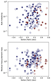 |
Fig. 2. Planetary bulk metallicity (top) and residual heavy-element mass (bottom) vs. stellar metallicity. Planets around FGK and M-dwarf stars are depicted in blue circles and red hexagons. Filled symbols mark planets that were included in the mass-limited sample. For FGK stars, the bulk metallicity and residual heavy-element mass are moderately correlated with stellar metallicity. |
The inferred correlation between the stellar metallicity and the residual heavy-element mass is at odds with the findings of previous analyses (Thorngren et al. 2016; Teske et al. 2019). In particular, Teske et al. (2019) did not find a clear correlation between those two values, although such a correlation is predicted from formation models (e.g. Mordasini 2014). The discrepancy is likely due to the significantly higher number of planets in our data. Our analysis includes up to 104 planets, while Teske et al. (2019) was limited to 24 planets. We also note that the lack of correlation for M dwarfs may be due to the limited data available. While outside the scope of this work, a thorough analysis of potential correlations between the composition of stars and their planets is desirable.
4. Discussion
The results presented here provide new insights into our understanding of giant planets across stellar masses. However, this is only the first step. Below, we briefly describe the limitations in terms of the data and the modelling approach, and discuss our results in the wider context of giant planet formation theory.
First, it should be noted that this study used a relatively low number of observed giant planets around M dwarfs, due in part to the low occurrence rate of giant planets around M dwarfs (Endl et al. 2006; Johnson et al. 2010; Maldonado et al. 2019; Schlecker et al. 2022; Gan et al. 2023; Bryant et al. 2023). This leads to rather large uncertainties in the fit parameters (see Section 3.2 and Appendix B). Despite this, irrespective of the imposed mass limits, the fits to the two populations are inconsistent within at least about 2σ. There could be an observational bias towards larger, metal-poor giant planets, which are more readily detected. However, objects with smaller masses and radii or larger masses and similar radii are being observed. They may, however, be rare and underrepresented in the current sample. Alternatively, due to the limited number of planets in the M-dwarf sample, it is possible that a greater number of metal-poor giant planets were observed by chance. Therefore, it is desirable to have a large data sample and we encourage observers to detect more giant planets around M dwarfs with both transit and radial velocity methods.
Second, the evolution models used to infer the planetary composition are based on several assumptions and include uncertainties that could affect the results. The largest effects are linked to the equation of state, the assumed chemical composition of the heavy elements, the interior temperature and composition profiles, and the atmospheric model (Thorngren et al. 2016; Poser et al. 2019; Müller et al. 2020a; Poser & Redmer 2024). However, these model uncertainties should apply to planets around FGK and M-dwarf stars equally. The two populations are fairly similar concerning their incident stellar irradiation (Figure A.2). As a result, differences in their atmospheres are unlikely to be caused by the heat they receive from their stars. While the absolute values of the inferred bulk metallicities would be affected by changing the model details and the inferred composition could be shifted, the difference between the populations should remain.
Third, a key challenge regarding the characterisation of giant planets around M-dwarfs is that the stellar ages are typically poorly constrained. When an age estimate was unavailable, we used an uninformative prior from 1 to 10 Gyr. Given that many of the M dwarfs in the sample are likely older than a few gigayears, our generous choice biases our results towards higher metallicities. This is because, for a given radius, a younger planetary age increases the inferred metallicity (compared to older ages). As a result, our conclusion that the metallicities of giant planets around M-stars are lower than those of giant planets orbiting Sun-like stars is robust. Further details can be found in Appendix D, where we repeat our analysis assuming different age ranges.
Finally, it is interesting to speculate on how our results can be used to constrain giant planet formation around M dwarfs. In the core accretion scenario (e.g. Pollack et al. 1996), the formation of a giant planet around a low-mass star takes longer mainly due to the longer orbital timescales (for a given location) and lower protoplanetary disc masses (Andrews et al. 2013; Pascucci et al. 2016). Core-accretion planet formation models generally fail to produce giant planets within reasonable disc lifetimes (Laughlin et al. 2004; Burn et al. 2021; Schlecker et al. 2022). An alternative formation pathway would be gravitational (disc) instability, in which the giant planet is formed during the proto-stellar phase of massive, gravitationally unstable protoplanetary discs (e.g. Boss 1997, 2006; Boss & Kanodia 2023).
The slopes of the mass–metallicity and M–Mz trends we infer here appear similar for both planet populations. These inverse relations were previously suggested to be compatible with planets that formed by core accretion (Miller & Fortney 2011; Thorngren et al. 2016). Indeed, in the core-accretion framework, the lower heavy-element content of giant planets around M dwarfs could be seen as a result of long formation timescales or the reduced availability of solids. Interestingly, the slow growth of the M-dwarf giant planets is expected to lead to highly extended composition gradients and non-adiabatic cooling for a large portion of the interior (e.g., Helled & Stevenson 2017; Vazan & Helled 2020). In that case, the planetary interiors could be hotter than our homogeneous evolution models predict, which would cause us to underestimate the bulk metallicity (for a given radius, a hotter planet can contain more heavy elements).
At the same time, lower metallicities can also be the result of formation by disc instability if fewer heavy elements are accreted post-formation due to different disc properties and formation location (e.g. Helled & Schubert 2009). At present, given the limited data and uncertainties in theoretical models, it is not possible to discriminate between these two formation paths. It is clear that further theoretical investigation of the expected metallicities of giant planets in both formation models is required.
5. Conclusions
We investigated the correlation between the bulk metallicity and planetary mass of giant planets around M-stars. The exoplanetary data we used are mostly from the updated PlanetS catalogue but we complemented these with recently confirmed observations of giant planets around M-dwarf stars. The sample resulted in 104 successful bulk-metallicity retrievals for FGK and 20 for M-dwarf stars. We performed Bayesian regression with these results to derive updated M–Z/Z* and M–Mz relations. Our main results can be summarised as follows:
-
The currently available data suggest that there is a lack of metal-rich giant planets around M dwarfs compared to their FGK-stars counterparts.
-
The M–Z/Z* and M–Mz relations depend on the planetary mass range used for the fit.
-
For masses of between 0.1 and 10 MJ, we find the slopes and magnitudes of the metallicity and heavy-element mass fits are inconsistent between the two populations.
-
For masses between 0.3 and 1.0, the slopes are fairly similar, but there is still a significant offset that predicts a lower bulk metallicity for giant planets around M dwarfs.
-
For giant planets around FGK stars, we find that the planetary bulk metallicity and residual heavy-element mass are moderately correlated with the stellar metallicity.
Currently, the number of giant planets with measured mass and radius around M dwarfs is still limited. Future measurements of planets with masses of between approximately 0.3 and 2 MJ around M dwarfs will help to identify the difference between the two populations. Also, measurements of the atmospheric composition of giant planets around M dwarfs will facilitate the direct comparison of the atmospheric composition of planets around FGK and M-dwarf stars, and reveal the relationship between planetary mass and atmospheric metallicity (Welbanks et al. 2019; Edwards et al. 2023; Sun et al. 2024; Kanodia et al. 2024). Knowledge of the atmospheric composition, together with measured masses and radii, will also improve the interior characterisation. This will provide a unique opportunity to study the atmosphere–interior connection of giant planets across different stellar masses and to improve our understanding of giant planet formation in general.
Data availability
Full Table A.1 is available at the CDS via anonymous ftp to cdsarc.cds.unistra.fr (130.79.128.5) or via https://cdsarc.cds.unistra.fr/viz-bin/cat/J/A+A/693/L4
Acknowledgments
We thank Shubham Kanodia for sharing data and fruitful discussions, and the anonymous reviewer for providing useful comments. We acknowledge support from the Swiss National Science Foundation (SNSF) grant 200020_215634 and the National Centre for Competence in Research ‘PlanetS’ supported by SNSF. This research used data from the NASA Exoplanet Archive, which is operated by the California Institute of Technology, under contract with the National Aeronautics and Space Administration under the Exoplanet Exploration Program. Extensive use was also made of the Python packages Jupyter (Kluyver et al. 2016), Matplotlib (Hunter 2007), NumPy (Harris et al. 2020), pandas (Wes McKinney 2010), planetsynth (Müller & Helled 2021), PyMC (Oriol et al. 2023), and SciPy (Virtanen et al. 2020).
References
- Andrews, S. M., Rosenfeld, K. A., Kraus, A. L., & Wilner, D. J. 2013, ApJ, 771, 129 [Google Scholar]
- Bakos, G. Á., Hartman, J. D., Bhatti, W., et al. 2015, AJ, 149, 149 [Google Scholar]
- Bashi, D., Helled, R., Zucker, S., & Mordasini, C. 2017, A&A, 604, A83 [NASA ADS] [CrossRef] [EDP Sciences] [Google Scholar]
- Boss, A. P. 1997, Science, 276, 1836 [Google Scholar]
- Boss, A. P. 2006, ApJ, 643, 501 [Google Scholar]
- Boss, A. P., & Kanodia, S. 2023, ApJ, 956, 4 [NASA ADS] [CrossRef] [Google Scholar]
- Bryant, E. M., Bayliss, D., & Van Eylen, V. 2023, MNRAS, 521, 3663 [CrossRef] [Google Scholar]
- Burn, R., Schlecker, M., Mordasini, C., et al. 2021, A&A, 656, A72 [NASA ADS] [CrossRef] [EDP Sciences] [Google Scholar]
- Chabrier, G., Mazevet, S., & Soubiran, F. 2019, ApJ, 872, 51 [NASA ADS] [CrossRef] [Google Scholar]
- Chen, J., & Kipping, D. 2017, ApJ, 834, 17 [Google Scholar]
- D’Angelo, G., & Lissauer, J. J. 2018, in Handbook of Exoplanets, eds. H. J. Deeg, & J. A. Belmonte, 140 [Google Scholar]
- Delamer, M., Kanodia, S., Cañas, C. I., et al. 2024, ApJ, 962, L22 [NASA ADS] [CrossRef] [Google Scholar]
- Edmondson, K., Norris, J., & Kerins, E. 2023, arXiv e-prints [arXiv:2310.16733] [Google Scholar]
- Edwards, B., Changeat, Q., Tsiaras, A., et al. 2023, ApJS, 269, 31 [NASA ADS] [CrossRef] [Google Scholar]
- Endl, M., Cochran, W. D., Kürster, M., et al. 2006, ApJ, 649, 436 [Google Scholar]
- Fischer, D. A., & Valenti, J. 2005, ApJ, 622, 1102 [NASA ADS] [CrossRef] [Google Scholar]
- Gan, T., Wang, S. X., Wang, S., et al. 2023, AJ, 165, 17 [NASA ADS] [CrossRef] [Google Scholar]
- Ghezzi, L., Montet, B. T., & Johnson, J. A. 2018, ApJ, 860, 109 [Google Scholar]
- Harris, C. R., Millman, K. J., van der Walt, S. J., et al. 2020, Nature, 585, 357 [NASA ADS] [CrossRef] [Google Scholar]
- Hartman, J. D., Bayliss, D., Brahm, R., et al. 2024, AJ, 168, 202 [Google Scholar]
- Hébrard, G., Collier Cameron, A., Brown, D. J. A., et al. 2013, A&A, 549, A134 [NASA ADS] [CrossRef] [EDP Sciences] [Google Scholar]
- Helled, R. 2023, A&A, 675, L8 [NASA ADS] [CrossRef] [EDP Sciences] [Google Scholar]
- Helled, R., & Schubert, G. 2009, ApJ, 697, 1256 [NASA ADS] [CrossRef] [Google Scholar]
- Helled, R., & Stevenson, D. 2017, ApJ, 840, L4 [NASA ADS] [CrossRef] [Google Scholar]
- Helled, R., Bodenheimer, P., Podolak, M., et al. 2014, in Protostars and Planets VI, eds. H. Beuther, R. S. Klessen, C. P. Dullemond, & T. Henning, 643 [Google Scholar]
- Howard, S., & Guillot, T. 2023, A&A, 672, L1 [NASA ADS] [CrossRef] [EDP Sciences] [Google Scholar]
- Howard, S., Helled, R., & Müller, S. 2025, A&A, in press, https://doi.org/10.1051/0004-6361/202452783 [Google Scholar]
- Hunter, J. D. 2007, Comput. Sci. Eng., 9, 90 [NASA ADS] [CrossRef] [Google Scholar]
- Ikoma, M., Emori, H., & Nakazawa, K. 2001, ApJ, 553, 999 [NASA ADS] [CrossRef] [Google Scholar]
- Jermyn, A. S., Bauer, E. B., Schwab, J., et al. 2023, ApJS, 265, 15 [NASA ADS] [CrossRef] [Google Scholar]
- Johnson, J. A., Aller, K. M., Howard, A. W., & Crepp, J. R. 2010, PASP, 122, 905 [Google Scholar]
- Jontof-Hutter, D. 2019, Ann. Rev. Earth Planet. Sci., 47, 141 [Google Scholar]
- Kanodia, S., Mahadevan, S., Libby-Roberts, J., et al. 2023, AJ, 165, 120 [NASA ADS] [CrossRef] [Google Scholar]
- Kanodia, S., Cañas, C. I., Mahadevan, S., et al. 2024, AJ, 167, 161 [Google Scholar]
- Kennedy, G. M., & Kenyon, S. J. 2008, ApJ, 673, 502 [Google Scholar]
- Kluyver, T., Ragan-Kelley, B., Pérez, F., et al. 2016, in Positioning and Power in Academic Publishing: Players, Agents and Agendas, eds. F. Loizides, & B. Scmidt (Netherlands: IOS Press), 87 [Google Scholar]
- Laughlin, G., Bodenheimer, P., & Adams, F. C. 2004, ApJ, 612, L73 [NASA ADS] [CrossRef] [Google Scholar]
- Lopez, E. D., & Fortney, J. J. 2014, ApJ, 792, 1 [Google Scholar]
- Maldonado, J., Villaver, E., Eiroa, C., & Micela, G. 2019, A&A, 624, A94 [NASA ADS] [CrossRef] [EDP Sciences] [Google Scholar]
- Miller, N., & Fortney, J. J. 2011, ApJ, 736, L29 [NASA ADS] [CrossRef] [Google Scholar]
- Mordasini, C. 2014, A&A, 572, A118 [NASA ADS] [CrossRef] [EDP Sciences] [Google Scholar]
- Mortier, A., Santos, N. C., Sozzetti, A., et al. 2012, A&A, 543, A45 [NASA ADS] [CrossRef] [EDP Sciences] [Google Scholar]
- Mortier, A., Santos, N. C., Sousa, S., et al. 2013, A&A, 551, A112 [NASA ADS] [CrossRef] [EDP Sciences] [Google Scholar]
- Movshovitz, N., Bodenheimer, P., Podolak, M., & Lissauer, J. J. 2010, Icarus, 209, 616 [Google Scholar]
- Müller, S., & Helled, R. 2021, MNRAS, 507, 2094 [CrossRef] [Google Scholar]
- Müller, S., & Helled, R. 2023a, A&A, 669, A24 [NASA ADS] [CrossRef] [EDP Sciences] [Google Scholar]
- Müller, S., & Helled, R. 2023b, Front. Astron. Space Sci., 10, 1179000 [CrossRef] [Google Scholar]
- Müller, S., Ben-Yami, M., & Helled, R. 2020a, ApJ, 903, 147 [Google Scholar]
- Müller, S., Helled, R., & Cumming, A. 2020b, A&A, 638, A121 [Google Scholar]
- Müller, S., Baron, J., Helled, R., Bouchy, F., & Parc, L. 2024, A&A, 686, A296 [NASA ADS] [CrossRef] [EDP Sciences] [Google Scholar]
- Oriol, A.-P., Virgile, A., Colin, C., et al. 2023, PeerJ Comput. Sci., 9, e1516 [CrossRef] [Google Scholar]
- Parc, L., Bouchy, F., Venturini, J., Dorn, C., & Helled, R. 2024, A&A, 688, A59 [NASA ADS] [CrossRef] [EDP Sciences] [Google Scholar]
- Pascucci, I., Testi, L., Herczeg, G. J., et al. 2016, ApJ, 831, 125 [Google Scholar]
- Paxton, B., Bildsten, L., Dotter, A., et al. 2011, ApJS, 192, 3 [Google Scholar]
- Paxton, B., Cantiello, M., Arras, P., et al. 2013, ApJS, 208, 4 [Google Scholar]
- Paxton, B., Marchant, P., Schwab, J., et al. 2015, ApJS, 220, 15 [Google Scholar]
- Paxton, B., Schwab, J., Bauer, E. B., et al. 2018, ApJS, 234, 34 [NASA ADS] [CrossRef] [Google Scholar]
- Paxton, B., Smolec, R., Schwab, J., et al. 2019, ApJS, 243, 10 [Google Scholar]
- Pollack, J. B., Hubickyj, O., Bodenheimer, P., et al. 1996, Icarus, 124, 62 [NASA ADS] [CrossRef] [Google Scholar]
- Poser, A. J., & Redmer, R. 2024, MNRAS, 529, 2242 [NASA ADS] [CrossRef] [Google Scholar]
- Poser, A. J., Nettelmann, N., & Redmer, R. 2019, Atmosphere, 10, 664 [NASA ADS] [CrossRef] [Google Scholar]
- Rogers, L. A., & Seager, S. 2010, ApJ, 716, 1208 [NASA ADS] [CrossRef] [Google Scholar]
- Saumon, D., Chabrier, G., & van Horn, H. M. 1995, ApJS, 99, 713 [NASA ADS] [CrossRef] [Google Scholar]
- Schlecker, M., Burn, R., Sabotta, S., et al. 2022, A&A, 664, A180 [NASA ADS] [CrossRef] [EDP Sciences] [Google Scholar]
- Seager, S., Kuchner, M., Hier-Majumder, C. A., & Militzer, B. 2007, ApJ, 669, 1279 [NASA ADS] [CrossRef] [Google Scholar]
- Spiegel, D. S., Fortney, J. J., & Sotin, C. 2014, Proc. Natl. Acad. Sci., 111, 12622 [NASA ADS] [CrossRef] [Google Scholar]
- Sun, Q., Wang, S. X., Welbanks, L., Teske, J., & Buchner, J. 2024, AJ, 167, 167 [CrossRef] [Google Scholar]
- Sur, A., Su, Y., Tejada Arevalo, R., Chen, Y.-X., & Burrows, A. 2024, ApJ, 971, 104 [Google Scholar]
- Swain, M. R., Hasegawa, Y., Thorngren, D. P., & Roudier, G. M. 2024, Space Sci. Rev., 220, 61 [Google Scholar]
- Teske, J. K., Thorngren, D., Fortney, J. J., Hinkel, N., & Brewer, J. M. 2019, AJ, 158, 239 [NASA ADS] [CrossRef] [Google Scholar]
- Thorngren, D. P., Fortney, J. J., Murray-Clay, R. A., & Lopez, E. D. 2016, ApJ, 831, 64 [NASA ADS] [CrossRef] [Google Scholar]
- Vazan, A., & Helled, R. 2020, A&A, 633, A50 [NASA ADS] [CrossRef] [EDP Sciences] [Google Scholar]
- Venturini, J., Alibert, Y., Benz, W., & Ikoma, M. 2015, A&A, 576, A114 [NASA ADS] [CrossRef] [EDP Sciences] [Google Scholar]
- Virtanen, P., Gommers, R., Oliphant, T. E., et al. 2020, Nat. Methods, 17, 261 [Google Scholar]
- Welbanks, L., Madhusudhan, N., Allard, N. F., et al. 2019, ApJ, 887, L20 [NASA ADS] [CrossRef] [Google Scholar]
- Wes McKinney 2010, in Proceedings of the 9th Python in Science Conference, eds. S. van der Walt, & J. Millman, 56 [CrossRef] [Google Scholar]
- Winters, J. G., Henry, T. J., Lurie, J. C., et al. 2015, AJ, 149, 5 [Google Scholar]
- Zhu, W. 2019, ApJ, 873, 8 [NASA ADS] [CrossRef] [Google Scholar]
Appendix A: Exoplanetary sample
Figure A.1 shows the warm giant planet sample in the mass-radius and mass-density space. The full dataset included 110 and 20 planets around FGK and M-dwarf stars, respectively. There is no immediately obvious difference between the two populations evident. This highlights the need for thermal evolution models to characterise warm giant planets. The planets in the sample, their inferred heavy-element masses and normalised metallicities are listed in Table A.1.
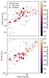 |
Fig. A.1. Mass-radius (top) and mass-density relations (bottom) for giant planets around FGK stars (circles) and M-dwarfs (hexagons). The colours indicate the equilibrium temperature. |
Planets in the sample and some of their properties.
In the sample, there were 11 low-mass planets around FGK stars (< 0.9 MJ) with very high densities (> 1.1 g/cm3). Here, we briefly discuss whether they could explain the differences in the mass-metallicity trend that we observed. Four planets were too dense for a successful interior characterisation with our models and were not included in the analysis. To explain the observations, these planets would need to consist of large fractions of rocks or iron. For the other seven planets, three were excluded from our preferred sample due to being less massive than 0.3 MJ. The remaining four planets were used in the fitting procedure. Two were found to be quite metal-rich (Z/Z* ≃ 30 − 40), and two were moderately metal-rich (Z/Z* ≃ 10 − 15). Given the large number of giant planets around FGK stars in our dataset, we don’t expect the two metal-rich planets with anomalously high densities to significantly influence the inferred M-Mz and M-Z/Z* relations.
Figure A.2 shows the distribution of the stellar irradiation for the two populations. The distributions are similar, but the peak for the planets around FGK stars is around I* = 108 compared to around 5 × 10⁷ erg/s/cm2 for M dwarfs. Therefore, the former have higher equilibrium temperatures than the latter. Since M-dwarf stars are colder, this also means that the planets around them have very short orbital periods.
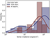 |
Fig. A.2. Histograms and kernel density estimates of the stellar irradiation for the giant planets around FGK stars (blue) and M dwarfs (red). |
Appendix B: Mp-Z/Z* and Mp-Mz relations for the full sample
In the full sample (0.1 ≤ Mp(MJ)≤10), there were 103 successful bulk-metallicity retrievals for FGK stars and 20 for M-dwarf stars. The reasons for an unsuccessful retrieval are that the planet’s density is too high or low at its suggested age. The inferred mass-metallicity relations were
 (B.1)
(B.1)
For the heavy-element masses, the relations were
 (B.2)
(B.2)
Figure B.1 shows the inferred normalised metallicities, heavy-element masses, and the two fits. As before, the fit parameters are tabulated and their posterior distributions are shown in Appendix C.
where Mz is in Earth units.
Compared to the results in Section 3.2, the larger mass range yielded significantly different Mp-Z/Z* and Mp-Mz relations. We find a qualitatively similar inverse trend between the masses and bulk metallicities. However, for both populations, the slopes are significantly steeper and do not agree with the results from Thorngren et al. (2016). As already discussed in Section 3.2, we generally infer a lower metallicity than Thorngren et al., mainly due to the more realistic hydrogen-helium equation of state used in our models. The Mp-Z/Z* relation also declines more rapidly for the giant planets around M dwarfs and predicts a lower enrichment for all masses for these planets. The main conclusion is consistent with our previous analysis: i.e., giant planets around M dwarfs are less metal-rich. This is particularly true for the planets more massive than about a Saturn mass.
For the Mp-Mz relations, there are larger differences compared to the mass-limited sample and the trends show different behaviours for the two populations: The heavy-element mass increases with mass for the giant planets around FGK stars, and decreases for those around M dwarfs. As for the mass-metallicity trend, our inferred slopes disagree with the results from Thorngren et al. (2016). However, the uncertainty on the slope in the latter case is large, and a flat or positive slope is consistent within two σ.
Looking closer at the inferred composition reveals a potential issue with the fit for the planets around M dwarfs. The low-mass planets are metal-rich, while those above about a Saturn mass are generally metal-poor. Therefore, to fit the low- and high-mass planets the slope becomes very steep, resulting in a negative Mp-Mz trend. As discussed previously (see Section 3.2), giant planes may better be classified as having masses beyond about 0.3MJ. We therefore suggest that the results presented in Section 3.2 for the mass-limited sample are more realistic and should be preferred.
Appendix C: Fit parameters and posterior distributions
Tables C.1 and C.2 list the parameters for the Mp-Z/Z* and Mp-Mz relations, and Figures C.1 and C.2 show the posterior distributions of the inferred intercept (β0) and slopes (β1). The fit parameters are defined in Equations 1 and 2 and are listed for the two different mass ranges.
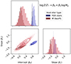 |
Fig. C.1. Posterior distributions of the inferred intercept (β0) and slope (β1) for the Mp-Z/Z* relation. The results are coloured depending on the host-star type (blue for FGK stars and red for M dwarfs). The lighter-shaded results are for the fit for the mass-limited sample 0.3 ≤ Mp(MJ)≤2. |
Fit parameters for the mass-metallicity relations.
Same as Table C.1, but for the relations between the planetary mass Mp(MJ) and the heavy-element mass Mz(M⊕)
These results demonstrate that for both the relations the β0-β1 posteriors are distinct. They depend on the host-star type as well as the mass range of the sample. For the full mass range (0.1 ≤ Mp(MJ)≤10), the slopes are incompatible for the two populations. For the smaller mass range (0.3 ≤ Mp(MJ)≤2), the slopes for the planets around M-dwarf stars are compatible with those around FGK stars. However, they have a large uncertainty. In all the cases, the intercepts (β0) are inconsistent for the two populations within more than two σ. We therefore concluded that planets around M-dwarfs are metal-poor compared to those around FGK stars.
Appendix D: Influence of the uniform age priors for unknown M dwarf ages
As stated in Section 2, whenever a stellar age estimate was unavailable, we used a uniform prior from 1 to 10 Gyr. This was the case for 8 out of 20 M dwarfs. Here, we investigate how this influences our results. To isolate the effect of the age priors, we focused on the heavy-element mass since its determination does not rely on stellar metallicity measurements. For both the full and mass-limited samples we re-inferred the heavy-element masses of the M-dwarf planets twice more. Once with a young age uniform prior of 1 to 3 Gyr, and once with an old age prior of 7 to 10 Gyr.
The resulting data and linear fits are shown in Figure D.1. Younger age priors lead to higher inferred heavy-element for planets with unknown ages. This shifts the M-Mz relation more towards that of the FGK stars. If the eight planets with unknown ages were indeed all very young (1 to 3 Gyr), it would decrease the likelihood that the two planet populations are different concerning their heavy-element masses. Previously, the M-Mz relations were inconsistent to within about two σ, and as Figure D.1 shows this would be reduced to about one σ for the young-age prior. The overall Mp-Z/Z* and Mp-Mz trends are also consistent with what was presented in Section 3.2 and Appendix B. We note, however, that it is very unlikely that all of these planets are this young, and therefore our nominal results are more likely.
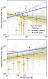 |
Fig. D.1. Heavy-element mass as a function of planet mass for the full (0.1 ≤ Mp(MJ)≤10, top) and limited samples (0.3 ≤ Mp(MJ)≤2, bottom). The scatter points and error bars show the inferred heavy-element mass by the thermal evolution models. Solid lines show the fits constructed by Bayesian regression, and the shaded contours are the one and two σ uncertainties. Planets around FGK stars are depicted in blue, while planets around M-dwarfs are orange and green depending on the age prior that was used (see text for details). |
Appendix E: Correlations with planetary and stellar properties
In this section, we test whether our predictions for the residual normalised metallicity and heavy-element mass are correlated with the stellar age, stellar mass, planetary instellation flux, orbital period, semi-major axis and eccentricity. Similar to our previous analyses, we split the data into planets around FGK and M-dwarf stars and the full and limited mass ranges (see Section 3.1). To ensure that we are testing for correlations not accounted for in our fits, we used the residuals, which are the ratios of the calculated values and the ones predicted from the best fits (see 3.3. Similar to the results presented in Section 3.3, we calculated Kendall’s tau rank correlation coefficient and its associated p-value for each pairing.
For giant planets around M-dwarf stars we did not find any statistically significant correlations. For giant planets around FGK stars with 0.1 ≤ M ≤ 10MJ, however, the residual normalised metallicity was found to be slightly correlated with the stellar mass (τ = 0.14, p = 0.05), the orbital period (τ = 0.16, p = 0.02), the semi-major axis (τ = 0.16, p = 0.02), and the eccentricity (τ = 0.15, p = 0.03). For the mass-limited sample, there was also a negative correlation with the instellation flux (τ = −0.23, p = 0.02).
For the full mass range, the residual heavy-element mass was similarly correlated with the stellar mass (τ = 0.14, p = 0.03), the orbital period (τ = 0.15, p = 0.03), the semi-major axis (τ = 0.15, p = 0.03) and the eccentricity (τ = 0.21, p = 0.002). For this sample, we also obtained a negative correlation with the stellar age (τ = −0.21, p = 0.04), and a similar correlation with the instellation flux for the mass-limited sample (τ = −0.20, p = 0.03).
Overall, these inferred correlations are generally weak with relatively large p-values for the FGK sample. The lack of correlations for the planets around M-dwarf stars is probably caused by the limited data. Future research could re-visit this topic once more data are available.
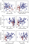 |
Fig. E.1. The residual normalised metallicity (the ratio of the calculated and predicted values) against various planetary and stellar properties. Planets around FGK and M-dwarf stars are depicted in blue circles and red hexagons. Filled symbols mark planets in the mass-limited sample (see text for further details). |
 |
Fig. E.2. The residual heavy-element mass (the ratio of the calculated and predicted values) against various planetary and stellar properties. Planets around FGK and M-dwarf stars are depicted in blue circles and red hexagons. Filled symbols mark planets in the mass-limited sample. See text for details. |
All Tables
Same as Table C.1, but for the relations between the planetary mass Mp(MJ) and the heavy-element mass Mz(M⊕)
All Figures
|
Fig. 1. Normalised metallicity (top) and heavy-element mass (bottom) as a function of planet mass for 0.3 ≤ Mp(MJ)≤2. The scatter points and error bars show the normalised metallicity or heavy element mass inferred by the thermal evolution models. Solid lines show the fits constructed by Bayesian regression, and the shaded contours are the 1σ and 2σ uncertainties. Planets around FGK stars are depicted in blue, while those around M-dwarfs are in red. The grey dashed line shows the fit from Thorngren et al. (2016) for comparison. |
| In the text | |
|
Fig. 2. Planetary bulk metallicity (top) and residual heavy-element mass (bottom) vs. stellar metallicity. Planets around FGK and M-dwarf stars are depicted in blue circles and red hexagons. Filled symbols mark planets that were included in the mass-limited sample. For FGK stars, the bulk metallicity and residual heavy-element mass are moderately correlated with stellar metallicity. |
| In the text | |
|
Fig. A.1. Mass-radius (top) and mass-density relations (bottom) for giant planets around FGK stars (circles) and M-dwarfs (hexagons). The colours indicate the equilibrium temperature. |
| In the text | |
|
Fig. A.2. Histograms and kernel density estimates of the stellar irradiation for the giant planets around FGK stars (blue) and M dwarfs (red). |
| In the text | |
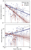 |
Fig. B.1. Same as Figure 1, but the fits were for the full planet sample with 0.1 ≤ Mp(MJ)≤10. |
| In the text | |
|
Fig. C.1. Posterior distributions of the inferred intercept (β0) and slope (β1) for the Mp-Z/Z* relation. The results are coloured depending on the host-star type (blue for FGK stars and red for M dwarfs). The lighter-shaded results are for the fit for the mass-limited sample 0.3 ≤ Mp(MJ)≤2. |
| In the text | |
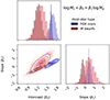 |
Fig. C.2. Same as Figure C.1, but for the Mp-Mz relation. |
| In the text | |
|
Fig. D.1. Heavy-element mass as a function of planet mass for the full (0.1 ≤ Mp(MJ)≤10, top) and limited samples (0.3 ≤ Mp(MJ)≤2, bottom). The scatter points and error bars show the inferred heavy-element mass by the thermal evolution models. Solid lines show the fits constructed by Bayesian regression, and the shaded contours are the one and two σ uncertainties. Planets around FGK stars are depicted in blue, while planets around M-dwarfs are orange and green depending on the age prior that was used (see text for details). |
| In the text | |
|
Fig. E.1. The residual normalised metallicity (the ratio of the calculated and predicted values) against various planetary and stellar properties. Planets around FGK and M-dwarf stars are depicted in blue circles and red hexagons. Filled symbols mark planets in the mass-limited sample (see text for further details). |
| In the text | |
|
Fig. E.2. The residual heavy-element mass (the ratio of the calculated and predicted values) against various planetary and stellar properties. Planets around FGK and M-dwarf stars are depicted in blue circles and red hexagons. Filled symbols mark planets in the mass-limited sample. See text for details. |
| In the text | |
Current usage metrics show cumulative count of Article Views (full-text article views including HTML views, PDF and ePub downloads, according to the available data) and Abstracts Views on Vision4Press platform.
Data correspond to usage on the plateform after 2015. The current usage metrics is available 48-96 hours after online publication and is updated daily on week days.
Initial download of the metrics may take a while.