| Issue |
A&A
Volume 693, January 2025
|
|
|---|---|---|
| Article Number | A116 | |
| Number of page(s) | 8 | |
| Section | Extragalactic astronomy | |
| DOI | https://doi.org/10.1051/0004-6361/202451153 | |
| Published online | 09 January 2025 | |
Explanations for the two-component spectral energy distributions of gravitationally lensed stars at high redshifts
1
Observational Astrophysics, Department of Physics and Astronomy, Uppsala University, Box 516 SE-751 20 Uppsala, Sweden
2
Swedish Collegium for Advanced Study, Linneanum, Thunbergsvägen 2, SE-752 38 Uppsala, Sweden
3
Department of Astronomy, University of Maryland, College Park, MD 20742, USA
4
Observational Cosmology Lab., NASA Goddard Space Flight Center, Greenbelt, MD 20771, USA
5
Instituto de Física de Cantabria (CSIC-UC), Avda. Los Castros s/n., 39005 Santander, Spain
⋆ Corresponding author; armin.nabizade@gmail.com
Received:
18
June
2024
Accepted:
6
November
2024
Observations of gravitationally lensed, high-mass stars at redshifts ≳1 occasionally reveal spectral energy distributions that contain two components with different effective temperatures. Given that two separate stars are involved, this suggests that both stars have simultaneously reached very high magnification, as expected for two stars in a binary system close to the caustic curve of the foreground galaxy-cluster lens. The inferred effective temperatures and luminosities of these stars are, however, difficult to reconcile with known binaries, or even with isolated stars of the same age. Here, we explore three alternative explanations for these cases: circumstellar dust around the cooler of the two stars, age differences of a few million years among stars in the same star cluster, and a scenario in which the stars originate in two separate star clusters of different age along the lensing caustic. While all of these scenarios are deemed plausible in principle, dust solutions would require more circumstellar extinction than seen in local observations of the relevant supergiant and hypergiant stars. Hence, we argue that age differences between the two stars are the most likely scenario, given the current data.
Key words: gravitational lensing: strong / gravitational lensing: micro / binaries: general / stars: massive / galaxies: star clusters: general
© The Authors 2025
 Open Access article, published by EDP Sciences, under the terms of the Creative Commons Attribution License (https://creativecommons.org/licenses/by/4.0), which permits unrestricted use, distribution, and reproduction in any medium, provided the original work is properly cited.
This article is published in open access under the Subscribe to Open model. Subscribe to A&A to support open access publication.
1. Introduction
In recent years, observations with the Hubble Space Telescope (HST) and the James Webb Space Telescope (JWST) of galaxy-cluster fields have enabled the detection of dozens of gravitationally lensed stars beyond the local Universe (Kelly et al. 2018, 2022; Chen et al. 2019, 2022; Kaurov et al. 2019; Welch et al. 2022a; Diego et al. 2023a,b; Meena et al. 2023; Yan et al. 2023; Fudamoto et al. 2024), with the highest-redshift example so far being the star Earendel at z ≈ 6 (Welch et al. 2022a,b). In some cases, the spectral energy distributions (SEDs) of these objects indicate the presence of two components with different effective temperatures (Teff), which has been interpreted as the blended light from two separate high-mass stars in the same star cluster or as two stars from a high-mass binary system (Welch et al. 2022b; Diego et al. 2023b; Furtak et al. 2024). However, the ratios of bolometric luminosities between the hot and cool components (possibly a blue supergiant and a yellow or red super- or hypergiant) inferred from the SED fits, are puzzling. In the two-component fits to lensed stars presented by Welch et al. (2022b), Diego et al. (2023b) and Furtak et al. (2024) the best-fitting bolometric luminosity ratios are Lhot/Lcool ≳ 2, which in the context of single-star evolution would be unexpected for two stars of the same age. A star with a higher initial mass is generally expected to evolve from high to low Teff at a faster pace and at a higher luminosity than a star with a lower initial mass. The latter is therefore expected to linger in a higher-Teff, lower-L state as the higher-mass star reaches its low-Teff, high-L end states, resulting in a bolometric luminosity ratio Lhot/Lcool ≲ 1 for two stars of the same age and metallicity.
The binary-star hypothesis may seem plausible, given that most high-mass stars are in binary systems (e.g. Offner et al. 2023; Sana et al. 2012), and at redshift z ≳ 1, only high-mass stars (≳5 − 10 M⊙) are likely to be rendered sufficiently bright by lensing to be detectable (Meena et al. 2022). Binary evolution can give rise to more complicated evolutionary pathways (for a recent review, see Marchant & Bodensteiner 2024), but in observed samples of red supergiants in binary systems (Patrick et al. 2022), cases where the hotter companion has a higher luminosity are very rare (in the sample of 88 red supergiant binaries in Patrick et al. 2022, all obey Lhot ≲ Lcold).
It is important to note that the empirical evidence supporting high binary fractions among massive stars is largely derived from observations within our galactic neighborhood. Consequently, when applying this knowledge to stellar populations at high redshifts, there is an implicit extrapolation. While this extrapolation is often considered reasonable, it should be acknowledged that the binary properties of massive stars at earlier cosmic times may differ due to varying environmental conditions, such as metallicity and star cluster density. Future observations are necessary to validate whether these trends hold in different epochs of the Universe.
In this work, we explore three alternative explanations for the luminosity anomaly observed in the two-component SEDs of lensed stars: (I) the possibility that the Lhot/Lcool ratio has been overestimated due to the presence of circumstellar dust around the low-Teff star in a same-age system; (II) the possibility that two stars that differ in age by a few million years may co-exist in the same star cluster, and (III) that the two stars are located in different star clusters, with more disparate ages, but still appear as an unresolved pair when lensed. Section 2 outlines the puzzle of the Lhot/Lcool luminosity ratios in lensed stars. Sections 3, 4, and 5 explore scenarios I, II, and III, respectively. Section 6 discusses and summarizes our findings and results.
2. The puzzling two-component SEDs of lensed stars
The current examples of lensed stars that may require two-component SED fits include Mothra at z ≈ 2 (Diego et al. 2023b), Earendel at z ≈ 6 (Welch et al. 2022a,b) and MACS0647-star-1 at z ≈ 5 (Meena et al. 2023; Furtak et al. 2024). In our view, Mothra provides the most robust case, because this object shows variability in the red component but not in the blue, which clearly demonstrates that (at least) two separate light sources must be contributing to the overall SED. The SED of Earendel reported by Welch et al. (2022b) is challenging to explain with the SED of a single star. However, it should be noted that all attempts to derive the photometry did not produce SEDs that would necessarily require such a solution (see Fig. 6 in Welch et al. 2022b). Furthermore, it is not clear whether the noisy JWST cycle-1 NIRSpec/prism spectrum of Earendel confirms the photometric SED (Welch et al., in prep.). Furtak et al. (2024) demonstrate that the JWST/NIRSpec spectrum of MACS0647-star-1 can be explained either as a two-component SED fit or a single, dust-reddened star. The possibility of it being an extreme star cluster is also suggested, although this explanation is disfavoured by the lensing situation.
What the SEDs of these lensed objects share in common is significant flux at wavelengths shortward of the Balmer break, with the break itself being very prominent for Earendel and MACS0647-star-1, and less so for Mothra. However, they exhibit a relatively flat continuum longward of the break. The former is, broadly speaking, expected for a star with Teff > 10 000 K (the blue continuum slope of Earendel shortward of the Balmer break moreover requires Teff > 20 000 K), whereas the latter is expected for a Teff < 8000 K star. Since the Thot, Tcool and Lhot/Lcool solutions of these objects exhibit substantial degeneracies, we will assume throughout this paper that acceptable solutions have Thot > 12 000 K, Tcool < 8000 K, and Lhot/Lcool ≥ 2.
Given typical stellar evolutionary tracks for single stars, solutions that match these criteria require very finely tuned ages and masses if one needs the two stars to have formed at the same time. This is exemplified using SMC-metallicity tracks from Szécsi et al. (2022), and isochrones derived from these, in Fig. 1. For this set of tracks, solutions are possible in cases where the more massive, higher-L star evolves back in the blueward direction towards high Teff after a brief time in a lower-Teff state. If a lower-mass, lower-luminosity star simultaneously happens to have evolved to low Teff, the required Thot, Tcool, and Lhot/Lcool conditions can in principle be met.
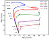 |
Fig. 1. Evolutionary tracks for various ZAMS masses obtained from the BoOST SMC (gray dashed lines; Szécsi et al. 2022) stellar evolutionary tracks, together with the corresponding isochrones interpolated for selected ages (colored solid lines). In this set of stellar evolutionary tracks, cases where two stars along the same isochrone may exhibit Thot > 12 000 K, Tcool < 8000 K, and Lhot/Lcool ≥ 2 arise only at ages ≲3 Myr, where the isochrones curve back towards high Teff (red and blue lines) due to blueward evolution along the MZAMS > 55 M⊙ tracks. |
By investigating isochrones between 1 and 27 Myr, separated by 0.1 Myr, we identified solutions for four isochrones at ages 2.4, 2.5, 2.6, and 2.7 Myr where cold and hot components can exhibit Lhot/Lcool ≥ 2. This is consistent with the fact that extremely massive stars, for which L ∼ Ledd, have lifetimes of approximately 3 Myr. Two such solutions are shown in Fig. 2. These solutions require a cold component with a Zero Age Main-Sequence (ZAMS) mass ∼83 − 105 M⊙ and a hot component with a ZAMS mass in range ∼121 − 176 M⊙ which corresponds to a narrow mass ratio of RM = MZAMS, cold/MZAMS, hot = 0.58 − 0.68. The limited number of isochrones and the narrow range of ZAMS masses yielding acceptable solutions indicate that such cases must be exceedingly rare (solutions in only 4 isochrones out of 270 studied matched the criteria). This demonstrates why it generally appears unlikely for two massive stars (ZAMS mass M ≥ 9 M⊙) of the same age to account for the observed two-component SEDs of lensed stars under the assumption of single-star evolution, in cases where they are two genuine single stars from a star cluster, where all stars have the same age, or members of a non-interacting binary system.
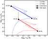 |
Fig. 2. Examples of BoOST SMC Isochrones for which the Thot > 120 00 K, Tcool < 8000 K, and Lhot/Lcool ≥ 2 conditions for lensed stars with two-component SEDs can be met. The isochrones are depicted with the blue and red dashed lines, obtained for ages 2.4 and 2.7, respectively. The blue and red solid lines connect stars with the same ages and different ZAMS masses that meet the requirements. For clarity, the red isochrone has been shifted downward, as indicated by the black arrow. |
The other possibility is that the composite SED emerges from two stars in an interacting binary. Stars in close interacting binaries may exhibit radically different evolutionary paths, since the rapid rotation–whether primordial or due to tidal locking in a close binary system–can cause the faster-evolving stars to shift blueward toward higher Teff, rather than redward toward lower Teff. Furthermore, in interacting binaries, the accretor can become overluminous during the accretion process (Sen et al. 2023), while the donor may become underluminous (Renzo & Götberg 2021; Pauli et al. 2022). This imbalance can potentially result in a SED that matches our Teff and Lhot/Lcool criteria. To investigate this, we used the Binary Population and Spectral Synthesis (BPASS) models v2.2 (Stevance et al. 2020) across metallicities ranging in Z = 0.001 − 0.040, along with the HOKI Python package1 (Stevance et al. 2020). For solar metallicities and below, no systems matching our criteria were found. For Z = 0.02 − 0.03, a small number of solutions did emerge, but only for stars with bolometric luminosities log10(L/L⊙) < 4.4. Such stars are generally too faint to match the observed cases of two-component lensed stars without uncomfortably high magnifications (≳30 000 in the case of Mothra; Diego et al. 2023b). A larger number of acceptable solutions were found to exist at metallicities Z ∼ 0.04, but in the high-redshift Universe, stars with such high metallicities are likely to be very rare.
3. Scenario I: Circumstellar dust around the low-Teff component
A potential explanation for the anomalous luminosity ratios observed between the two SED components in lensed stars such as Mothra and Earendel is that the constituent stars have the same age, but the low-Teff star experiences more extinction compared to the high-Teff star. If this scenario is overlooked during the fitting procedure, where observed SEDs are fitted to models assuming equal or no extinction for both stars, this results in an underestimation of the luminosity of the low-Teff-pagination object.
In a scenario where the two stars are members of the same star cluster, regardless of whether they are also part of the same binary system, they may potentially experience comparable levels of extinction from both the interstellar medium within the cluster and the ambient interstellar medium of the host galaxy. However, if the stars are not in the same binary system, and one of the stars has been actively producing dust in its immediate surroundings, the SED of that star may experience an additional, potentially dominant extinction component, which dims its apparent brightness. Both red supergiants and yellow supergiants are known to be surrounded by circumstellar dust, sometimes resulting in several magnitudes of visual extinction (e.g. Massey et al. 2005; Gordon et al. 2016). One example of a star where dust extinction is blamed for dimming is R Coronae Borealis, where varying dust extinction causes an apparent luminosity change of over 8 mag (O’Keefe 1939). Here, we investigate the extent to which solutions involving circumstellar dust around the low-Teff component can explain the properties of Mothra.
As discussed in Diego et al. (2023b), the long-wavelength part of the Mothra SED displays significant variability for observed wavelengths ≳1.5 μm, whereas the short-wavelength part does not. The observed variability coupled with the lower redshift of Mothra, enables the existing JWST/NIRCam observations to probe the SED at rest-frame near-infrared wavelengths. This provides stronger constraints to be placed on the nature of the low-Teff component compared to Earendel. In Yan et al. (2023), the JWST/NIRCam SEDs for Mothra are presented at three separate epochs, in which the long-wavelength component displays the lowest brightness in epoch 1 and the highest in epoch 3. These epochs are separated by ≈126 days in the observed frame, corresponding to a rest-frame variability timescale of ≈41 days at the redshift of Mothra, under the assumption that the variability is entirely intrinsic to the source and not affected by changes in microlensing magnification between the two components.
In Fig. 3, we demonstrate that by combining the HST observation of Diego et al. (2023b) with the JWST observation of epochs 1 and 3 from Yan et al. (2023), it is possible to find acceptable SED fits that include circumstellar dust around the low-Teff star and results in a non-anomalous intrinsic luminosity ratio of Lhot/Lcool ≈ 0.74. This SED solution is however, not unique, as it is possible to match both the overall SED and its change over time with models that allow variations in circumstellar dust extinction, luminosity, effective temperature, or some combination thereof, between the epochs. The solution shown in Fig. 4 assumes the circumstellar extinction remains constant between the observed epochs, and follows a Milky Way reddening law (RV = AV × E(B − V) = 3.1) as parameterized by Li et al. (2008) in the Mothra rest frame.
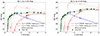 |
Fig. 3. Effect of including circumstellar dust around the cooler component in the two-star solution for the observed Mothra SED. Two fits have been conducted for the SEDs, corresponding to epoch 1 (left) and epoch 3 (right), considering the variability of the cooler component. In the fits presented, the effective temperature and luminosity of the cooler component are both allowed to vary between the epochs. As seen, significant circumstellar extinction (here AV = 2.8 mag) allows for good fits to the SEDs of both epochs while keeping Lhot/Lcool < 1. |
Including circumstellar dust in the fit has the effect of raising the intrinsic luminosity of the low-Teff component. Additionally, assuming a non-gray extinction law (i.e., one that produces reddening) also increases the effective temperature (Teff) of the best-fitting low-Teff component compared to a fit that assumes negligible extinction. In the extinction-free fit presented by Diego et al. (2023b), but with otherwise identical SED models, the effective temperature of the low-Teff model was 5250 K. In our analysis, we infer temperatures of 7500 K in epoch 1 and a drop of 500 K by epoch 3, with a luminosity that increases by a factor of approximately 1.8 between the epochs. This solution roughly matches the Teff and luminosity variations of yellow supergiants and hypergiants (e.g. Percy & Kim 2014; van Genderen et al. 2019). However, the required circumstellar extinction is very high (AV = 2.8 mag) compared to the majority of such objects, where a total visual dust extinction of AV ≲ 2 is more common (Gordon et al. 2016; Humphreys et al. 2023), and the amount of interstellar extinction affecting both components is very low (AV = 0 mag in the presented fit, although up to ≈0.3 mag can be accommodated).
Acceptable fits can also be found when only the extinction and effective temperature are kept fixed while allowing only the luminosity to vary between epochs. The increase in luminosity between epochs changes to a factor of approximately 2, which is comparable to the factor obtained when the effective temperature was allowed to vary alongside the luminosity. However, allowing only the effective temperature or only the circumstellar dust extinction to vary between the epochs does not yield any viable solutions.
We conclude that while a solution that includes circumstellar dust extinction can reduce the anomalous Lhot/Lcool luminosity ratio, the significant amount of extinction required makes it challenging to reconcile the low-Teff star with the supergiants and hypergiants observed in the local Universe.
4. Scenario II: Two stars from the same star cluster
Two stars do not necessarily need to form a binary system to attain very high magnifications simultaneously. Typically, it is sufficient for them to be projected within ≲1 pc of the macrocaustic of a strong-lensing galaxy cluster to reach a total magnification of ≳1000. Considering that at z ≳ 1 only young, high-mass stars can be rendered detectable by lensing, and given the highly clustered nature of star formation, it seems reasonable to assume that if a highly magnified star is detected, there are likely other high-mass stars in its vicinity. This holds true in cases where the stars are born as members of a bound star cluster, but it may also apply temporarily even if they are formed as part of a dispersing open cluster or OB association. Well-studied young, resolved star clusters like the Orion Nebula Cluster and R136 do indicate an age spread of a few million years within a 1 pc radius (e.g. Krumholz et al. 2019; Bestenlehner et al. 2020). Whether this age spread is intrinsic to these clusters in three dimensions or is a result of contamination by background and/or foreground stars within an extended star-forming complex where these clusters reside is not that important in the current context. What matters instead is the projected age distribution at small separations in the plane of the sky that affects the lensing situation.
Hence, we explored whether two stars with ZAMS mass in the range of 9 − 498 M⊙ at ages up to 27.6 Myr from the same star cluster, with the same metallicity, but with a small age difference may explain the Lhot/Lcool conundrum. Considering the previous conditions, we searched for pairs of solutions among different isochrones with an age difference of up to 3 Myr, derived from the Szécsi et al. (2022) SMC-metallicity tracks. This resulted in a wider mass ratio range for the pair solutions of RM = 0.07 − 0.89. A few examples of such solutions for various ages and masses are shown in Fig. 4.
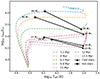 |
Fig. 4. Same as Fig. 2 but for the stars with an age difference of ≤3 Myr. In this case, more numerous combinations of stars –within wider age and mass ranges – meet the Lhot/Lcool > 2 and Teff requirements for the two-component SEDs. Here, only a few examples together with their ZAMS masses are shown. |
To investigate how the age difference between two stars affects the probability of finding such solutions, we performed a simple calculation based on a stellar initial mass function with slope dN/dM ∝ M−2.3, as suggested by Kroupa (2001) for MZAMS ≥ 1 M⊙. Under the assumption that the age distribution within a star cluster is uniform up to Δ(t) = 3 Myr, and that all star-cluster ages are equally likely, we find that the likelihood of encountering these solutions in a star cluster increases by a factor of ≈260, compared to the single-age star cluster case. While this calculation may not accurately capture the likelihood of observing these solutions in samples of lensed stars, which are subject to additional biases related to the magnification distribution, bolometric luminosities, Teff and radii of stars (Zackrisson et al. 2024), it does lend credence to the idea that stars from the same star cluster – but with slightly different ages – offers a viable solution to the Lhot/Lcool problem.
While the models for interacting binary stars used in this work (see Section 2) did not provide much support for the notion that an individual interacting binary system would be able to explain the observed properties of lensed stars with two-component SEDs, scenarios may still be considered in which interacting binary stars are in some way involved in the solution. For instance, one component from an interacting binary could end up projected close to an unrelated, single star within the same cluster, thereby experiencing a similar magnification. While such configurations would formally involve three stars, the subdominant component of the binary may not contribute sufficiently to the observed SED to be noticeable given the typical data quality for lensed stars at high redshifts. Similarly, situations involving two interacting binaries (four stars) projected close to each other could also be considered. While we have not explored such models in detail, it is possible that such configurations would be able to provide viable SED solutions with smaller age differences between the stars than in cases involving two single stars. Observationally confirming such cases would, however, be very challenging, as discussed in Section 6.
5. Scenario III: Two stars from different star clusters
The analysis of the two-component SEDs by Welch et al. (2022a,b), Diego et al. (2023b), Furtak et al. (2024) assumes that the two stars would be projected within < 1 pc of each other in the source plane, but this is not the only possibility. In Figure 5 we schematically illustrate the case where one star is placed at various distances along the direction perpendicular to the macrolensing caustic curve in the source plane. At the largest separation from the caustic, this results in two distinct and well-separated images with intermediate magnification in the image plane. As the distance to the caustic decreases, these images become closer together and more highly magnified and eventually start to blend in the image plane (images 1a and 1b in Figure 5). However, if a second star is placed similarly close to the caustic, but at a separation of up to ≈100 pc along the caustic, a second pair of images (4a and 4b) will appear extremely close to the first pair (1a and 1b), potentially appearing as an unresolved source at the angular resolution of JWST images. This is a consequence of the modest value for the component of the magnification located in the direction along the caustic, μr, which typically takes values between 1 and 2, while the component of magnification in the direction perpendicular to the caustic of the magnification, μt, can take much larger values, and exceeding 1000 close enough to the caustic. Hence objects near the caustic get amplified by a much larger factor μt in the direction perpendicular to the caustic than in the direction along the caustic, and two objects separated by a substantial distance in the direction along the caustic can remain unresolved when amplified.
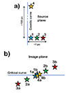 |
Fig. 5. Schematic illustration of the lensing situations that allow the light from two stars in separate star clusters to blend together in the image plane forming a two-component SED. (a) The situation in the source plane, with three stars (1, 2 and 3) located close to each other and within ∼1 pc of the caustic curve. A fourth star (4) is located at a similar distance from the caustic as 1, but up to ≈100 pc away in the direction along the caustic. (b) The corresponding image-plane situation, where the stars 2 and 3 appear as resolved double images (2ab, 3ab) with a separation that increases with their distance from the caustic in (a). The images of stars 1 and 4, on the other hand, form two sets of overlapping image pairs (1ab and 4ab) at very high magnification, separated by only a small distance from the critical curve. Since the radial magnification μr is much smaller than the tangential magnification μt along the critical curve (by a factor of μr/μt ≲ 0.01), the two image pairs 1ab and 4ab may appear as an unresolved source at the angular resolution of JWST. |
To date, the strongest constraints on the separation between the two stars contributing to SEDs of lensed stars come from Welch et al. (2022b) for the z ≈ 6 star Earendel (< 0.02 pc). This constraint is based on simulations of the type shown in Welch et al. (2022a), where the separation of two-point sources is increased until the resulting image of stars becomes resolvable and no longer matches the observed point-like morphology. However, these simulations assumed the separation to be in the direction perpendicular to the caustic, rather than along the caustic. By rerunning the simulations, assuming Earendel to cover ≤1 native detector pixel (0.031 arcsec for the NIRCam short-wavelength images) with the separation along the caustic for five different lens models, we obtained the upper limits on the separation presented in Table 1, which are in the range 85−160 pc.
Maximum separation along the caustic between two point sources contributing to the unresolved JWST morphology of Earendel (Welch et al. 2022b).
This demonstrates the viability of solutions to the two-component SED conundrum in which the two massive stars are separated by up to ≈100 pc and hence likely belong to different star clusters and potentially different star-forming regions. In such scenarios, the ages, magnifications and potentially even metallicities of the two stars may differ significantly. Since both stars are likely to have a very high ZAMS mass (≳20 M⊙ in the case of Earendel; Welch et al. 2022b), they must both originate from young star clusters.
Given that we know there must be at least one such cluster close to the caustic, the probability that there is another one within ≈100 pc along the caustic needs to be determined.
In the following, we assess the probability that more than one star-cluster is present within the JWST PSF of a strongly magnified object at z ∼ 6 − 10. To quantify this effect, we use a simulation presented in Garcia et al. (2023), in which the high star formation efficiency (HSFE run) of the star-forming clouds leads to the formation of compact (radii of ∼1 − 2 pc) and gravitationally bound star clusters. The choice is justified by the qualitative agreement between the clumpiness of these simulated high-redshift galaxies (see also, Sugimura et al. 2024) and observations of strongly lensed arcs at z > 6 (Welch et al. 2022a; Adamo et al. 2024; Bradley et al. 2024). This is illustrated in Figure 6, showing a snapshot of one of these galaxies (left panel) and the lensed arc it produces (right panel) when using the lens model for the Sunrise Arc/Earendel (Welch et al. 2022a). The left panel shows the distribution of the stars in the galaxy, which appear as a collection of bound star clusters, with no prominent bulge or disk. The color coding shows the surface density of the stars projected on the sky; the scale, in parsecs, is shown by the inset white bar, while the yellow rectangle of dimensions 1 pc × 100 pc represents the JWST pixel near the critical curve, traced back to the source plane.
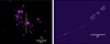 |
Fig. 6. Left: Snapshot of a simulated high-z galaxy from Garcia et al. (2023) (HSFE run). In this simulation, the high star formation efficiency (HSFE) in its star-forming gas clouds, which have densities ∼100× that of Milky Way’s molecular clouds, leads to the formation of numerous compact (radii of ∼1 − 2 pc) and gravitationally bound star clusters. Here the color coding shows the density of stars and the yellow rectangle of size 1 × 100 pc represents a sketch of a ray-traced JWST pixel next to the critical curve (line of infinite magnification) traced from the image plane to the source plane (left). The location of the galaxy with respect to the yellow rectangle (arbitrarily chosen in this figure) is randomized in order to assess the magnification probability of N star clusters. Right: Lensed image of the galaxy shown on the left panel, placed at z = 6 across the caustic of the cluster WHL0137-08, using the GLAFIC lensing model reproducing the Sunrise Arc/Earendel. We labeled only the clumps that are mirror images around the location of Earendel. See the text for the details of how the image was produced. |
The right panel shows the observed flux of the galaxy produced by the stellar continuum at 1500 Å (rest frame), using the GLAFIC lens model for the Sunrise Arc (Welch et al. 2022a) with the simulated galaxy placed at z = 6 next to the caustic. The scale of the arc, in arcseconds, is indicated by the inset white bar. We note that the linear scale of the galaxy has been increased by a factor of two to match the size and stellar mass (scaled up by a factor 24) of the z = 6 galaxy producing the Sunrise Arc. With this scaling, we reproduced the total stellar mass and extent of the arc, as well as its observed flux and clumpiness. Further details on the ray tracing method and the Python package used to create this image will be published in Park et al. (in preparation). In the simulations by Garcia et al. (2023), star particles have masses of 10 M⊙ and bound star clusters have a power-law mass function with a slope of Γ ∼ −1.5 ± 1 and masses ranging between 500 M⊙ and 5 × 10⁴ M⊙. A flatter slope, close to Γ = −0.5 is found in simulations with a more bursty star formation and a clumpy appearance, while a steeper slope is associated with less bursty and more diffuse galaxies. After the scaling mentioned above the masses increase by a factor of about 20 to 104 M⊙ − 106 M⊙.
The histogram in Fig. 7 shows the probability that the light in a strongly magnified pixel near the caustic is produced by a number N ≥ 1 of star clusters. We used the following procedure to obtain the histogram. Initially, we used a single snapshot from the simulation (the one shown in Fig. 6). We created 50 000 random realizations for the position and rotation of the galaxy relative to the 1 × 100 pc rectangle. For each realization, we then created a 1D histogram of the star counts falling within it, as a function of the position along its longer side. We smoothed the histogram using a Gaussian kernel with a σ = 0.1 pc and estimated the number of star clusters by counting the number of peaks above a threshold of 4. We also remove stars older than 10 Myr as they would have a negligible contribution to the luminosity and discarded realizations with a total number of stars within the rectangle less than 200, for the same reason. Finally, we produced a histogram of occurrences of N star clusters and normalized it to unity after removing the bin with N = 0. We have also done the same calculation including a few hundred snapshots at various cosmic times for the same simulation. However, for the sake of brevity, we do not show this case since the resulting histogram is almost identical to the one shown here.
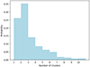 |
Fig. 7. Probability distribution (normalized to unity) that N star clusters (excluding the cases with N = 0) are within 1 pc of the caustic (line of infinite magnification on the source plane) for the different realization of the position and rotation of the galaxy shown in Fig. 1. The histogram shows that if enough stars are present near the caustic the probability they are all in a single star cluster is P(1) = 25%, while the probability of them being in two clusters is higher (P(2) = 35% or P(2)/P(1) = 1.4). The probability of them being in more than one cluster (2 and above) is ∼75%. |
Fig. 7 shows that if enough stars are present near the caustic the probability they are all within one star cluster is P(1) = 25%, while the probability of them being in two distinct clusters is higher (P(2) = 35% or P(2)/P(1) = 1.4). Overall the probability of them being in more than one cluster (i.e., two or more) is ∼75%, hence very likely.
If we think in terms of a mathematically motivated model for the distribution, assuming that the star clusters are not clustered (i.e., randomly distributed in the sky) we can describe the probability of N star clusters being present in a region of area A within the whole galaxy of area B as Binomial:
where n is the total number of star clusters in the galaxy and the probability p = A/B is the fraction of the projected area of the galaxy covered by the JWST pixel next to the caustic on the source plane, represented by the yellow rectangle 1 pc × 100 pc = 100 pc2 shown in Figure 6-left. A rough estimate for p, accounting for a diameter of the star clusters of 5 pc is p ≈ 1000/105 ≈ 10−2. The typical number of star clusters in the galaxy is about 100 (including the low-mass end of the distribution), hence the mean of the distribution is np ∼ 1 − 2 and the peak (mode) is ⌊(n + 1)p⌋≈1 − 2. Since n is reasonably large we can approximate the Binomial with a Poisson distribution:
where λ = np ∼ 1 − 2. The probability P(2)/P(1) = np/2 ∼ 0.5 − 1. From the simulations we find an even larger ratio, probably because our assumption of a random distribution for the star cluster within the galaxy is incorrect: inspecting Fig. 6-left it is evident that star clusters show significant clustering.
Given that it seems quite likely that more than one young, massive star cluster is located close to the caustic, and that the probability of finding solutions that explain the Lhot/Lcold problem of lensed stars with two-component SEDs increases when the ages of the stars are allowed to vary (Section 4), we argue that this scenario (III) is the most likely out of the ones explored.
6. Discussion and conclusion
The search for high-redshift lensed stars through HST and JWST observations has revealed a few cases with two-component SEDs, where both a cold and a hot component are involved with Lhot/Lcool ≳ 2. Given that the two-component SED emerges from a blue supergiant and a yellow or red supergiant, this ratio is unlike that of two stars of the same age, in the context of single-star evolution.
One may envision scenarios in which the merger of two stars forms a rejuvenated, high-Teff and high-L object (e.g. Glebbeek et al. 2013; Wang et al. 2022), which could then be lensed to detectable levels together with an unrelated lower-L star from the same star cluster. If this merger happens in what was originally a triple-star system, the merger product could also potentially find itself bound to a cooler low-L star in a binary. However, if such cases were common, it remains unclear why such stars would not turn up more often in local samples of red supergiant binaries.
In this study, we investigated the possible explanations for this luminosity ratio discrepancy by examining three different scenarios:
-
High intrinsic extinction of the low-Teff component due to circumstellar dust may lower its apparent luminosity, which – if not corrected for – leads to an increase in Lhot/Lcool. However, this would require a substantial amount of such dust around the red component, likely a supergiant or a hypergiant, a condition not commonly observed in the local Universe.
-
The observed SED of a magnified object might indeed result from two stars located in the same star cluster (see Sect. 4). However, since stars within a star cluster are generally of similar ages, the number of pair solutions decreases as the age difference (Δt) between the stars becomes smaller.
-
On the other hand, based on the simulations described above, there is a considerable chance of the stars originating in different star clusters close to the caustic curve, with a separation distance of up to 100 pc along the caustic. Given this scenario, two stars with an age difference ≲30 Myr (the maximum lifetime of ≳10 M⊙ stars), can both become lensed, resulting in an unresolved magnified image where the observed SED would exhibit a dual-component nature.
It is important to note that in examining Scenario II, the Szécsi et al. (2022) stellar tracks we used in this work include systematic uncertainties that could impact the resulting isochrones. Specifically, the evolutionary tracks for a single star rely on a set of fixed assumptions regarding the star’s envelope physics, including factors such as envelope inflation (Paxton et al. 2013; Agrawal et al. 2020) and mass loss rate (Smith 2014; Cheng et al. 2024), among others. It is hence possible that a grid covering a wider range of parameters would allow a greater number of solutions for same-age pairs of single stars.
Among the three different scenarios we studied here, the third one is more favorable. This scenario, supported by simulations, would explain the two-component spectra of high-z lensed stars, such as Mothra and Erendal. The observed spectra in this scenario, which are a combination of two individual spectra originating from two stars located in different star clusters, could provide a solid explanation for the observed distinct characteristics such as age, luminosity, and temperature. This suggests that the lensed sources might not necessarily be binary systems.
One potential way to observationally differentiate between the different scenarios would be to try to spectroscopically measure the difference in projected velocity difference between the two stars through their absorption lines. Spectroscopy of lensed stars is in general very challenging due to the faintness of the majority of such objects, and stellar absorption lines can for mAB ≳ 26 AB mag stars realistically only be done at spectral resolution R ∼ 1000 with JWST and ∼3000 with ELT (Lundqvist et al. 2024). At the relatively low signal-to-noise levels of the Lundqvist et al. (2024) simulated spectra (even at very long exposure times; 50 h for JWST and 10 h for ELT), velocity differences below the spectral FWHM are difficult to discern, which means that projected velocities below ∼300 km s−1 (JWST) and ∼100 km s−1 (ELT) are likely to be undetected even if both stars display detectable absorption lines.
In our star cluster models (Section 5), the one-dimensional velocity differences between two single stars from different star clusters is only ∼10 km s−1 (this takes into account both the internal velocity dispersion within each cluster and the motion of star cluster with respect to each other). Hence, if we see two single stars in two different star clusters, we do not expect to be able to measure any velocity difference between the stars. However, the velocity amplitudes of some massive-star binary systems do reach ≳100 km s−1 (Kobulnicky et al. 2014), which means that if either of the two stars involved in the two-star SEDs of lensed stars is part of a binary system, we may be able to tell from spectra taken at different epochs.
Unfortunately, simply detecting a change in velocity between the two stars may not be very informative. The important question is whether the two stars that dominate the two-component SEDs of lensed stars are located in the same binary system, but since most massive stars are expected to be in binary systems anyway, a velocity shift over time between the two components may for instance also allow for models in which two stars are the brightest members of two separate binary systems, either located in the same star cluster or in two different star clusters. Getting the orbital constraints required to disentangling such scenarios may require many epochs of data, which would be extremely expensive in terms of observing time.
Acknowledgments
AN and EZ acknowledge funding from Olle Engkvists Stiftelse. EZ also acknowledges grant 2022-03804 from the Swedish Research Council, and has benefited from a sabbatical at the Swedish Collegium for Advanced Study. JMD acknowledges support from project PID2022-138896NB-C51 (MCIU/AEI/MINECO/FEDER, UE) Ministerio de Ciencia, Investigación y Universidades. We would also like to thank the referee for thoroughly reading our manuscript and providing valuable comments that contributed to enhancing the quality of the paper.
References
- Adamo, A., Bradley, L. D., Vanzella, E., et al. 2024, Nature, 632, 513 [NASA ADS] [CrossRef] [Google Scholar]
- Agrawal, P., Hurley, J., Stevenson, S., Szécsi, D., & Flynn, C. 2020, MNRAS, 497, 4549 [NASA ADS] [CrossRef] [Google Scholar]
- Bestenlehner, J. M., Crowther, P. A., Caballero-Nieves, S. M., et al. 2020, MNRAS, 499, 1918 [Google Scholar]
- Bradley, L. D., Adamo, A., Vanzella, E., et al. 2024, ArXiv e-prints [arXiv:2404.10770] [Google Scholar]
- Chen, W., Kelly, P. L., Diego, J. M., et al. 2019, ApJ, 881, 8 [NASA ADS] [CrossRef] [Google Scholar]
- Chen, W., Kelly, P. L., Treu, T., et al. 2022, ApJ, 940, L54 [NASA ADS] [CrossRef] [Google Scholar]
- Cheng, S. J., Goldberg, J. A., Cantiello, M., et al. 2024, ApJ, 974, 270 [NASA ADS] [CrossRef] [Google Scholar]
- Diego, J. M., Meena, A. K., Adams, N. J., et al. 2023a, A&A, 672, A3 [NASA ADS] [CrossRef] [EDP Sciences] [Google Scholar]
- Diego, J. M., Sun, B., Yan, H., et al. 2023b, A&A, 679, A31 [NASA ADS] [CrossRef] [EDP Sciences] [Google Scholar]
- Fudamoto, Y., Sun, F., Diego, J. M., et al. 2024, ArXiv e-prints [arXiv:2404.08045] [Google Scholar]
- Furtak, L. J., Meena, A. K., Zackrisson, E., et al. 2024, MNRAS, 527, L7 [NASA ADS] [Google Scholar]
- Garcia, F. A. B., Ricotti, M., Sugimura, K., & Park, J. 2023, MNRAS, 522, 2495 [NASA ADS] [CrossRef] [Google Scholar]
- Glebbeek, E., Gaburov, E., Portegies Zwart, S., & Pols, O. R. 2013, MNRAS, 434, 3497 [NASA ADS] [CrossRef] [Google Scholar]
- Gordon, M. S., Humphreys, R. M., & Jones, T. J. 2016, ApJ, 825, 50 [NASA ADS] [CrossRef] [Google Scholar]
- Humphreys, R. M., Jones, T. J., & Martin, J. C. 2023, AJ, 166, 50 [NASA ADS] [CrossRef] [Google Scholar]
- Kaurov, A. A., Dai, L., Venumadhav, T., Miralda-Escudé, J., & Frye, B. 2019, ApJ, 880, 58 [NASA ADS] [CrossRef] [Google Scholar]
- Kelly, P. L., Diego, J. M., Rodney, S., et al. 2018, Nat. Astron., 2, 334 [NASA ADS] [CrossRef] [Google Scholar]
- Kelly, P. L., Chen, W., Alfred, A., et al. 2022, ArXiv e-prints [arXiv:2211.02670] [Google Scholar]
- Kobulnicky, H. A., Kiminki, D. C., Lundquist, M. J., et al. 2014, ApJS, 213, 34 [Google Scholar]
- Kroupa, P. 2001, MNRAS, 322, 231 [NASA ADS] [CrossRef] [Google Scholar]
- Krumholz, M. R., McKee, C. F., & Bland-Hawthorn, J. 2019, ARA&A, 57, 227 [NASA ADS] [CrossRef] [Google Scholar]
- Li, A., Liang, S. L., Kann, D. A., et al. 2008, ApJ, 685, 1046 [NASA ADS] [CrossRef] [Google Scholar]
- Lundqvist, E., Zackrisson, E., Hawcroft, C., Amarsi, A. M., & Welch, B. 2024, A&A, 690, A291 [NASA ADS] [CrossRef] [EDP Sciences] [Google Scholar]
- Marchant, P., & Bodensteiner, J. 2024, ARA&A, 62, 21 [NASA ADS] [CrossRef] [Google Scholar]
- Massey, P., Plez, B., Levesque, E. M., et al. 2005, ApJ, 634, 1286 [NASA ADS] [CrossRef] [Google Scholar]
- Meena, A. K., Arad, O., & Zitrin, A. 2022, MNRAS, 514, 2545 [CrossRef] [Google Scholar]
- Meena, A. K., Zitrin, A., Jiménez-Teja, Y., et al. 2023, ApJ, 944, L6 [NASA ADS] [CrossRef] [Google Scholar]
- Offner, S. S. R., Moe, M., Kratter, K. M., et al. 2023, ASP Conf. Ser., 534, 275 [NASA ADS] [Google Scholar]
- O’Keefe, J. A. 1939, ApJ, 90, 294 [CrossRef] [Google Scholar]
- Patrick, L. R., Thilker, D., Lennon, D. J., et al. 2022, MNRAS, 513, 5847 [Google Scholar]
- Pauli, D., Langer, N., Aguilera-Dena, D. R., Wang, C., & Marchant, P. 2022, A&A, 667, A58 [NASA ADS] [CrossRef] [EDP Sciences] [Google Scholar]
- Paxton, B., Cantiello, M., Arras, P., et al. 2013, ApJS, 208, 4 [Google Scholar]
- Percy, J. R., & Kim, R. Y. H. 2014, J. Am. Assoc. Var. Star Obs., 42, 267 [NASA ADS] [Google Scholar]
- Renzo, M., & Götberg, Y. 2021, ApJ, 923, 277 [NASA ADS] [CrossRef] [Google Scholar]
- Sana, H., de Mink, S. E., de Koter, A., et al. 2012, Science, 337, 444 [Google Scholar]
- Sen, K., Langer, N., Pauli, D., et al. 2023, A&A, 672, A198 [NASA ADS] [CrossRef] [EDP Sciences] [Google Scholar]
- Smith, N. 2014, ARA&A, 52, 487 [NASA ADS] [CrossRef] [Google Scholar]
- Stevance, H., Eldridge, J., & Stanway, E. 2020, J. Open Source Softw., 5, 1987 [NASA ADS] [CrossRef] [Google Scholar]
- Sugimura, K., Ricotti, M., Park, J., Garcia, F. A. B., & Yajima, H. 2024, ApJ, 970, 14 [NASA ADS] [CrossRef] [Google Scholar]
- Szécsi, D., Agrawal, P., Wünsch, R., & Langer, N. 2022, A&A, 658, A125 [NASA ADS] [CrossRef] [EDP Sciences] [Google Scholar]
- van Genderen, A. M., Lobel, A., Nieuwenhuijzen, H., et al. 2019, A&A, 631, A48 [NASA ADS] [CrossRef] [EDP Sciences] [Google Scholar]
- Wang, C., Langer, N., Schootemeijer, A., et al. 2022, Nat. Astron., 6, 480 [NASA ADS] [CrossRef] [Google Scholar]
- Welch, B., Coe, D., Diego, J. M., et al. 2022a, Nature, 603, 815 [NASA ADS] [CrossRef] [Google Scholar]
- Welch, B., Coe, D., Zackrisson, E., et al. 2022b, ApJ, 940, L1 [NASA ADS] [CrossRef] [Google Scholar]
- Yan, H., Ma, Z., Sun, B., et al. 2023, ApJS, 269, 43 [NASA ADS] [CrossRef] [Google Scholar]
- Zackrisson, E., Hultquist, A., Kordt, A., et al. 2024, MNRAS, 533, 2727 [NASA ADS] [CrossRef] [Google Scholar]
All Tables
Maximum separation along the caustic between two point sources contributing to the unresolved JWST morphology of Earendel (Welch et al. 2022b).
All Figures
|
Fig. 1. Evolutionary tracks for various ZAMS masses obtained from the BoOST SMC (gray dashed lines; Szécsi et al. 2022) stellar evolutionary tracks, together with the corresponding isochrones interpolated for selected ages (colored solid lines). In this set of stellar evolutionary tracks, cases where two stars along the same isochrone may exhibit Thot > 12 000 K, Tcool < 8000 K, and Lhot/Lcool ≥ 2 arise only at ages ≲3 Myr, where the isochrones curve back towards high Teff (red and blue lines) due to blueward evolution along the MZAMS > 55 M⊙ tracks. |
| In the text | |
|
Fig. 2. Examples of BoOST SMC Isochrones for which the Thot > 120 00 K, Tcool < 8000 K, and Lhot/Lcool ≥ 2 conditions for lensed stars with two-component SEDs can be met. The isochrones are depicted with the blue and red dashed lines, obtained for ages 2.4 and 2.7, respectively. The blue and red solid lines connect stars with the same ages and different ZAMS masses that meet the requirements. For clarity, the red isochrone has been shifted downward, as indicated by the black arrow. |
| In the text | |
|
Fig. 3. Effect of including circumstellar dust around the cooler component in the two-star solution for the observed Mothra SED. Two fits have been conducted for the SEDs, corresponding to epoch 1 (left) and epoch 3 (right), considering the variability of the cooler component. In the fits presented, the effective temperature and luminosity of the cooler component are both allowed to vary between the epochs. As seen, significant circumstellar extinction (here AV = 2.8 mag) allows for good fits to the SEDs of both epochs while keeping Lhot/Lcool < 1. |
| In the text | |
|
Fig. 4. Same as Fig. 2 but for the stars with an age difference of ≤3 Myr. In this case, more numerous combinations of stars –within wider age and mass ranges – meet the Lhot/Lcool > 2 and Teff requirements for the two-component SEDs. Here, only a few examples together with their ZAMS masses are shown. |
| In the text | |
|
Fig. 5. Schematic illustration of the lensing situations that allow the light from two stars in separate star clusters to blend together in the image plane forming a two-component SED. (a) The situation in the source plane, with three stars (1, 2 and 3) located close to each other and within ∼1 pc of the caustic curve. A fourth star (4) is located at a similar distance from the caustic as 1, but up to ≈100 pc away in the direction along the caustic. (b) The corresponding image-plane situation, where the stars 2 and 3 appear as resolved double images (2ab, 3ab) with a separation that increases with their distance from the caustic in (a). The images of stars 1 and 4, on the other hand, form two sets of overlapping image pairs (1ab and 4ab) at very high magnification, separated by only a small distance from the critical curve. Since the radial magnification μr is much smaller than the tangential magnification μt along the critical curve (by a factor of μr/μt ≲ 0.01), the two image pairs 1ab and 4ab may appear as an unresolved source at the angular resolution of JWST. |
| In the text | |
|
Fig. 6. Left: Snapshot of a simulated high-z galaxy from Garcia et al. (2023) (HSFE run). In this simulation, the high star formation efficiency (HSFE) in its star-forming gas clouds, which have densities ∼100× that of Milky Way’s molecular clouds, leads to the formation of numerous compact (radii of ∼1 − 2 pc) and gravitationally bound star clusters. Here the color coding shows the density of stars and the yellow rectangle of size 1 × 100 pc represents a sketch of a ray-traced JWST pixel next to the critical curve (line of infinite magnification) traced from the image plane to the source plane (left). The location of the galaxy with respect to the yellow rectangle (arbitrarily chosen in this figure) is randomized in order to assess the magnification probability of N star clusters. Right: Lensed image of the galaxy shown on the left panel, placed at z = 6 across the caustic of the cluster WHL0137-08, using the GLAFIC lensing model reproducing the Sunrise Arc/Earendel. We labeled only the clumps that are mirror images around the location of Earendel. See the text for the details of how the image was produced. |
| In the text | |
|
Fig. 7. Probability distribution (normalized to unity) that N star clusters (excluding the cases with N = 0) are within 1 pc of the caustic (line of infinite magnification on the source plane) for the different realization of the position and rotation of the galaxy shown in Fig. 1. The histogram shows that if enough stars are present near the caustic the probability they are all in a single star cluster is P(1) = 25%, while the probability of them being in two clusters is higher (P(2) = 35% or P(2)/P(1) = 1.4). The probability of them being in more than one cluster (2 and above) is ∼75%. |
| In the text | |
Current usage metrics show cumulative count of Article Views (full-text article views including HTML views, PDF and ePub downloads, according to the available data) and Abstracts Views on Vision4Press platform.
Data correspond to usage on the plateform after 2015. The current usage metrics is available 48-96 hours after online publication and is updated daily on week days.
Initial download of the metrics may take a while.