| Issue |
A&A
Volume 693, January 2025
|
|
|---|---|---|
| Article Number | A24 | |
| Number of page(s) | 6 | |
| Section | Extragalactic astronomy | |
| DOI | https://doi.org/10.1051/0004-6361/202347597 | |
| Published online | 23 December 2024 | |
Nucleus of M31: Upper limits to the molecular and ionised gas content
1
LERMA, Sorbonne Université, Observatoire de Paris, Université PSL, CNRS, F-75014 Paris, France
2
Collège de France, 11 Place Marcelin Berthelot, 75005 Paris, France
⋆ Corresponding author; Anne-Laure.Melchior@observatoiredeparis.psl.eu
Received:
28
July
2023
Accepted:
27
October
2024
We report observations performed with the NOrthern Extended Millimeter Array (NOEMA) and Atacama Large Millimeter/submillimeter Array (ALMA) of the nucleus of Andromeda (M31) that place strong constraints on the presence of gas in the cold or warm phase. M31 hosts the largest supermassive black hole (SMBH) closer than 1 Mpc to us. Its nucleus is silent, with some murmurs at the level of 4 × 10⁻⁹LEdd, and it is surrounded by a disc of old stars with a radius of 5 pc. The mass loss from these stars is expected to fill a molecular gas disc within the tidal truncation of 1 pc ( = 0.26 arcsec) of 104 M⊙, corresponding to a CO(1–0) signal of 2 mJy with a line width of 1000 km/s. We observed the nucleus with NOEMA in CO(2–1) and with ALMA in CO(3–2) with angular resolutions of 0.5″(1.9 pc) and 0.12″(0.46 pc), respectively. We exclude the presence of molecular gas with an upper limit of 3σ on the H2 mass of 195 M⊙ based on CO(3–2) ALMA observations. The CO(3–2) upper limit also constrains warm gas, which escapes detection in CO(1–0). The scenario of cold gas accumulation next to the nucleus of M31 that originates from mass loss of the old stellar population is not verified and excluded at a level of 150σ. The hot gas expelled by the stellar winds might instead never cool or fall onto the disc. Alternatively, the mass-loss rate of the stellar wind may have been overestimated by a factor 50, and/or the ionised gas has escaped from the nucleus. The SMBH in M31 clearly is in a low activity state, similar to what is observed for Sgr A* in the Milky Way (MW). Recently, a cool (104 K) ionised accretion disc has been detected around Sgr A* in the H30α recombination line with ALMA. If the sizes, masses, and fluxes were rescaled according to the mass of the black hole of M31 (35 times higher than in the MW) and its distance (97 times further away than in the MW), a similar disc might easily be detectable around the nucleus of M31. The expected signal would be eight times weaker that the signal detected in SgrA*. We searched for an ionised gas disc around the nucleus of M31 with NOEMA, and we place a 3σ upper limit on the H30α recombination line at a level twice lower than expected with a simple scaling of the SgrA*.
Key words: methods: observational / galaxies: general / Local Group / galaxies: nuclei / submillimeter: galaxies / submillimeter: ISM
© The Authors 2024
 Open Access article, published by EDP Sciences, under the terms of the Creative Commons Attribution License (https://creativecommons.org/licenses/by/4.0), which permits unrestricted use, distribution, and reproduction in any medium, provided the original work is properly cited.
This article is published in open access under the Subscribe to Open model. Subscribe to A&A to support open access publication.
1. Introduction
The galaxy M31 hosts the closest supermassive black hole (SMBH), which is more massive than SgrA*, with a mass of 1.4 × 10⁸ M⊙ (Bender et al. 2005). While this black hole has probably been active in the past (Pshirkov et al. 2016; Feng et al. 2019; Zhang et al. 2019), it murmurs at the level of 4 × 10⁻⁹ LEdd (Li et al. 2011). The galaxy M31 is known to be in the so-called green valley (Heckman 1996; Heckman & Best 2014). This feature is supported by the detection of very little molecular gas (∼8 × 10⁴ M⊙) inside 250 pc (Melchior et al. 2000; Melchior & Combes 2011, 2013, 2016, 2017; Dassa-Terrier et al. 2019), and by the very little star formation (∼10−5 M⊙ yr−1) that is observed in the central kiloparsec (kpc) (Dong et al. 2015, 2018; Leahy et al. 2018, 2022). The molecular gas that is detected in the central kpc is very clumpy, and its irregular kinematics suggests that the detected gas might be seen in projection (Dassa-Terrier et al. 2019). These arguments are compatible with an inside-out exhaustion of the gas (Belfiore et al. 2016). The high-resolution photometry performed within the sphere of influence of the black hole in M31 revealed several intensity peaks. As discussed by Bender et al. (2005), the nucleus has three components. This was explained by an eccentric disc (Tremaine 1995) that extends at ∼4 pc from the black hole. It is composed of old stars with a bright stellar concentration in P1 at apoapse, and a fainter concentration in P2, at periapse. In this scheme, the third peak, designated P3, is a nuclear blue stellar cluster located next to the black hole (Lauer et al. 2012). In contrast to the MW, which hosts Wolf-Rayet stars close to SgrA* (e.g. Murchikova et al. 2022), P3 was interpreted as a compact cluster of young stars thought to be 100–200 Myr old. A central young stellar population like this is also detected in nearby galaxies (Rossa et al. 2006; Seth et al. 2006) and in the Galactic centre (Paumard et al. 2006). While the formation of nuclear stellar clusters in massive galaxies is usually associated with central star formation (Neumayer et al. 2020), it was also discussed that these centrally concentrated blue stars might be blue straggler stars, extended horizontal branch stars, and/or young, recently formed stars (Leigh et al. 2016). Different mechanisms might indeed drive the gas infall onto the centre to form new stars, or accrete onto old main-sequence stars that were already present. The non-detection of molecular gas next to the black hole is closely related to the coevolution of these nuclear clusters with the central black hole (e.g. Neumayer et al. 2020).
Hopkins & Quataert (2010a,b) showed that eccentric nuclear stellar discs may originate in gas-rich galaxy mergers. Relying on numerical simulations, they showed that the nuclear stellar disc of M31 can be well reproduced by gas-rich accretion onto the black hole (Hopkins & Quataert 2010b). This mechanism could have accounted for the growth of the SMBH, and the existing disc might be a stable relic of this previous active phase. Madigan et al. (2018) relied on N-body simulations to show that the smearing of the stellar orbits by differential precession does not occur, as a torque of the orbit adds to the precession and stabilises the eccentric disc. Chang et al. (2007) proposed that the nuclear eccentric old stellar disc in M31 (Tremaine 1995) might be cyclically replenished from the gas that is expelled through mass loss of red giants and asymptotic giant branch stars. Gas on orbits that cross the tidal radius Rt would collide, shock, and fall into a closer orbit around the black hole. The gas would accumulate into a nuclear disc until star formation events are triggered every 500 Myr. According to Chang et al. (2007), the key parameter and source of uncertainty of this modelling is the precession rate of the eccentric disc ΩP, which should not exceed 3–10 km s−1/pc. This agrees with the overall argument that the central eccentric disc is long-lived (Madigan et al. 2018). Bacon et al. (2001) found a natural m = 1 mode in the nuclear disc based on simulations, with a very slow pattern speed (3 km s−1/pc) that can be maintained during more than one thousand dynamical times. Lockhart et al. (2018) estimated ΩP = 0.0 ± 3.9 km s −1/pc with OSIRIS/Keck spectroscopy, which is compatible with the results of Hopkins & Quataert (2010b).
In Melchior & Combes (2013), we first observed the nucleus at Institut de radioastronomie millimétrique (IRAM-30 m) with a resolution of 12 arcsec in CO(2–1). No molecular gas associated with the black hole was detected. Only some gas mass farther out, within 100 pc, corresponding to about 4.2 × 10⁴ M⊙, was detected. With these single-dish observations, an rms sensitivity of 20 mJy for a velocity resolution of 2.6 km s−1 was reached. The nucleus was subsequently observed with NOrthern Extended Millimeter Array (NOEMA) in CO(1–0) (Melchior & Combes 2017). A small clump of 2000 M⊙ with Δv = 14 km s−1 within 9 pc from the centre, most probably seen in projection, was detected. At the position of the black hole, an rms sensitivity of 3.2 Jy/beam with a beam of 3.37″ × 2.44″ was reached for a velocity resolution of 5.1 km s−1, which corresponds to an upper limit of 3σ on the molecular gas mass of 4300 M⊙ for a line width of 1000 km s−1. This rules out the original prediction of Chang et al. (2007), namely a CO(1–0) flux of 2 mJy with a line width of 1000 km s−1, corresponding to a molecular mass of 104 M⊙ gas that is concentrated inside the tidal truncation radius Rt < 1 pc. However, we expect stellar mass loss and winds from the old stellar population of the eccentric disc, and hence, an accumulation of gas in the centre. It is therefore possible that previous NOEMA observations with a beam of 3.37″ × 2.44″ (i.e. about 13 pc × 9 pc) did not succeed in detecting this gas because they lacked the sensitivity due to the dilution of the signal. In this paper, we present new NOEMA and Atacama Large Millimeter/submillimeter Array (ALMA) observations of the M31 centre that gained an order of magnitude in sensitivity and resolution.
Because the black hole of M31 is not in an active phase (like SgrA*) based on the lack of gas in the nuclear region and its low Bondi accretion rate (ṀB ∼ 7 × 10⁻⁵ M⊙ yr−1; Garcia et al. 2010), it is probably typical of the so-called radiatively inefficient accretion flows that are due to very low density hot gas (ne = 0.10 ± 0.04 cm−3; Dosaj et al. 2002; Inayoshi et al. 2018). In this configuration with a low Eddington luminosity (10−9 L⊙; Garcia et al. 2010), the gas does not cool via radiation, and the hot accretion disc is probably thick with advection-dominated accretion flows (ADAFs) (e.g. Esin 1997; Müller & Camenzind 2004). In the X-rays, the detected gas has a typical temperature of 0.3 keV ∼6 × 10⁶ K (Dosaj et al. 2002). The cooling process in this multi-phase region is complex and is expected to proceed with fragmentation (McCourt et al. 2018).
These low states are observed in nearby nuclei, such as in the Galactic centre, where M• = 4 × 10⁶ M⊙ and Lbol = 2 × 10⁻⁹ LEdd, or in M31, where M• = 1.2 × 10⁸ M⊙ and Lbol = 10−9 LEdd (e.g. Inayoshi et al. 2018). Near the nucleus, a rotating disc is expected that is thought to be geometrically thick and optically thin, where convection removes the energy and limits the accretion. This can explain the low luminosity as a result of the radiatively inefficient accretion flow (RIAF).
Recently, Murchikova et al. (2019) detected the recombination line H30α in the accretion disc around the Galactic centre with ALMA (see their Figure 1). Although their beam was ∼0.3 arcsec, they were able to see a rotating disc, the blue- and red-shifted sides of which each peaked 0.11 arcsec from the centre (i.e. 0.004 pc); this is one-tenth of the Bondi radius RB, or 104 of the horizon radius. The width of the line (2200 km s−1) corresponds to the rotation around a black hole mass of 4 × 10⁶ M⊙ at a radius RB/10. The gas mass corresponds to ∼10−4.5 M⊙, with an average density of 4000 cm−3, and some clumps might be located at n = 105–106 cm−3. The measured emission is proportional to n2 times the volume occupied by the ionised gas. It was amplified by the millimetre continuum of SgrA* by a factor 80. This masing effect is likely to occur also in M31.
Throughout this paper, we consider a luminosity distance of 0.78 Mpc for M31 (e.g. Stanek & Garnavich 1998), corresponding to 1″ = 3.8 pc. In Sect. 2 we describe the observations we carried out to search for CO and H30α recombination lines next to the SMBH. In Sect. 3 we present the upper limits thus achieved. In Sect. 4 we discuss our results.
2. Observations and upper limits
We describe below the set of each (sub)millimeter observation we carried out with the phase centre position at the optical position (Crane et al. 1992), namely 00h42m44.37s + 41d16m8.34s. The upper limits provided here were derived for this position. Nevertheless, we verified that given the size of the primary beams (22″and 18″), this did not change the result at the position of the radio source 00h42m44.33s + 41d16m08.42s because the two positions are separated by 0.6″.
2.1. NOEMA observations
The first epoch of observations (2012) of CO(1–0) was described in Melchior & Combes (2017) and Dassa-Terrier et al. (2019).
In 2020, we observed the nucleus at 231 GHz with the A configuration. It reached 0.3 arcsec, with ten antennas and two polarisations. We thus targeted the H30α recombination line. We reached an rms noise level of 0.11 (0.074) mJy in 8 hours of integration time in 1000 (2200) km s−1 channels.
We also obtained limits on the CO(2–1) line at 230.769 GHz. The primary beam diameter was 22 arcsec (88 pc). We applied standard calibrations with pointing and tuning on IRAM calibrators (3C454.3, MWC349, 0010+405, and 0003+380).
2.2. ALMA observations
We observed the nucleus at 346.142 GHz (band 7) and targeted the CO(3–2) line with the ALMA-12m array in two configurations in the project 2019.1.00711.S (PI: Melchior). We reached an angular resolution of 0.12″(0.8″), which corresponds to the baseline configuration C43.6 (C43.3), with 1.3 (0.33) hours of integration time. We also observed the HCO+(4–3) line in the upper sideband. The primary beam diameter was 18 arcsec (88 pc). The standard pipeline was applied. Figure 1 displays a 1.6″×1.6″ (6 pc×6 pc) field of view centred on the black hole of M31. The left panel displays the noise level achieved for a bandwidth of ΔV = 1000 km/s, and the right panel shows the signal expected according to Chang et al. (2007), assuming R13 = 1.8 (as defined in Sect. 3.1).
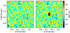 |
Fig. 1. Noise level obtained with ALMA observation of the nucleus of M31 in the CO(3–2) frequency range. The left panel displays the noise level achieved for Δv = 1000 km/s. The beam is presented in the lower left corner. In the right panel, the 2 mJy CO(1–0) signal expected by Chang et al. (2007), assuming R13 = 1.8, is superimposed on the noise map. |
3. Upper limits
Table 1 summarises the 3σ upper limits we achieved on the observed line intensities, together with the beam, integration time tint, and their observed frequencies, and Table 2 lists the 3σ upper limits on the continuum fluxes. Similarly, Figs. 2 and 3 illustrate the upper limits we reached with the measurements described in the previous section. In the following, we discuss the significance of these three types of upper limits on the molecular gas lines, the radio recombination line, and the continuum.
Different line observations (3σ upper limits).
Different continuum observations (3σ upper limits).
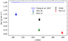 |
Fig. 2. Upper limits (3σ) on the line fluxes. The tick positions correspond to the 3σ upper values. The CO (H30α) line measurements are displayed in blue, green, and red (black). The prediction of Chang et al. (2007) is displayed with the horizontal blue line. |
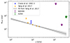 |
Fig. 3. Upper limits on the continuum flux. The blue and orange points correspond to the measurements of Crane et al. (1992, 1993), and Yang et al. (2017). The arrows correspond to the upper limits. The ticks correspond to the 3σ upper limit values. The line and associated error bars correspond to the fit discussed in Yang et al. (2017). |
3.1. Molecular gas
To derive upper limits on the total H2 mass, we computed the intrinsic CO luminosity with the velocity-integrated transition line flux FCO(J → J − 1)( ∝ SΔV) and calculated

where νrest is the rest CO line frequency, and DL is the luminosity distance (Solomon et al. 1997). We considered a luminosity distance of 0.78 Mpc for M31 (e.g. Stanek & Garnavich 1998). We then derived the total molecular gas mass including a correction of 36% for interstellar helium using

where the mass-to-light ratio αCO denotes the CO(1–0) conversion factor for the luminosity to the molecular gas mass, and  is the CO line ratio. Tacconi et al. (2018) assumed R12 ∼ 1.16 − 1.3 and R13 ∼ 1.8 for star formation main-sequence galaxies. The so-called CO-ladder ratios strongly depend on the column density and on the gas temperature (Combes et al. 1999; Weiss et al. 2007). Given the uncertainties here, we consider in the following standard values R12 ∼ 1.3 and R13 ∼ 1.8. For αCO, given the absence of gas, we assumed a Galactic value αCO = 4.36 M⊙/(K km s−1 pc2), which includes the usual correction to account for helium (e.g. Solomon et al. 1987; Genzel et al. 2010b; Bolatto et al. 2013). Again, we might consider that the gas in the central part is expected to have a high metallicity. However, various works (e.g. Bolatto et al. 2011; Genzel et al. 2012) that argued for a lower αCO for high-metallicity gas were based on actively star-forming galaxies. Alternatively, it is difficult to argue for a higher αCO, as expected in low-metallicity regions such as the outskirts of galaxies. Hence, upper values derived on the molecular gas are provided for the sake of discussion and for a comparison with standard MW values. As further discussed in Sect. 4, it is possible that the molecular gas in this region is CO-dark due to special physical conditions. The 3σ upper limits on the molecular mass derived from our measurements are provided in Table 3. The strongest constraint can be derived from the ALMA observations in CO(3–2). We can thus exclude that there are more than 195 M⊙ of molecular hydrogen within 1 pc of the nucleus, assuming standard MW-like conditions. This value is lower by a factor 50 than the mass of gas that was expected in the Chang et al. (2007) modelling.
Upper limits (3σ) on the intrinsic CO luminosity and on the molecular hydrogen mass.
3.2. Hydrogen recombination line
In Table 4, we summarise our results given our initial assumptions scaled from the previous observations of the H30α recombination line detected in the MW for SgrA* by Murchikova et al. (2019). The Bondi radius scales with the black hole mass RB = 2GM•/cs2 (where cs is the sound speed of the gas): The Bondi radius is thus a priori 35 times larger around the black hole of M31 than for SgrA* for a given sound speed
Comparison between the observed MW (Murchikova et al. 2019) and the expected ionised gas disc of M31, based on their relative black hole masses M• and distances D.
Relying on Baganoff et al. (2003), who estimated cs = 550 km s−1, we found a typical size of 4.2 pc, which is well sampled by our observations (0.3″or a resolution of 1.1 pc).
In addition, the line width ΔV traces the Keplerian velocity around the black hole and scales as  . Hence, given the previous assumption on the sound speed, we expect the same line width VH30α|M31 for M31 as for the MW,
Because of the similarities between the two nuclei, namely, their low Eddington ratios λEdd = L/LEdd of 2–4 × 10⁻⁹ and their radiatively inefficient accretion flow (RIAF), it is likely that they both possess a rotating ionised disc in their nuclei at a fraction of their Bondi radius. We thus know
The accretion rates are proportional to their respective BH masses. This corresponds to a typical (2D) accretion rate at the Bondi radius,
where μ is the ionised gas surface density. This means that we can assume the same plasma characteristics for the accretion around M31* and SgrA* (i.e. μ, cs, and the plane thickness h), and the accretion rate is 35 times higher for M31*,
![$$ \begin{aligned} \dot{M}_B|_{M31} = \left[ \dfrac{M_\bullet |_{M31}}{M_\bullet |_{MMW}} \right] \times \dot{M}_B|_{MW} = 35 \times \dot{M}_B|_{MW}. \end{aligned} $$](/articles/aa/full_html/2025/01/aa47597-23/aa47597-23-eq15.gif)
Last, the expected integrated signal can be written as
where ϵH30α is the emissivity of H30α (Storey & Hummer 1995), which varies weakly with the density. Assuming simple scaling relations, we find
![$$ \begin{aligned} S \Delta V_{H30\alpha }|_{M31}&= \left[\dfrac{D_{MW}}{D_{M31}}\right]^2 \left[ \dfrac{M_\bullet |_{M31}}{M_\bullet |_{MMW}}\right]^2 \times S \Delta V_{H30\alpha }|_{MW}\end{aligned} $$](/articles/aa/full_html/2025/01/aa47597-23/aa47597-23-eq17.gif)

The expected ionised gas signal in M31 is eight times lower than in the MW. The 3σ upper limit obtained here is 0.07 × the MW results. Therefore, our upper limit is twice below what was expected. This means that the nucleus of M31 has less ionised gas than SgrA* in proportion.
3.3. Continuum flux
Our upper limits are compatible with the synchrotron power-law emission that was derived from lower-frequency measurements (Crane et al. 1992, 1993; Yang et al. 2017). Given the absence of gas in the nucleus, no dust emission is expected.
4. Discussion and conclusions
The ALMA observations present an unprecedented sensitivity for cold molecular gas and further exclude its presence next to the black hole. The modelling proposed by Chang et al. (2007) predicted 104 M⊙ of molecular gas H2 based on CO(1–0), while our ALMA upper limit (195 M⊙ of H2 derived from CO(3–2) measurements) is 50 times lower and excludes this modelling at a level of 150σ. While the principle of gas replenishment through stellar winds from red giants in the eccentric disc is reasonable, some details are probable incorrect. In addition to the small rotation pattern requirement that seems compatible with modern estimates (e.g. Lockhart et al. 2018), the values used for the stellar wind mass-loss rates lie on the upper side of the expected range and might be overestimated by a factor larger than 50 (E. Josselin, priv. comm.). The modelling might still account for the formation of the blue nuclear cluster next to P3 (Lauer et al. 2012), but the timescale for reconstituting a gas reservoir would then be longer than expected. Alternatively, Demarque & Virani (2007) also discussed that the central blue nucleus might be composed of an old stellar population of evolved blue horizontal branch stars and of merger products, which would invalidate the need of gas inflow to form it. We highlight the difference with the configuration of the nuclear cluster hosted next to SgrA*, which hosts, within 1 pc, 96% of old (< 1 Gyr) stars (Genzel et al. 2010a), but also the so-called S-star cluster (Eckart & Genzel 1996), where 177 O, WR, and B stars were spectroscopically identified. A central neutral gas cavity of 1.5 pc is observed and has probably been produced by stellar winds from the young massive stars. Inside a radius of 200 pc, the central molecular zone hosts a dense and massive medium containing 5 − 10 × 107 M⊙ of gas (Morris & Serabyn 1996). This gas then inflows through the mini-spiral streamers towards the circumnuclear disc at an apparent rate of 10−3 M⊙ yr−1 (Genzel et al. 1994). The observed molecular gas of this disc of a few parsec is clumpy, and its molecular mass is estimated to be about 105 − 106 M⊙ if the gas is stable and virialised (Montero-Castaño et al. 2009), even though the weak ratio of the far-IR to millimetre dust continuum suggests that it might be a less massive transient disc of 104 M⊙ (Mezger et al. 1996). With the assumption of virial equilibrium, we estimated for the equivalent of the central molecular zone in Andromeda a total H2 mass of about (8.4 ± 0.4)×104 M⊙ within 250 pc (Dassa-Terrier et al. 2019). We showed that the molecular H2 mass hosted by the M31 CND is lower than 195 M⊙.
Relying on simple scaling relations based on the Murchikova et al. (2019) detection of the H30α recombination line next to SgrA*, we tentatively searched this line next to M31* with deep NOEMA observations. We excluded it at a 6σ level. In the optical, Menezes et al. (2013) discovered an eccentric Hα-emitting disc in the nucleus of M31, with a radius of 0.7″. This optical recombination line traces some gas next to the nucleus. The authors estimated that this gas disc with a radius of 2.7 pc has a luminosity of LHα = (8.7 ± 1)×102 L⊙. This luminosity corresponds to a recombination rate of 1048 photons per second. The possible mechanisms that might have ionised this gas are discussed below. Following Jacoby et al. (1985), one typical planetary nebula emits 1.2 × 1045 photons per second, and we do not expect more than a few planetary nebulae in this region (e.g. Pastorello et al. 2013). The youngest stars present in this region belongs to the A0-star cluster (4200 M⊙) next to the black hole in P3 (Bender et al. 2005). Their typical temperature 10 000 K (Drilling & Landolt 2000) excludes any significant number of ionising photons. Assuming a blackbody emission, such an A0-star with a typical mass of 2.5 M⊙ cannot produce more that 1.2 × 1038 recombinations per second, corresponding to a grand total of 2 × 1041 recombinations per second. We can thus exclude that stellar objects contribute to the ionisation of this central gas.
On 6th January 2006, Li et al. (2011) observed a murmur of M31* at a level of 4.3 × 1037 erg s−1 in the frequency range 0.5 − 8 keV, corresponding to a minimum of 2 × 1048 recombinations per second. The previous relic activity of the central engine might well explain the excitation of this inner Hα disc. An episodic activity of the black hole is also supported by the work of Zhang et al. (2019), which was based on X-ray gas. The authors concluded that only an AGN episode half a million years ago could account for their observed line ratios. In addition, on probably different timescales, Pshirkov et al. (2016) also discussed signs of recent AGN activity found in possible Fermi bubbles, while Bogdán & Gilfanov (2008) detected the possible relic of a previous outflow. Recurrent bursts from the central engine might account for the whole picture. It is therefore possible that the CO has been destroyed, as proposed by Bisbas et al. (2015), by the black hole activity traced in the X-rays. Moreover, Jimenez et al. (2007) showed that the irradiation by an AGN can modify the atmosphere of red giant stars. While the level of X-ray activity of SgrA* is comparable with the activity observed for M31* (e.g. Inayoshi et al. 2020), its numerous flares are monitored at the present epoch (Mossoux et al. 2020) and also in the past 100 years, as observed by reflection (Clavel et al. 2013). Three main scenarii have been considered to account for these flares: (1) stellar winds from massive stars such as IRS 13 E3 (e.g. Mościbrodzka et al. 2006); (2) accretion of a gas clump such as G2 (e.g. Gillessen et al. 2013; Czerny et al. 2013; Owen & Lin 2023); and (3) tidal disruption by an asteroid or solid body passing by (e.g. Zubovas et al. 2012). For M31, the absence of massive stars excludes the first scenario. Our results weaken the second scenario, as we were not able to detect any molecular cloud. The weak detection of Hα leaves the possibility of gas accretion from diffuse ionised gas. We finally cannot exclude the third scenario.
Our upper limits on the molecular H2 mass (195 M⊙ (3σ) based on ALMA CO(3 − 2) observations) and the detection of a weak Hα disc by Menezes et al. (2013) support the evidence of previous activity of the AGN (e.g. kinetic jet feedback), which might have significantly contributed to centrally quench this galaxy, as discussed by Huško et al. (2024).
Acknowledgments
This paper makes use of the following ALMA data: ADS/JAO.ALMA#2019.1.00711.S. ALMA is a partnership of ESO (representing its member states), NSF (USA) and NINS (Japan), together with NRC (Canada), MOST and ASIAA (Taiwan), and KASI (Republic of Korea), in cooperation with the Republic of Chile. The Joint ALMA Observatory is operated by ESO, AUI/NRAO and NAOJ. This work is based on observations carried out under project numbers W19BN and W01E with the IRAM NOEMA Interferometer. IRAM is supported by INSU/CNRS (France), MPG (Germany) and IGN (Spain). This work benefited from the support of the Action fédératrice ALMA-NOEMA of Paris Observatory, and in particular the workshop organised within this project by Raphaël Moreno and Philippe Salomé. This project also got from support from the Programme National Cosmologie et Galaxies. Special thanks go to Eric Josselin and Franck Delahaye for useful information on stellar populations. Last, we are most grateful to the anonymous referee for the very constructive comments that helped us to substantially improve the manuscript.
References
- Bacon, R., Emsellem, E., Combes, F., et al. 2001, A&A, 371, 409 [NASA ADS] [CrossRef] [EDP Sciences] [Google Scholar]
- Baganoff, F. K., Maeda, Y., Morris, M., et al. 2003, ApJ, 591, 891 [Google Scholar]
- Belfiore, F., Maiolino, R., & Bothwell, M. 2016, MNRAS, 455, 1218 [CrossRef] [Google Scholar]
- Bender, R., Kormendy, J., Bower, G., et al. 2005, ApJ, 631, 280 [NASA ADS] [CrossRef] [Google Scholar]
- Bisbas, T. G., Papadopoulos, P. P., & Viti, S. 2015, ApJ, 803, 37 [NASA ADS] [CrossRef] [Google Scholar]
- Bogdán, Á., & Gilfanov, M. 2008, MNRAS, 388, 56 [NASA ADS] [CrossRef] [Google Scholar]
- Bolatto, A. D., Leroy, A. K., Jameson, K., et al. 2011, ApJ, 741, 12 [CrossRef] [Google Scholar]
- Bolatto, A. D., Wolfire, M., & Leroy, A. K. 2013, ARA&A, 51, 207 [CrossRef] [Google Scholar]
- Chang, P., Murray-Clay, R., Chiang, E., & Quataert, E. 2007, ApJ, 668, 236 [NASA ADS] [CrossRef] [Google Scholar]
- Clavel, M., Terrier, R., Goldwurm, A., et al. 2013, A&A, 558, A32 [NASA ADS] [CrossRef] [EDP Sciences] [Google Scholar]
- Combes, F., Maoli, R., & Omont, A. 1999, A&A, 345, 369 [NASA ADS] [Google Scholar]
- Crane, P. C., Dickel, J. R., & Cowan, J. J. 1992, ApJ, 390, L9 [NASA ADS] [CrossRef] [Google Scholar]
- Crane, P. C., Cowan, J. J., Dickel, J. R., & Roberts, D. A. 1993, ApJ, 417, L61 [NASA ADS] [CrossRef] [Google Scholar]
- Czerny, B., Kunneriath, D., Karas, V., & Das, T. K. 2013, A&A, 555, A97 [NASA ADS] [CrossRef] [EDP Sciences] [Google Scholar]
- Dassa-Terrier, J., Melchior, A.-L., & Combes, F. 2019, A&A, 625, A148 [NASA ADS] [CrossRef] [EDP Sciences] [Google Scholar]
- Demarque, P., & Virani, S. 2007, A&A, 461, 651 [NASA ADS] [CrossRef] [EDP Sciences] [Google Scholar]
- Dong, H., Li, Z., Wang, Q. D., et al. 2015, MNRAS, 451, 4126 [Google Scholar]
- Dong, H., Olsen, K., Lauer, T., et al. 2018, MNRAS, 478, 5379 [Google Scholar]
- Dosaj, A., Garcia, M., Forman, W., et al. 2002, ASP Conf. Ser., 262, 147 [Google Scholar]
- Drilling, J. S., & Landolt, A. U. 2000, in Allen’s Astrophysical Quantities, ed. A. N. Cox, 381 [Google Scholar]
- Eckart, A., & Genzel, R. 1996, Nature, 383, 415 [NASA ADS] [CrossRef] [Google Scholar]
- Esin, A. A. 1997, ApJ, 482, 400 [NASA ADS] [CrossRef] [Google Scholar]
- Feng, L., Li, Z.-Y., Su, M., Tam, P.-H. T., & Chen, Y. 2019, Res. Astron. Astrophys., 19, 046 [Google Scholar]
- Garcia, M. R., Hextall, R., Baganoff, F. K., et al. 2010, ApJ, 710, 755 [NASA ADS] [CrossRef] [Google Scholar]
- Genzel, R., Hollenbach, D., & Townes, C. H. 1994, Rep. Prog. Phys., 57, 417 [NASA ADS] [CrossRef] [Google Scholar]
- Genzel, R., Eisenhauer, F., & Gillessen, S. 2010a, Rev. Mod. Phys., 82, 3121 [Google Scholar]
- Genzel, R., Tacconi, L. J., Gracia-Carpio, J., et al. 2010b, MNRAS, 407, 2091 [NASA ADS] [CrossRef] [Google Scholar]
- Genzel, R., Tacconi, L. J., Combes, F., et al. 2012, ApJ, 746, 69 [Google Scholar]
- Gillessen, S., Genzel, R., Fritz, T. K., et al. 2013, ApJ, 763, 78 [NASA ADS] [CrossRef] [Google Scholar]
- Heckman, T. M. 1996, ASP Conf. Ser., 103, 241 [NASA ADS] [Google Scholar]
- Heckman, T. M., & Best, P. N. 2014, ARA&A, 52, 589 [Google Scholar]
- Hopkins, P. F., & Quataert, E. 2010a, MNRAS, 407, 1529 [Google Scholar]
- Hopkins, P. F., & Quataert, E. 2010b, MNRAS, 405, L41 [NASA ADS] [Google Scholar]
- Huško, F., Lacey, C. G., Schaye, J., Nobels, F. S. J., & Schaller, M. 2024, MNRAS, 527, 5988 [Google Scholar]
- Inayoshi, K., Ostriker, J. P., Haiman, Z., & Kuiper, R. 2018, MNRAS, 476, 1412 [Google Scholar]
- Inayoshi, K., Visbal, E., & Haiman, Z. 2020, ARA&A, 58, 27 [NASA ADS] [CrossRef] [Google Scholar]
- Jacoby, G. H., Ford, H., & Ciardullo, R. 1985, ApJ, 290, 136 [NASA ADS] [CrossRef] [Google Scholar]
- Jimenez, R., da Silva, J. P., Oh, S. P., Jørgensen, U. G., & Merritt, D. 2007, ApJ, 661, 203 [NASA ADS] [CrossRef] [Google Scholar]
- Lauer, T. R., Bender, R., Kormendy, J., Rosenfield, P., & Green, R. F. 2012, ApJ, 745, 121 [NASA ADS] [CrossRef] [Google Scholar]
- Leahy, D. A., Bianchi, L., & Postma, J. E. 2018, AJ, 156, 269 [CrossRef] [Google Scholar]
- Leahy, D., Seminoff, N., & Leahy, C. 2022, AJ, 163, 138 [NASA ADS] [CrossRef] [Google Scholar]
- Leigh, N. W. C., Antonini, F., Stone, N. C., Shara, M. M., & Merritt, D. 2016, MNRAS, 463, 1605 [NASA ADS] [CrossRef] [Google Scholar]
- Li, Z., Garcia, M. R., Forman, W. R., et al. 2011, ApJ, 728, L10 [NASA ADS] [CrossRef] [Google Scholar]
- Lockhart, K. E., Lu, J. R., Peiris, H. V., et al. 2018, ApJ, 854, 121 [NASA ADS] [CrossRef] [Google Scholar]
- Madigan, A.-M., Halle, A., Moody, M., et al. 2018, ApJ, 853, 141 [CrossRef] [Google Scholar]
- McCourt, M., Oh, S. P., O’Leary, R., & Madigan, A.-M. 2018, MNRAS, 473, 5407 [Google Scholar]
- Melchior, A. L., & Combes, F. 2011, A&A, 536, A52 [NASA ADS] [CrossRef] [EDP Sciences] [Google Scholar]
- Melchior, A. L., & Combes, F. 2013, A&A, 549, A27 [NASA ADS] [CrossRef] [EDP Sciences] [Google Scholar]
- Melchior, A.-L., & Combes, F. 2016, A&A, 585, A44 [NASA ADS] [CrossRef] [EDP Sciences] [Google Scholar]
- Melchior, A.-L., & Combes, F. 2017, A&A, 607, L7 [NASA ADS] [CrossRef] [EDP Sciences] [Google Scholar]
- Melchior, A. L., Viallefond, F., Guélin, M., & Neininger, N. 2000, MNRAS, 312, L29 [NASA ADS] [CrossRef] [Google Scholar]
- Menezes, R. B., Steiner, J. E., & Ricci, T. V. 2013, ApJ, 762, L29 [NASA ADS] [CrossRef] [Google Scholar]
- Mezger, P. G., Duschl, W. J., & Zylka, R. 1996, A&ARv, 7, 289 [NASA ADS] [CrossRef] [Google Scholar]
- Montero-Castaño, M., Herrnstein, R. M., & Ho, P. T. P. 2009, ApJ, 695, 1477 [CrossRef] [Google Scholar]
- Morris, M., & Serabyn, E. 1996, ARA&A, 34, 645 [Google Scholar]
- Mościbrodzka, M., Das, T. K., & Czerny, B. 2006, MNRAS, 370, 219 [CrossRef] [Google Scholar]
- Mossoux, E., Finociety, B., Beckers, J. M., & Vincent, F. H. 2020, A&A, 636, A25 [NASA ADS] [CrossRef] [EDP Sciences] [Google Scholar]
- Müller, A., & Camenzind, M. 2004, A&A, 413, 861 [NASA ADS] [CrossRef] [EDP Sciences] [Google Scholar]
- Murchikova, E. M., Phinney, E. S., Pancoast, A., & Blandford, R. D. 2019, Nature, 570, 83 [NASA ADS] [CrossRef] [Google Scholar]
- Murchikova, L., White, C. J., & Ressler, S. M. 2022, ApJ, 932, L21 [NASA ADS] [CrossRef] [Google Scholar]
- Neumayer, N., Seth, A., & Böker, T. 2020, A&ARv, 28, 4 [Google Scholar]
- Owen, J. E., & Lin, D. N. C. 2023, MNRAS, 519, 397 [Google Scholar]
- Pastorello, N., Sarzi, M., Cappellari, M., et al. 2013, MNRAS, 430, 1219 [Google Scholar]
- Paumard, T., Genzel, R., Martins, F., et al. 2006, ApJ, 643, 1011 [NASA ADS] [CrossRef] [Google Scholar]
- Pshirkov, M. S., Vasiliev, V. V., & Postnov, K. A. 2016, MNRAS, 459, L76 [Google Scholar]
- Rossa, J., van der Marel, R. P., Böker, T., et al. 2006, AJ, 132, 1074 [NASA ADS] [CrossRef] [Google Scholar]
- Seth, A. C., Dalcanton, J. J., Hodge, P. W., & Debattista, V. P. 2006, AJ, 132, 2539 [NASA ADS] [CrossRef] [Google Scholar]
- Solomon, P. M., Rivolo, A. R., Barrett, J., & Yahil, A. 1987, ApJ, 319, 730 [Google Scholar]
- Solomon, P. M., Downes, D., Radford, S. J. E., & Barrett, J. W. 1997, ApJ, 478, 144 [NASA ADS] [CrossRef] [Google Scholar]
- Stanek, K. Z., & Garnavich, P. M. 1998, ApJ, 503, L131 [Google Scholar]
- Storey, P. J., & Hummer, D. G. 1995, MNRAS, 272, 41 [NASA ADS] [CrossRef] [Google Scholar]
- Tacconi, L. J., Genzel, R., Saintonge, A., et al. 2018, ApJ, 853, 179 [Google Scholar]
- Tremaine, S. 1995, AJ, 110, 628 [NASA ADS] [CrossRef] [Google Scholar]
- Weiss, A., Downes, D., Walter, F., & Henkel, C. 2007, ASP Conf. Ser., 375, 25 [NASA ADS] [Google Scholar]
- Yang, Y., Li, Z., Sjouwerman, L. O., Yuan, F., & Shen, Z.-Q. 2017, ApJ, 845, 140 [CrossRef] [Google Scholar]
- Zhang, S., Wang, Q. D., Foster, A. R., et al. 2019, ApJ, 885, 157 [CrossRef] [Google Scholar]
- Zubovas, K., Nayakshin, S., & Markoff, S. 2012, MNRAS, 421, 1315 [NASA ADS] [CrossRef] [Google Scholar]
All Tables
Upper limits (3σ) on the intrinsic CO luminosity and on the molecular hydrogen mass.
Comparison between the observed MW (Murchikova et al. 2019) and the expected ionised gas disc of M31, based on their relative black hole masses M• and distances D.
All Figures
|
Fig. 1. Noise level obtained with ALMA observation of the nucleus of M31 in the CO(3–2) frequency range. The left panel displays the noise level achieved for Δv = 1000 km/s. The beam is presented in the lower left corner. In the right panel, the 2 mJy CO(1–0) signal expected by Chang et al. (2007), assuming R13 = 1.8, is superimposed on the noise map. |
| In the text | |
|
Fig. 2. Upper limits (3σ) on the line fluxes. The tick positions correspond to the 3σ upper values. The CO (H30α) line measurements are displayed in blue, green, and red (black). The prediction of Chang et al. (2007) is displayed with the horizontal blue line. |
| In the text | |
|
Fig. 3. Upper limits on the continuum flux. The blue and orange points correspond to the measurements of Crane et al. (1992, 1993), and Yang et al. (2017). The arrows correspond to the upper limits. The ticks correspond to the 3σ upper limit values. The line and associated error bars correspond to the fit discussed in Yang et al. (2017). |
| In the text | |
Current usage metrics show cumulative count of Article Views (full-text article views including HTML views, PDF and ePub downloads, according to the available data) and Abstracts Views on Vision4Press platform.
Data correspond to usage on the plateform after 2015. The current usage metrics is available 48-96 hours after online publication and is updated daily on week days.
Initial download of the metrics may take a while.