| Issue |
A&A
Volume 692, December 2024
|
|
|---|---|---|
| Article Number | A196 | |
| Number of page(s) | 16 | |
| Section | Stellar structure and evolution | |
| DOI | https://doi.org/10.1051/0004-6361/202452300 | |
| Published online | 16 December 2024 | |
Analytic insight into the physics of the standing accretion shock instability
I. Shock instability in a non-rotating stellar core
Université Paris-Saclay, Université Paris Cité, CEA, CNRS, AIM, 91191 Gif-sur-Yvette, France
⋆ Corresponding author; This email address is being protected from spambots. You need JavaScript enabled to view it.
Received:
18
September
2024
Accepted:
23
October
2024
Abstract
Context. During the core collapse of a massive star, and immediately before its supernova explosion, there is amplification of asymmetric motions by the standing accretion shock instability (SASI). This imprints a frequency signature on the neutrino flux and the gravitational waves that carries direct information about the explosion process.
Aims. The physical interpretation of this multi-messenger signature requires a detailed understanding of the instability mechanism.
Methods. We carried out a perturbative analysis to characterise the properties of SASI and assess the effect of the region of neutronization above the surface of the proto-neutron star. We compared the eigenfrequencies of the most unstable modes to those obtained in an adiabatic approximation where neutrino interactions are neglected above the neutrinosphere. We solved the differential system analytically using a Wronskian method and approximated it asymptotically for a large shock radius.
Results. The oscillation period of SASI is well fitted with a simple analytic function of the shock radius, the radius of maximum deceleration, and the mass of the proto-neutron star. The oscillation period is weakly dependent on the parameterised cooling function, but this latter does affects the SASI growth rate. We describe the general properties of SASI eigenmodes using an adiabatic model. In this approximation, the eigenvalue problem is formulated as a self-forced oscillator. The forcing agent is the radial advection of baroclinic vorticity perturbations and entropy perturbations produced by the shock oscillation. We reduced the differential system defining the eigenfrequencies to a single integral equation. Its analytical approximation sheds light on the radially extended character of the region of advective-acoustic coupling. The simplicity of this adiabatic formalism opens new perspectives for the investigation of the effect of stellar rotation and non-adiabatic processes on SASI.
Key words: hydrodynamics / instabilities / neutrinos / shock waves / stars: neutron / supernovae: general
© The Authors 2024
 Open Access article, published by EDP Sciences, under the terms of the Creative Commons Attribution License (https://creativecommons.org/licenses/by/4.0), which permits unrestricted use, distribution, and reproduction in any medium, provided the original work is properly cited.
This article is published in open access under the Subscribe to Open model. This email address is being protected from spambots. You need JavaScript enabled to view it. to support open access publication.
1. Introduction
The explosive death of massive stars is sensitive to the development of hydrodynamical instabilities, which break the spherical symmetry of the stellar core, affect the efficiency of neutrino energy absorption, and generate turbulence (Müller 2020; Janka et al. 2016; Burrows & Vartanyan 2021). A spherically symmetric scenario based on radial motions seems possible only for the lightest progenitors (Kitaura et al. 2006; Stockinger et al. 2020). Asymmetric motions contribute to the kick and spin of the neutron star (Müller et al. 2019; Janka 2017), the emission of gravitational waves (Kotake & Kuroda 2017), and a modulation of neutrino emission (Müller 2019b; Tamborra & Murase 2019). Drago et al. (2023) considered the correlation of instability signatures in the gravitational waves and neutrino signals in order to improve the efficiency with which we can detect gravitational waves from nearby supernovae. Ultimately, the information encoded in the gravitational waves and neutrino signals can be used to recover the properties of the dying star and its explosion mechanism (Powell & Müller 2022). The computational cost of 3D numerical simulations precludes systematic coverage of the large parameter space describing the initial conditions of stellar core collapse. Understanding the underlying mechanism of hydrodynamical instabilities is essential to extrapolating the results of sparse numerical simulations, evaluating the impact of additional physical ingredients, and designing effective prescriptions for parametric studies (Müller 2019a).
Among the hydrodynamical instabilities at work during the phase of stalled accretion shock, the standing accretion shock instability (SASI; Blondin et al. 2003) is able to introduce coherent transverse motions with a large angular scale, growing over a timescale related to the advection time from the shock to the neutron star surface. The mechanism of SASI has been described as an advective-acoustic cycle between the shock and the vicinity of the proto-neutron star (Foglizzo et al. 2007; Fernández & Thompson 2009b; Scheck et al. 2008). Our analytical understanding of SASI eigenfrequencies in the WKB approximation is however restricted to the limit of a large shock radius for high-frequency overtones (Foglizzo et al. 2007), while the lowest-frequency fundamental mode is often the most unstable. A fully analytic solution including the fundamental mode was obtained only in a very idealised model, where the stationary flow is plane parallel and uniform except in a compact region of deceleration that mimics the vicinity of the neutron star (Foglizzo 2009) (hereafter F09). This toy model neglected the flow gradients that are extended all the way from the shock to the neutron star and the non-adiabatic character of the neutrino processes taking place in the vicinity of the neutron star. Despite these limitations, this model illustrated the interplay of the advective-acoustic and the purely acoustic cycles, and the expected phase mixing taking place at high frequency. The model was used by Guilet & Foglizzo (2012) to interpret the frequency spacing of the eigenspectrum in the framework of the advective-acoustic mechanism rather than a purely acoustic process. The physical understanding of SASI led Müller & Janka (2014) to define an empirical formula for the SASI oscillation period in order to interpret the modulation of the neutrino signal. Directly proportional to an approximation of the advection time from the shock to the neutron star surface, it was tested on a 2D numerical simulation of the collapse of a 25 M⊙ progenitor. However, whether or not it can be generalised for other progenitors, as proposed by Müller (2019b), remains unclear.
The aim of the present study is to improve our understanding of the fundamental mode of SASI in spherical geometry in order to better identify the physical parameters governing its oscillation frequency. Simple cooling functions mimicking neutrino emission are used to assess the role of the cooling region. An adiabatic approximation is also used to assess the role of the advective-acoustic coupling in the radially extended region between the shock and the proto-neutron star. The adiabatic approximation is motivated by the adiabatic simulations of Blondin & Mezzacappa (2007) and by the shallow-water experiment (Foglizzo et al. 2012, 2015), which both suggest that several properties of SASI may be understood using adiabatic equations. Dunham et al. (2024) have also used the adiabatic approximation to analyse the impact of general relativistic corrections on SASI eigenfrequencies.
The set of differential equations defining the eigenfrequencies of spherical accretion are recalled in Sect. 2, with particular attention being paid to the radial extension of the non-adiabatic cooling layer and its impact on the oscillation period of SASI. The eigenfrequencies calculated in the adiabatic approximation are compared to those including neutrino losses in Sect. 3. The adiabatic model is formulated as a self-forced oscillator in Sect. 4, with eigenfrequencies defined by an integral equation. An analytic approximation of this equation is outlined and analysed in Sect. 5. Conclusions and perspectives are formulated in Sect. 6.
2. Stationary accretion with non-adiabatic cooling
2.1. Stationary flow
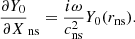
We use the same general framework as Blondin et al. (2003), Foglizzo et al. (2007), Blondin et al. (2017) to describe the phase where the accretion shock stalls at the radius rsh. Neutrino absorption is neglected and neutrino emission near the proto-neutron star radius rns is idealised with a cooling function of the density ρ and pressure p:
 (1)
(1)
The collapsing stellar core immediately after bounce is modelled as a perfect gas with an adiabatic index of γ = 4/3, dominated by the degeneracy pressure of relativistic electrons. The gravitational potential Φ ≡ −GMns/r is assumed to be dominated by the mass Mns of the proto-neutron star in the Newtonian approximation for simplicity. We neglect the self-gravity of the accreting gas and the increase in Mns with time. The dimensionless measure of the entropy S is defined as
 (2)
(2)
The stationary flow is described by the mass conservation, the entropy equation, and the Euler equation:
 (3)
(3)
 (4)
(4)
 (5)
(5)
where c ≡ (γp/ρ)1/2 is the sound speed and v < 0 the radial velocity. The geometrical parameter g = 2 accounting for the spherical geometry is noted as a parameter in this section and Sect. 3 to keep track of its impact on the equations in the spirit of Walk et al. (2023). The subscript ‘sh’ in Eq. (3) refers to quantities immediately below the shock, and the subscript ‘1’ refers to pre-shock quantities. The jump conditions at the shock follow from the conservation of mass flux and momentum flux, taking into account the energy lost across the shock through nuclear dissociation. This latter is modelled as in Fernández & Thompson (2009b), Fernández et al. (2014) by the parameter ε, which is a measure of the energy loss Δedisso per unit of mass in units of the pre-shock kinetic energy density v12/2 as in Huete et al. (2018):
 (6)
(6)
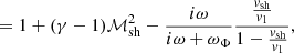
The effect of ε on the post-shock Mach number ℳsh and the Rankine-Hugoniot conditions is described in Appendix A, following Eqs. (A.4)–(A.6) of Foglizzo et al. (2006). The pre-shock deceleration effect of pressure is neglected, with v12 ∼ 2GMns/rsh. Defining the Mach number ℳ ≡|v|/c as positive, we assume a strong adiabatic shock ℳ1 ≫ 1 in the numerical calculations of this section.
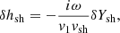
The adiabatic compression of the post-shock flow by the gravitational potential Φ produces an inward increase in the enthalpy c2/(γ − 1) and thus an increase in the gas temperature T ∝ c2 according to the Bernoulli Eq. (5). In our model of stationary accretion, the temperature profile displays a maximum at a radius denoted rpeak, where the energy losses by neutrino emission balance the adiabatic heating due to the gravitational compression. The width of the cooling layer depends a priori on the parameters (α, β) of the cooling function ℒ, the mass accretion rate, and the geometry. With α = 3/2 and β = 5/2, Walk et al. (2023) noted that both the radius rpeak ∼ 1.2rns of maximum temperature and the typical width Δrpeak ∼ 1.5rns of the temperature profile measured at half maximum seemed surprisingly independent of both the mass-accretion rate and the shock radius, and also seemed independent of the geometry. Closer inspection confirms that the location of rpeak varies by less than 1% between the cylindrical and spherical geometries, and varies by less than 0.5% with rsh for rsh/rns > 3.
Figure 1 compares rpeak to the radius of maximum deceleration denoted r∇, with r∇ < rpeak over a large range of parameters (α, β), except for when β approaches unity. Noting that r∇ = rns for α < β (Foglizzo et al. 2007), Fig. 1 indicates that rpeak/r∇ ∼ 1.2 for (α, β) = (3/2, 5/2), and rpeak/r∇ ∼ 1.0 for (α, β) = (6, 1). In Sect. 2.2, the parameters (α, β) are varied continuously from (3/2, 5/2) to (6, 1) and from (3/2, 5/2) to (5, 6) in order to evaluate their impact on SASI properties.
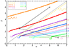 |
Fig. 1. Ratios rpeak/rns (thick solid lines) and r∇/rns (thin dotted lines) depending on the coefficients (α, β) that define the cooling function in Eq. (1). The contour lines are calculated for γ = 4/3 in spherical geometry, with rsh/rns = 10, without dissociation (ε = 0). The values of rpeak/rns and r∇/rns are indicated with the same colour code. The cooling parameters (α, β) = (3/2, 5/2), (6, 1) and (5, 6) used in Fig. 3 are indicated with crosses for reference and are connected by grey lines. The black dotted line marks the threshold β = α above which the advection time from rpeak to rns is finite and r∇ = rns. |
2.2. Perturbed flow
The perturbations of the stationary flow are characterised by the wavenumbers ℓ, m of spherical harmonics and a complex eigenfrequency ω. The eigenfrequency is independent of the azimuthal wavenumber |m|≤ℓ as established in Foglizzo et al. (2007). We use the same physical variables as in Foglizzo et al. (2006) guided by analytical simplicity, namely the perturbation of the Bernoulli constant δf, the perturbed mass flux δh, and the perturbed dimensionless entropy δS. The perturbation δK is a combination of perturbed entropy δS and the quantity δw⊥ defined from the radial component of the curl of the vorticity perturbation δw ≡ ∇ × δv:
 (7)
(7)
 (8)
(8)
 (9)
(9)
 (10)
(10)
![Mathematical equation: $$ \begin{aligned}&= {1\over \sin \theta } \left[{\partial \over \partial \theta }(\delta { w}_\varphi \sin \theta )-im \delta { w}_\theta \right], \end{aligned} $$](/articles/aa/full_html/2024/12/aa52300-24/aa52300-24-eq11.gif) (11)
(11)
 (12)
(12)
We introduce the quantity δA, which is defined as the divergence of the ortho-radial velocity δv⊥ ≡ (0, δvθ, δvφ):
 (13)
(13)
![Mathematical equation: $$ \begin{aligned}&= {r\over \sin \theta } \left[{\partial \over \partial \theta }(\delta { v}_\theta \sin \theta )+im \delta { v}_\varphi \right]. \end{aligned} $$](/articles/aa/full_html/2024/12/aa52300-24/aa52300-24-eq14.gif) (14)
(14)
We establish in Appendix B that δA and δw⊥ are related to the perturbation δvr of the radial velocity as
 (15)
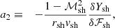
(15)
This equation invites us to interpret δA/ℓ(ℓ + 1) as the potential defining the compressible part of the perturbed velocity, and rδw⊥/ℓ(ℓ + 1) as the rotational contribution to the radial velocity perturbation. Using the transverse components of the Euler equation Eqs. (B.10), (B.11) in Appendix B with Eq. (12), we note that δA is related to δK and δf as
 (16)
(16)
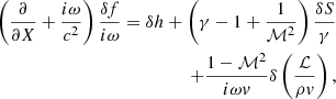
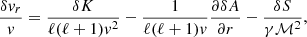
The differential system satisfied by (δA, δh, δS, δK) is as follows:
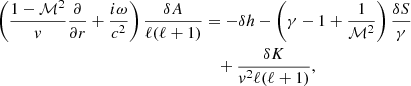 (17)
(17)
 (18)
(18)
 (19)
(19)
 (20)
(20)
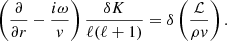
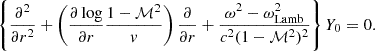
This system includes explicit non-adiabatic terms only in the Eqs. (19, 20) governing δS and δK. In Eq. (18), the Lamb frequency ωLamb associated with the spherical harmonic of order ℓ defines the turning point of non-radial acoustic waves:
 (21)
(21)
The boundary conditions at the shock are reformulated from Eqs. (28, 29, E.7, E.8) in Foglizzo et al. (2006) using Eq. (16):
 (22)
(22)
 (23)
(23)
 (24)
(24)
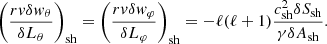
![Mathematical equation: $$ \begin{aligned} \delta K_{\rm sh}&= - \ell (\ell +1)\Delta \zeta {c^2_{\rm sh}\over \gamma } \left[\nabla S\right]^\mathrm{sh}_{1} \ , \end{aligned} $$](/articles/aa/full_html/2024/12/aa52300-24/aa52300-24-eq25.gif) (25)
(25)
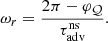
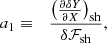
where Δζ and Δv ≡ −iωΔζ are the shock displacement and velocity, respectively. The reference frequency ωΦ in Eq. (24) is defined as
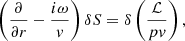
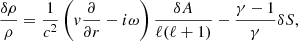
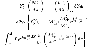
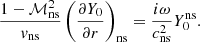
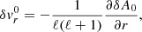
![Mathematical equation: $$ \begin{aligned} {\omega _\Phi r_{\rm sh}\over |{ v}_{\rm sh}|} \equiv {1\over 2}{{ v}_1\over {{ v}_{\rm sh}}} { {2r_{\rm sh}\over { v}_1^2}{\mathrm{d}\Phi \over \mathrm{d} r} -4{{{ v}_{\rm sh}}\over { v}_1} \over 1-{{{ v}_{\rm sh}}\over { v}_{1}} } + {{{{ v}_{\rm sh}}\over { v}_1}\over \gamma \mathcal{M}_{\rm sh}^2} { r_{\rm sh}\left[\nabla S\right]^\mathrm{sh}_{1} \over \left(1-{{{ v}_{\rm sh}}\over { v}_{1}}\right)^2 }, \end{aligned} $$](/articles/aa/full_html/2024/12/aa52300-24/aa52300-24-eq26.gif) (26)
(26)
where ωΦ defines the threshold frequency separating the regime (ω ≪ ωΦ) – where the phase of δSsh is opposed to that of Δζ – from the regime (ω ≫ ωΦ), where the phase of δSsh is set by that of Δv.
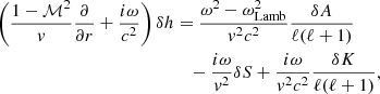
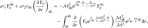
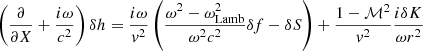
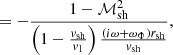
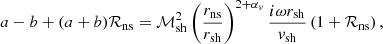
The first two differential equations (17)–(18) are transformed into the following second-order differential equation:
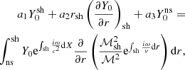
![Mathematical equation: $$ \begin{aligned} \left[\left( {1-\mathcal{M}^2\over { v}} {\partial \over \partial r}+{i\omega \over c^2}\right)^2 + {\omega ^2-\omega _{\rm Lamb}^2\over { v}^2c^2}\right]\delta A = \nonumber \\ {\partial \over \partial r} {r\delta { w}_\perp \over { v}} -\ell (\ell +1) {\gamma -1\over \gamma } \delta \left( {\mathcal{L}\over p { v}} \right) . \end{aligned} $$](/articles/aa/full_html/2024/12/aa52300-24/aa52300-24-eq27.gif) (27)
(27)
We recognise an acoustic oscillator modified by advection on the left-hand side of Eq. (27), with a forcing on the right-hand side driven by vorticity perturbations and by the perturbation of neutrino cooling. Interestingly, part of this forcing can be studied analytically in the adiabatic approximation defined in Sect. 3.
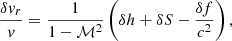
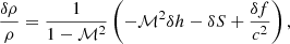
The variables δvr, δρ, δc, and δp are deduced from δA, δh, δS, and δK using Eqs. (B.4)–(B.7), as detailed in Appendix B. In particular, using Eq. (B.4) to express the lower boundary condition δvr(rns) = 0, leads to
 (28)
(28)
With a vanishing sound speed cns = 0 resulting from the hypothesis of stationary flow, the lower boundary condition δvr(rns) = 0 is equivalent to δfns = 0.
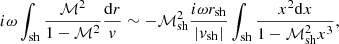
The boundary value problem is solved numerically using a shooting method from the shock to the inner boundary, iterating over the value of the complex eigenfrequency ω. The mathematical singularity at rns is overcome numerically by using logℳ as an integration variable, as in Foglizzo et al. (2007). The inner boundary is then defined as the point where the Mach number has reached a sufficiently small value (ℳ ∼ 10−9).
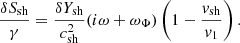
Foglizzo et al. (2007) noted similar properties of the SASI harmonics as functions of rsh/r∇ with (α, β) = (3/2, 5/2) and (6, 1) in their analysis. We extend this analysis for the fundamental mode and note in Fig. 2 that the normalised growth rate and oscillation frequency are asymptotically independent of (α, β) for rsh/r∇ ≫ 1, that is, when the cooling layer is thin compared to the shock radius. This surprising property is checked by varying (α, β) continuously from (3/2, 5/2) to (6, 1) and from (3/2, 5/2) to (5, 6) in Fig. 3. It is remarkable that the normalised oscillation frequency appears to be independent of the cooling process down to a very low ratio rsh/r∇: the following analytic formula ωrfit provides an approximation for ωr within 3% for 1.8 < rsh/r∇ < 10:
 (29)
(29)
 (30)
(30)
 (31)
(31)
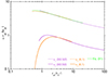 |
Fig. 2. Growth rate (solid lines) and oscillation frequency (dashed lines) of the fundamental SASI mode, normalised by |vsh|/rsh, calculated with ε = 0 for the cooling parameters (3/2, 5/2) (purple) and (6, 1) (orange), and displayed as functions of rsh/r∇. The analytic fitting formula (31) for ωr is displayed with a green dashed line. |
The adiabatic advection time  corresponds to a velocity profile increasing linearly with radius as expected asymptotically in spherical geometry for γ = 4/3 (Eq. (19) in Walk et al. 2023).
The important role of r∇ rather than rns was also noted by Scheck et al. (2008), where the strength of SASI in numerical simulations seemed correlated with the abruptness of the deceleration close to the proto-neutron star, and was confirmed in the toy model used by F09 and Guilet & Foglizzo (2012).
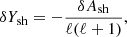
Figures 2 and 3 also show that the detailed cooling process affects the growth rate of SASI (solid lines) more than its oscillation frequency (dashed lines) when rsh < 4r∇.
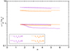 |
Fig. 3. Growth rate (solid lines) and oscillation frequency (dashed lines) of the fundamental SASI mode, normalised by |vsh|/rsh, calculated with rsh/r∇ = 2 (purple lines) and rsh/r∇ = 4 (orange lines) for a range of cooling parameters (α, β) varying continuously from (3/2, 5/2) to (6, 1) (thin lines) and from (3/2, 5/2) to (5, 6) (thick lines), as indicated in Fig. 1. |
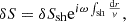
We note from Fig. 4 that the oscillation period TSASI ≡ 2π/ωr of the fundamental ℓ = 1 SASI mode can be significantly longer than the approximate advection time  for a small ratio rsh/r∇. The relationship between these two timescales is further discussed in reference to a simplified model in Sect. 5.3. The modest impact of the specificities of the parametrised cooling process on the fundamental SASI eigenfrequency encouraged us to apply our simple model to a more realistic physical model of core collapse in Sect. 2.3. We were also inspired by this finding to look for a deeper analytic understanding of the SASI mechanism using an adiabatic approximation, as detailed in Sect. 3.
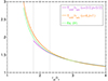 |
Fig. 4. Variation in the ratio |

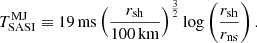
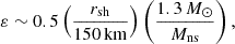
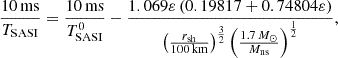
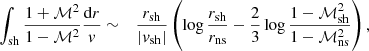
2.3. Comparison of the perturbative model with the empirical formula proposed by Müller & Janka (2014)
The adiabatic approximation of the advection time was also used in the empirical formula (33), which describes the oscillation period TSASI in the core-collapse simulation of a 25 M⊙ progenitor (Müller & Janka 2014), which is inspired by the physics of the advective-acoustic cycle. r∇ was approximated with rns and the time variation of the mass of the proto-neutron star was neglected:
 (32)
(32)
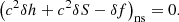
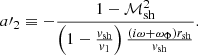
The SASI modulation of the neutrino signal was identified in their model s25 between t = 0.12 s and t = 0.45 s post-bounce. The shock radius rsh decreases from 125 km to 55 km and the ratio rsh/rns varies between 1.8 and 2.3 according to Figs. 3 and 6 of Müller & Janka (2014). The formula (32) well captures the  -dependence, which is the main source of variability of TSASI during the collapse. The overall accuracy of this formula is ∼26% for model s25 as shown in Fig. 5.
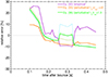 |
Fig. 5. Estimate of the relative error between the oscillation period of the neutrino signal in model s25 in Müller & Janka (2014) and in analytical estimates. The empirical formula (32) is shown with a purple line. The result of the perturbative calculation is shown for r∇ = rns without dissociation (orange line, Eq. (33)), and for r∇ = 1.3rns with dissociation prescribed by Eq. (35) (green line, Eq. (36)). The sensitivity to the estimate of r∇ is shown with dashed lines for r∇ = 1.25rns (khaki) and r∇ = 1.35rns (blue). |
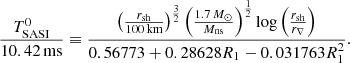
The expected variation of TSASI estimated from Eq. (31) is as follows:
 (33)
(33)
According to Fig. 5, the overall accuracy of formula (33) applied to the model s25 is improved to ∼10%, which is remarkable given the simplicity of the perturbative model, which does not involve any adjusted parameter and neglects dissociation at the shock. The mass increase Mns/M⊙ ∼ 1.7 − 2 estimated from Fig. 2 in Müller & Janka (2014) contributes to a 8% decrease in TSASI. A more physical estimate should also take into account dissociation, which can significantly increase TSASI when rsh is large, and the distinction between rns and r∇, which can significantly decrease TSASI when rsh/rns is smallest.
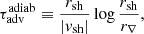
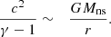
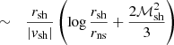
Following Fig. 6, the impact of dissociation on the oscillation frequency of SASI is tentatively approximated as
 (34)
(34)
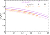 |
Fig. 6. Effect of dissociation, measured by ε, on the oscillation frequency of SASI for rsh/r∇ = 1.8 (dashed lines), 1 (solid lines), and 2.3 (dotted lines) for (α, β) = (3/2, 5/2) (purple lines) and (α, β) = (6, 1) (orange lines). The analytical formula (34) is indicated with crosses. |
We note that this analytical formula is tested only in the narrow range 1.8 < rsh/r∇ < 2.3 and is only meant to provide as an order of magnitude estimate. The dissociation parameter is approximated according to Fig. 12 in Huete et al. (2018):
 (35)
(35)
with a saturation at ε ∼ 0.5 due to partial dissociation of α-nuclei (Fernández & Thompson 2009a). Thus, Eq. (34) is rewritten as
 (36)
(36)
with
 (37)
(37)
According to Fig. 5, taking into account dissociation improves the accuracy of the empirical formula, but only for a limited range of prescribed ratio 1.25 < r∇/rns < 1.35. Improvement of the accuracy of the present perturbative model beyond the ±10% level does not appear straightforward given its many approximations regarding the microphysics, neutrino interactions, and gravity. Its main improvement compared to the empirical formula (32) is the fact that it contains physically consistent estimates of the impact of the mass, the dissociation at the shock, and the SASI phase inferred from the perturbative analysis. Each of them can potentially affect the oscillation period by several tens of percent according to Eq. (33) and Figs. 4 and 6. By neglecting these effects, the empirical formula in Eq. (32) is not expected to maintain its ∼30% accuracy for progenitors other than s25. The accuracy of Eq. (36) should be tested on other numerical simulations of core collapse, bearing in mind that our prescription for dissociation is very crude.
3. Adiabatic model
Here, the adiabatic character of the flow refers to the region between the shock and the inner boundary, while non-adiabatic processes associated to nuclear dissociation and neutrino emission are incorporated into the boundary conditions. The production of entropy perturbations by the shock displacement Δζ is taken into account. Nuclear dissociation across the shock is formally taken into account using the parameter ε (Eq. (6)), but it is set to zero in the illustrative figures of this section. The goal of the analysis presented in this section is to gain some analytical understanding of the effect of the physical parameters involved in the SASI mechanism.
3.1. Explicit expressions in the adiabatic approximation
With ℒ = 0, the differential Equations (19)–(20) describe the advection of perturbations produced by the shock. Using the boundary conditions (24), (25) with ∇S = 0:
 (38)
(38)
 (39)
(39)
Here, δSsh is defined by Eq. (24) with a simpler expression for ωΦ:
 (40)
(40)
Using Eq. (12) with δK = 0 and Eq. (38) gives the explicit expression for δw⊥ of
 (41)
(41)
The vorticity associated to the entropy perturbation is also explicitly calculated in Appendix C:
 (42)
(42)
 (43)
(43)
 (44)
(44)
Together with Eq. (12), Eqs. (43), (44) demonstrate that δK = 0 can be interpreted as a consequence of the baroclinic production of vorticity.
Equation (16) implies that the wave action δf/ω is directly related to δA:
 (45)
(45)
The transverse velocity components (δvθ, δvφ) are deduced from δA using the transverse Euler equations Eqs. (B.10), (B.11) with Eqs. (43), (44). Here, δvr is deduced from Eqs. (15) and (41):
 (46)
(46)
 (47)
(47)
 (48)
(48)
The adiabatic solution can be viewed as the asymptotic limit of the model with a cooling function when rpeak ∼ rns, corresponding to α ≪ 1 and β ≫ 1 according to Fig. 1. For the sake of simplicity, we explore the adiabatic solution with an inner boundary defined by δvr = 0, formulated by Eq. (28) with cns defined as the adiabatic sound speed at the inner boundary. This prescription could be improved to better account for non-adiabatic processes in the cooling layer. The adiabatic simulations in Blondin & Mezzacappa (2007) also used δvr = 0 at the inner boundary.
3.2. Quantitative comparison of the eigenfrequencies with and without the region of non-adiabatic cooling
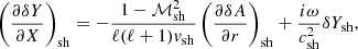
The eigenfrequencies corresponding to the adiabatic model are solved numerically and compared in Fig. 7 to the eigenfrequencies of the non-adiabatic formulation for different values of the shock radius. The overall trends suggest that the main properties of SASI can be qualitatively understood by focusing on adiabatic processes. The fundamental mode is the most unstable one for a small shock radius, and becomes dominated by higher overtones for a larger shock radius. Among the most visible differences with the non-adiabatic model, the adiabatic simplification underestimates the frequency by a factor of ≤1.3 for a large shock radius of rsh ∼ 10rns. The growth rate of the most unstable mode is overestimated by a factor of ≤1.4 for a small shock radius and is underestimated by a factor of ≤1.3 for a very large shock radius.
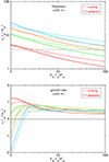 |
Fig. 7. Oscillation frequency (upper plot) and growth rate (lower plot) of the modes ℓ = 1 calculated in units of the post-shock frequency vsh/rsh, for γ = 4/3, as a function of the shock distance in the model with cooling using (α, β) = (3/2, 5/2) (dashed lines) and in the adiabatic approximation (solid lines). The fundamental mode (in red) and the first three overtones (green, orange, blue) are displayed. The grey horizontal line in the upper plot indicates the Lamb frequency at the shock. The fundamental mode becomes dominated by higher overtones as its frequency becomes too low for acoustic propagation ( |

4. Formulation of the SASI mechanism as a self-forced oscillator
4.1. Derivation of the second-order differential equation
For the sake of mathematical simplicity, we use the radial coordinate X defined as in Foglizzo (2001):
 (49)
(49)
The second-order differential Eq. (27) is simplified to
![Mathematical equation: $$ \begin{aligned} \left[\left({\partial \over \partial X}+{i\omega \over c^2}\right)^2 + {\omega ^2-\omega _{\rm Lamb}^2\over { v}^2c^2}\right]\delta A = {\partial \over \partial X} {r\delta { w}_\perp \over { v}}. \end{aligned} $$](/articles/aa/full_html/2024/12/aa52300-24/aa52300-24-eq55.gif) (50)
(50)
Using Eq. (41), the forcing term of Eq. (50) is thus proportional to the entropy perturbation δSsh produced by the shock:
![Mathematical equation: $$ \begin{aligned} \left[\left({\partial \over \partial X}+{i\omega \over c^2}\right)^2 + {\omega ^2-\omega _{\rm Lamb}^2\over { v}^2c^2}\right]{\delta A\over \ell (\ell +1)}&= -\mathcal{F}_{S}\delta S_{\rm sh} ,\end{aligned} $$](/articles/aa/full_html/2024/12/aa52300-24/aa52300-24-eq56.gif) (51)
(51)
 (52)
(52)
We show in Appendix C that the forced oscillator equation can be rewritten as follows, using boldface for vector quantities:
![Mathematical equation: $$ \begin{aligned} \left[\left({\partial \over \partial X}+{i\omega \over c^2}\right)^2 + {\omega ^2-\omega _{\rm Lamb}^2\over { v}^2c^2}\right]\delta \boldsymbol{L}&={\partial \over \partial X} {r\delta \boldsymbol{w}\over { v}} ,\end{aligned} $$](/articles/aa/full_html/2024/12/aa52300-24/aa52300-24-eq58.gif) (53)
(53)
 (54)
(54)
where δL ≡ r × δv is the perturbed specific angular momentum vector and δw ≡ ∇ × δv is the perturbed vorticity vector. We note from Eqs. (43), (44) that rv|δw|/c2 is conserved when advected. The relation between δSsh and δAsh is deduced from Eqs. (22) and (24):
 (55)
(55)
The components of transverse vorticity at the shock are related to the components of perturbed specific angular momentum according to Eqs. (43), (44) and Eqs. (47), (48):
 (56)
(56)
The boundary conditions at the shock and at the inner boundary are written in Appendix C as follows:
![Mathematical equation: $$ \begin{aligned} {\partial \delta A\over \partial X}_{\rm sh}&={i\omega \over { v}_{\rm sh}^2}\delta A_{\rm sh}\left[1-2{{{ v}_{\rm sh}}\over { v}_1} +(\gamma -1)\mathcal{M}_{\rm sh}^2 \left(1-{{{ v}_{\rm sh}}\over { v}_{1}}\right) \right]\nonumber \\&\quad -\left[1+(\gamma -1)\mathcal{M}_{\rm sh}^2\right]{\delta A_{\rm sh}\over r_{\rm sh}{ v}_{\rm sh}} \left({{ v}_1\over 2{{ v}_{\rm sh}}} -2\right), \end{aligned} $$](/articles/aa/full_html/2024/12/aa52300-24/aa52300-24-eq62.gif) (57)
(57)
 (58)
(58)
They can also be written with the variables rδvθ, rδvφ, and δwθ, δwφ, using Eqs. (43), (44) and (47), (48). Equations (51) and (53) are thus equivalent for ℓ ≥ 1. The same advective-acoustic cycle can either be considered as an entropic-acoustic cycle or as a vortical-acoustic cycle.
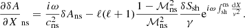
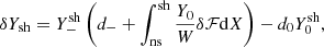
We define a new perturbative variable δY as follows:
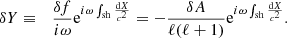 (59)
(59)
Here, Y0 is defined as the solution of the homogeneous equation associated to Eq. (51) with δS = 0 and δK = 0, and satisfying the inner boundary condition (58):
 (60)
(60)
 (61)
(61)
We refer to Y0 as the acoustic structure of the post-shock cavity modified by the radial velocity, in the absence of interaction with advected perturbations. The structure of the acoustic equation and its modification by the advection velocity v are more easily recognised when rewriting Eq. (60) with the variable r:
 (62)
(62)
Identifying the physics of SASI with a forced oscillator enables us to evaluate the efficiency of the coupling depending on two effects: (i) the amplitude of the forcing term (∝ 1/ℳ2 in Eq. (52)), and (ii) the phase match between the forcing term (advected wavelength) and the oscillator (acoustic wavelength). The forcing amplitude is strongest where ℳ is smallest, in close proximity to the proto-neutron star, but a strong phase mixing is expected there due to the decrease in the radial wavelength (∝2π|v|/ωr) of advected perturbations. A trade-off between effects (i) and (ii) favours advected perturbations with a sufficiently low frequency, coupled to the acoustic structure in a region sufficiently far from the proto-neutron star to minimize phase mixing.
This description as a forced oscillator was previously proposed in the context of radial Bondi accretion accelerated into a black hole (Foglizzo 2001, 2002) and in a planar adiabatic toy model of SASI with a localised region of feedback (F09). The present work is the first formulation where the radially extended character of the advective-acoustic coupling is taken into account in a shocked decelerated accretion flow in spherical geometry. We present a quantitative evaluation of the coupling efficiency in the following section using a classical resolution of the forced oscillator with the Wronskian method.
4.2. Integral equation defining the eigenfrequencies
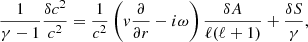
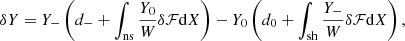
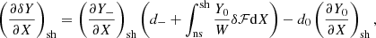
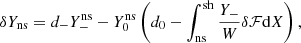
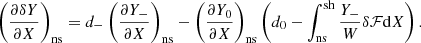
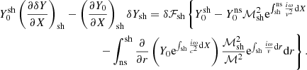
In Appendix D, we derive the integral equation defining the eigenfrequencies, which is equivalent to the full differential system and boundary conditions. It is formulated here with the variable r:
 (63)
(63)
with a′1, a′2 defined as
 (64)
(64)
 (65)
(65)
The first two terms associated with Y0 on the left-hand side of Eq. (63) are acoustic, and are marginally modified by advection. The terms on the right-hand side involve the phase oscillations of the advected perturbations. Despite the integration by part, we recognise in the integral the forcing term of Eq. (52) multiplied by the derivative of the homogeneous solution Y0. As expected in Sect. 4.1 for the classical problem of a forced harmonic oscillator, this integral characterises the efficiency of the forcing, which depends on both the amplitude profile of the forcing δℱ and the matching of its phase compared to the phase of the oscillator Y0. An analytic approximation of this integral equation is obtained in Sect. 5 in the asymptotic regime, where the acoustic radial structure is non-oscillatory. We verified numerically that the eigenfrequencies satisfying the single equation Eq. (63) are strictly the same as those obtained in Fig. 7 from the solution of the fourth-order adiabatic differential system (17), (20) with ℒ = 0, with the boundary conditions defined by Eq. (28) and Eqs. (22), (25) with ∇S = 0.
5. Analytical estimate for a large shock radius
5.1. Analytical approximations
5.1.1. Stationary flow
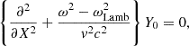
We focus on the case of a strong shock ℳ1 ≫ 1 and a large shock radius rsh ≫ rns, with the post-shock energy density described by the Bernoulli equation, Eq. (5), dominated by the enthalpy and the gravitational contributions:
 (66)
(66)
The kinetic energy density associated to the radial velocity is a minor contribution, and is even more negligible when the photodissociation across the shock is taken into account. The parameter ε impacts the post-shock Mach number and velocity according to Eqs. (A.2), (A.3):
 (67)
(67)
 (68)
(68)
![Mathematical equation: $$ \begin{aligned} {c_{\rm sh}^2r_{\rm sh}\over GM_{\rm ns}}&\sim {4\gamma (\gamma -1)(1-\varepsilon ) \over \left[2+(\gamma -1)(1-\varepsilon )\right]^2}. \end{aligned} $$](/articles/aa/full_html/2024/12/aa52300-24/aa52300-24-eq74.gif) (69)
(69)
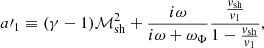
Equation (66) allows a power-law approximation of the radial velocity profile with an exponent αv deduced from Eq. (A.11). This exponent depends on both the adiabatic index and the geometry g = 2:
 (70)
(70)
 (71)
(71)
 (72)
(72)
We note that Eq. (66) is valid only for rns ≤ r ≪ rsh, and becomes inaccurate in the vicinity of the shock where the sound speed is particularly sensitive to photodissociation, as seen in Eq. (69).
5.1.2. Acoustic structure of the oscillator
Taking advantage of the low frequency of the fundamental mode for ℓ ≥ 1, we approximate in Appendix E the homogeneous solution Y0 as a linear combination of power laws independent of the frequency for ω ≪ ωLamb:
![Mathematical equation: $$ \begin{aligned} Y_0&\sim \left({r\over r_{\rm ns}}\right)^{{a}}\left[\left({r_{\rm ns}\over r}\right)^{{b}} + {{b}-{a} \over {b}+{a}} \left({r\over r_{\rm ns}}\right)^{{b}} \right], \end{aligned} $$](/articles/aa/full_html/2024/12/aa52300-24/aa52300-24-eq78.gif) (73)
(73)
![Mathematical equation: $$ \begin{aligned} {\partial Y_0\over \partial r}&\sim {{b}-{a}\over r_{\rm ns}} \left({r\over r_{\rm ns}}\right)^{{a}-1} \left[\left({r\over r_{\rm ns}}\right)^{{b}} - \left({r_{\rm ns}\over r}\right)^{{b}} \right], \end{aligned} $$](/articles/aa/full_html/2024/12/aa52300-24/aa52300-24-eq79.gif) (74)
(74)
where the exponents a, b are defined as
 (75)
(75)
![Mathematical equation: $$ \begin{aligned} {b}&\equiv \left[\left({{\alpha _{ v}}+1\over 2}\right)^2+\ell (\ell +1) \right]^{1\over 2}. \end{aligned} $$](/articles/aa/full_html/2024/12/aa52300-24/aa52300-24-eq81.gif) (76)
(76)
The exponents ±b correspond to the two components of the acoustic structure Y0, where the component decreasing inwards (+b) is associated to the evanescent profile of pressure perturbations at the shock, and the component decreasing outwards (−b) is associated to the evanescent profile of pressure perturbations at the inner boundary.
This approximate solution of Y0 satisfies the lower boundary condition only in the asymptotic limit rns ≪ rsh.
5.1.3. Forcing by advected perturbations
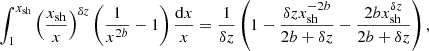
We use the following approximation of the advection time τadv(r) profile:
 (77)
(77)
![Mathematical equation: $$ \begin{aligned}&\sim {1\over \alpha _{ v}-1}{r_{\rm sh}\over |{ v}_{\rm sh}|}\left[\left({r_{\rm sh}\over r}\right)^{\alpha _{ v}-1}-1\right]\;\;\mathrm{if}\;\;\alpha _{ v}\ne 1,\end{aligned} $$](/articles/aa/full_html/2024/12/aa52300-24/aa52300-24-eq83.gif) (78)
(78)
 (79)
(79)
In particular, Eq. (79) is applicable for γ = 4/3. In this regime, the advection time τadv is asymptotically dominated by the inner region. A numerical calculation indicates that this analytical formula slightly underestimates the adiabatic advection time by less than 6% in the range 1 < rsh/rns < 100.
We examine the accuracy of our approximation of ℳ and Y0 in Fig. 8.
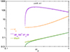 |
Fig. 8. Solution of the homogeneous equation Y0 associated with the fundamental mode ℓ = 1 (solid orange line) for rsh/rns = 5. This solution is very well approximated analytically by Eq. (73) (dashed orange line with crosses). The radial profile of the amplitude of the forcing term in Eq. (63) (purple solid line) is compared to its analytical approximation (dashed purple line with crosses) using Eqs. (72) and (74). The Mach number profile in the adiabatic model (green solid line) is compared to its analytical approximation (Eq. (72), green dashed line with crosses). The Mach profile of the flow including cooling is shown for reference (dark green line). |
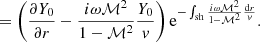
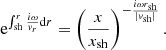
5.2. Analytical expression of the fundamental eigenfrequency
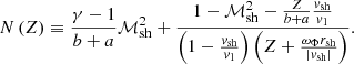
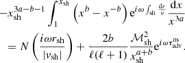
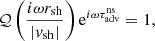
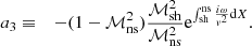
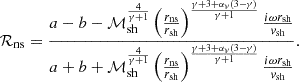
We approximate Eq. (63) using Eq. (72) and Eq. (73) with ℳ2 ≪ 1, except near the shock. We use the approximations (73) and (74) of Y0 and ∂Y0/∂r and note that (∂log Y0/∂log r)sh ∼ 1/(b + a) with a, b defined by Eqs. (75) and (76). We define N ≡ a2′+a1′/(b + a) and introduce the normalised eigenfrequency Z ≡ iωrsh/|vsh|:
 (80)
(80)
Using the variable x ≡ r/rns, for ℓ ≥ 1 the eigenfrequency equation, Eq. (63), is approximated by
 (81)
(81)
The approximation of the eigenfrequency with γ = 4/3 allows an explicit calculation of the integral involved in Eq. (81). The following equation defining the eigenfrequencies for ℓ ≥ 1 is expressed using the complex amplification factor 𝒬(ω) per advective-acoustic cycle:
![Mathematical equation: $$ \begin{aligned} \mathcal{Q}(Z)&\equiv {2{b} \left({r_{\rm sh}\over r_{\rm ns}}\right)^{2-{b}} \left\{ 1+\left[(Z+2)^2-{b}^2 \right]{\mathcal{M}_{\rm sh}^2\over \ell (\ell +1) x_{\rm sh}^3} \right\} \over \left[1 -\left(Z+2-{b}\right) N \right]\left(Z+2+{b}\right) -{Z+2-{b}\over x_{\rm sh}^{2{b}}} } , \end{aligned} $$](/articles/aa/full_html/2024/12/aa52300-24/aa52300-24-eq87.gif) (82)
(82)
 (83)
(83)
where b2 = 1 + ℓ(ℓ + 1) and the advection time  from the shock to the inner boundary is approximated by Eq. (79). The numerical solution of this equation is compared to the exact solution of Eq. (63) in Fig. 9.
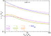 |
Fig. 9. Eigenfrequency of the adiabatic solution (green lines) based on the integral formulation (63) compared to its integrated approximation (83) (orange lines), which is based on the approximate description of the flow profile v,ℳ and acoustic structure Y0. The estimate of the oscillation frequency |

The good agreement obtained with the analytic expression (83) demonstrates that the approximation of the flow profile v, ℳ and the approximation of the homogeneous solution Y0 are sufficient to capture the essence of the instability in the adiabatic model and identify the leading contributions in the integral expression (63). The frequency is overestimated by up to 20% and the growth rate is overestimated by up to 26%. The region of radial propagation of acoustic waves was neglected for the sake of simplicity in the analytical approximation (73) of Y0, without significant consequences regarding the approximation of the fundamental frequency ωr, because the radial extension of this region is modest compared to the region affecting the phase of advected perturbations.
The larger inaccuracy of ∼76% of the simple formula  , also shown in Fig. 9, is mainly due to the neglect of the frequency dependence of the phase of 𝒬, denoted φ𝒬. The complex Eq. (83) is equivalent to the following set of two real equations:
 (84)
(84)
 (85)
(85)
5.3. Oscillation period of the advective-acoustic cycle in the adiabatic approximation
Comparing ωr and  in Fig. 9, it is particularly striking that the oscillation period TSASI ≡ 2π/ωr is significantly longer than the adiabatic advection time
  . This contrasts with the simulations in Scheck et al. (2008) where
  , in line with the analytic toy model of F09. Not only does TSASI differ from
  by more than 76%, but TSASI is actually 76% longer than the longest advection timescale
  , excluding the possibility that the oscillation period could coincide with any advection time. As explained in Scheck et al. (2008), the relation between TSASI and
  does depend on the phase φ𝒬 of the complex efficiency 𝒬.
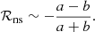
The adiabatic approximation teaches us that, even in a simple adiabatic model, the phase shift φ𝒬 should not be neglected a priori. This was also true in the calculation of Sect. 2.3 with non-adiabatic cooling. The value of |𝒬| and φ𝒬 can be deduced from ω and  from Eqs. (84), (85):
 (86)
(86)
 (87)
(87)
This characterisation of the fundamental eigenfrequency is calculated in Fig. 10 in the adiabatic approximation and compared to the analytical estimate deduced from Eqs. (82), (83); for reference, it is also displayed in the flow with cooling, using the same adiabatic advection time, which should not be confused with the actual advection time taking into account the cooling layer. In the adiabatic flow, the winding angle of the spiral pattern of advected perturbations from the shock to the neutron star is  . We note in Fig. 10 that φ𝒬 < π, implying that the radial structure of advected perturbations of entropy or vorticity contains at least a change of sign, as seen in Fig. 2 of Blondin & Shaw (2007), Fig. 1 of Fernández (2010), and Fig. 10 of Buellet et al. (2023).
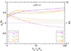 |
Fig. 10. Amplitude |𝒬| (solid lines) and normalised phase φ𝒬/2π (dashed lines) of the complex amplification factor associated through Eqs. (86), (87) to the fundamental eigenfrequency ω calculated with cooling (purple lines with crosses) and in the adiabatic approximation (green lines), using the same adiabatic estimate of the advection time |

5.4. Comparison to the analytic model in Foglizzo (2009)
The adiabatic formulation incorporates major improvements compared to the adiabatic toy model used by F09, Sato et al. (2009), Guilet & Foglizzo (2012): the plane parallel model allows for explicit analytical solutions and a deeper understanding of the instability mechanism, but some simplifications are difficult to justify: (i) the assumption of a uniform flow between the shock and the region of deceleration implies that the vertical size of the acoustic and advected cavities are identical, thus overestimating the impact of radial acoustic propagation on the phase of the solution; (ii) the maximum strength 𝒬 ∼ 2 of the advective-acoustic cycle is arbitrarily set by the specific value (0.75) chosen for the ratio csh2/cout2, which limits the relative effect of the purely acoustic cycle on the most unstable modes; (iii) the optimum value of the vertical wavenumber compared to the horizontal one is set by the specific value chosen for L/H = 4 in F09 and Sato et al. (2009) and L/H = 6 in Guilet & Foglizzo (2012; iv) the width of the coupling region described by H∇/H is also a free parameter of the model.
The present adiabatic model offers a new framework overcoming these shortcomings, and is still simple enough to allow for analytical results:
– The spherical geometry is taken into account (rather than a plane parallel approximation in F09).
– The adiabatic heating and deceleration are produced in a self-consistent manner by the radial convergence in 3D and by the proto-neutron star gravity (rather than being localised at the lower boundary by some external potential with adjustable depth csh2/cout2 and width H∇/H in F09).
– The gravity produced by the neutron star at the shock is not neglected, allowing both displacement and velocity effects for the production of entropy at the shock (rather than ignoring displacement effects with ωΦ = 0 in F09).
The adiabatic model sheds light on some objections by Blondin & Mezzacappa (2006) regarding the advective-acoustic mechanism in a non-rotating flow:
(i) The fact that the advection time may be longer than the oscillation period does not contradict the advective-acoustic mechanism.
(ii) The fact that the pressure field shows no evidence for a radially localised coupling radius is explained by the radially extended character of the coupling process, as seen in the integral in Eq. (63). The feedback should refer to the radially extended pressure structure rather than the radial propagation of an acoustic wave.
6. Conclusions and perspectives
-
The oscillation period of the fundamental SASI mode can be estimated from the shock radius rsh, the radius of maximum deceleration r∇, and the central mass Mns.
-
A possible improvement to the analytic formula used by Müller & Janka (2014) is proposed, based on the perturbative analysis without any adjustment of a specific numerical simulation.
-
An adiabatic model of the shock dynamics incorporating non-adiabatic processes in the boundary conditions is able to capture the general properties of SASI eigenmodes.
-
In the adiabatic approximation, the SASI mechanism can be described as a self-forced oscillator. The forcing by advected perturbations is distributed from the shock surface to the cooling layer rather than inside the cooling layer.
-
An analytical description of the properties of the fundamental mode of SASI in the adiabatic approximation is obtained in the asymptotic limit of a large ratio rsh/r∇.
Improving the accuracy of the estimation of the SASI oscillation period from a perturbative analysis requires (i) a more accurate prescription for partial dissociation at the shock and in the flow, as described in Appendix A of Fernández & Thompson (2009a), and (ii) a better characterisation of the parametrised cooling function, leading to a realistic value of the ratio r∇/rns.
The adiabatic framework proposed here opens a new path for analytical investigation of the physical effect of stellar rotation in the equatorial plane (Paper II), and provides a means to address the intriguing results of Walk et al. (2023), which they obtained by comparing SASI properties in cylindrical and spherical geometries.
We note that the adiabatic approximation indeed accounts for the growth rate and oscillation period within ∼30%, leaving room for additional non-adiabatic effects. By decreasing the velocity and Mach number near the proto-neutron star, the amplitude of the forcing term is increased, as is the phase mixing near the proto-neutron star. In addition to affecting the trade-off between these two effects, non-adiabatic effects modify the amplitude of δS and δK during their advection, add a source of feedback in the cooling layer, and modify the acoustic equation. A quantitative assessment of some of these effects can be obtained within the formalism of the self-forced oscillator by incorporating them into the lower boundary condition.
Acknowledgments
The anonymous referee is thanked for constructive suggestions. It is a pleasure to acknowledge stimulating discussions with Jérôme Guilet, Matteo Bugli, Thomas Janka, Bernhard Müller, Kei Kotake, Tomoya Takiwaki, Ernazar Abdikamalov, Laurie Walk, Irene Tamborra, Anne-Cécile Buellet, Sonia El Hedri, Florent Robinet and the LEAK collaboration funded by the LabEx UnivEarthS. This work has been financially supported by the PNHE.
References
- Blondin, J. M., & Mezzacappa, A. 2006, ApJ, 642, 401 [NASA ADS] [CrossRef] [Google Scholar]
- Blondin, J. M., & Mezzacappa, A. 2007, Nature, 445, 58 [CrossRef] [PubMed] [Google Scholar]
- Blondin, J. M., & Shaw, S. 2007, ApJ, 656, 366 [NASA ADS] [CrossRef] [Google Scholar]
- Blondin, J. M., Mezzacappa, A., & DeMarino, C. 2003, ApJ, 584, 971 [NASA ADS] [CrossRef] [Google Scholar]
- Blondin, J. M., Gipson, E., Harris, S., & Mezzacappa, A. 2017, ApJ, 835, 170 [NASA ADS] [CrossRef] [Google Scholar]
- Buellet, A. C., Foglizzo, T., Guilet, J., & Abdikamalov, E. 2023, A&A, 674, A205 [NASA ADS] [CrossRef] [EDP Sciences] [Google Scholar]
- Burrows, A., & Vartanyan, D. 2021, Nature, 589, 29 [CrossRef] [PubMed] [Google Scholar]
- Drago, M., Andresen, H., Di Palma, I., Tamborra, I., & Torres-Forné, A. 2023, Phys. Rev. D, 108, 103036 [NASA ADS] [CrossRef] [Google Scholar]
- Dunham, S. J., Endeve, E., Mezzacappa, A., et al. 2024, ApJ, 964, 38 [NASA ADS] [CrossRef] [Google Scholar]
- Fernández, R. 2010, ApJ, 725, 1563 [CrossRef] [Google Scholar]
- Fernández, R., & Thompson, C. 2009a, ApJ, 703, 1464 [CrossRef] [Google Scholar]
- Fernández, R., & Thompson, C. 2009b, ApJ, 697, 1827 [CrossRef] [Google Scholar]
- Fernández, R., Müller, B., Foglizzo, T., & Janka, H.-T. 2014, MNRAS, 440, 2763 [CrossRef] [Google Scholar]
- Foglizzo, T. 2001, A&A, 368, 311 [NASA ADS] [CrossRef] [EDP Sciences] [Google Scholar]
- Foglizzo, T. 2002, A&A, 392, 353 [NASA ADS] [CrossRef] [EDP Sciences] [Google Scholar]
- Foglizzo, T. 2009, ApJ, 694, 820 [NASA ADS] [CrossRef] [Google Scholar]
- Foglizzo, T., Galletti, P., & Ruffert, M. 2005, A&A, 435, 397 [NASA ADS] [CrossRef] [EDP Sciences] [Google Scholar]
- Foglizzo, T., Scheck, L., & Janka, H. T. 2006, ApJ, 652, 1436 [NASA ADS] [CrossRef] [Google Scholar]
- Foglizzo, T., Galletti, P., Scheck, L., & Janka, H. T. 2007, ApJ, 654, 1006 [NASA ADS] [CrossRef] [Google Scholar]
- Foglizzo, T., Masset, F., Guilet, J., & Durand, G. 2012, Phys. Rev. Lett., 108, 051103 [NASA ADS] [CrossRef] [Google Scholar]
- Foglizzo, T., Kazeroni, R., Guilet, J., et al. 2015, PASA, 32, e009 [NASA ADS] [CrossRef] [Google Scholar]
- Guilet, J., & Foglizzo, T. 2012, MNRAS, 421, 546 [Google Scholar]
- Huete, C., Abdikamalov, E., & Radice, D. 2018, MNRAS, 475, 3305 [CrossRef] [Google Scholar]
- Janka, H.-T. 2017, ApJ, 837, 84 [Google Scholar]
- Janka, H.-T., Melson, T., & Summa, A. 2016, Ann. Rev. Nucl. Part. Sci., 66, 341 [Google Scholar]
- Kitaura, F. S., Janka, H. T., & Hillebrandt, W. 2006, A&A, 450, 345 [NASA ADS] [CrossRef] [EDP Sciences] [Google Scholar]
- Kotake, K., & Kuroda, T. 2017, in Handbook of Supernovae, eds. A. W. Alsabti, & P. Murdin, 1671 [CrossRef] [Google Scholar]
- Müller, B. 2019a, MNRAS, 487, 5304 [CrossRef] [Google Scholar]
- Müller, B. 2019b, Ann. Rev. Nucl. Part. Sci., 69, 253 [CrossRef] [Google Scholar]
- Müller, B. 2020, Liv. Rev. Comput. Astrophys., 6, 3 [Google Scholar]
- Müller, B., & Janka, H.-T. 2014, ApJ, 788, 82 [CrossRef] [Google Scholar]
- Müller, B., Tauris, T. M., Heger, A., et al. 2019, MNRAS, 484, 3307 [Google Scholar]
- Powell, J., & Müller, B. 2022, Phys. Rev. D, 105, 063018 [NASA ADS] [CrossRef] [Google Scholar]
- Sato, J., Foglizzo, T., & Fromang, S. 2009, ApJ, 694, 833 [NASA ADS] [CrossRef] [Google Scholar]
- Scheck, L., Janka, H. T., Foglizzo, T., & Kifonidis, K. 2008, A&A, 477, 931 [NASA ADS] [CrossRef] [EDP Sciences] [Google Scholar]
- Stockinger, G., Janka, H. T., Kresse, D., et al. 2020, MNRAS, 496, 2039 [Google Scholar]
- Tamborra, I., & Murase, K. 2019, Supernovae. Ser.: Space Sci. Ser. ISSI, 68, 87 [NASA ADS] [Google Scholar]
- Walk, L., Foglizzo, T., & Tamborra, I. 2023, Phys. Rev. D, 107, 063014 [NASA ADS] [CrossRef] [Google Scholar]
Appendix A: Stationary accretion
The loss of energy through nuclear dissociation is measured by the parameter ε defined by Eq. (6). It decreases the value of the post-shock Mach number ℳsh below the reference adiabatic value ℳad, and affects the Rankine-Hugoniot conditions according to Eqs. (A4-A6) of Foglizzo et al. (2006):
 (A.1)
(A.1)
 (A.2)
(A.2)
 (A.3)
(A.3)
 (A.4)
(A.4)
The nuclear binding energy of the iron nuclei is 8.8MeV per nucleon, or 1.77 × 1052erg/M⊙. If nuclear dissociation was complete across the shock this would translates into a dissociation parameter scaling linearly with rsh:
 (A.5)
(A.5)
We note that our definition of ε in Eq. (6) follows Huete et al. (2018), which differs from Eq. (4) in Fernández & Thompson (2009b) by a factor 2. A fraction of the dissociation of iron nuclei is radially distributed between the shock and the neutron star surface, as calculated in Fernández & Thompson (2009a). Taking into account incomplete dissociation, the value of ϵ formulated in Eq. (35) is a rough estimate deduced from Eq. (51) and Fig. 12 in Huete et al. (2018) for rsh < 175km. It is smaller than Eq. (A.5) by a factor ∼1.4 and saturates at ϵ ∼ 0.5 in exploding models.
The value of ℳsh is expressed as a function of ℳ1 and ε(rsh) using Eq. (A.2):
![Mathematical equation: $$ \begin{aligned} {\mathcal{M}_{\rm sh}^2\over \mathcal{M}_{\rm ad}^2}&= {1\over 2} + { 1-{2\varepsilon \over 1+{2\over \gamma -1}{1\over \mathcal{M}_1^2}}-{\mathcal{M}_{\rm ad}^2\over 2\mathcal{M}_1^2} \over 1+\left[\left(1-{\mathcal{M}_{\rm ad}^2\over \mathcal{M}_1^2}\right)^2+{4\varepsilon {\mathcal{M}_{\rm ad}^2\over \mathcal{M}_1^2}\over 1+{2\over \gamma -1}{1\over \mathcal{M}_1^2}} \right]^{1\over 2} } ,\end{aligned} $$](/articles/aa/full_html/2024/12/aa52300-24/aa52300-24-eq110.gif) (A.6)
(A.6)
 (A.7)
(A.7)
The jump condition (A.3) is thus a function of ε(rsh) using Eq. (A.6), with the simple following expression for a strong shock:
 (A.8)
(A.8)
 (A.9)
(A.9)
The definition of the cooling function (1), the dimensionless entropy (2) and the mass conservation (3) are used to eliminate the variables  from the stationary equations, Eqs. (4) and (5):
 (A.10)
 (A.11)
Appendix B: Differential system and boundary conditions of the perturbed accretion
We rewrite the differential system satisfied by δf, δh (Eqs. (E2-E3) in Foglizzo et al. (2006)), using the radial coordinate X defined as in Foglizzo (2001):
 (B.1)
(B.1)
Thus
 (B.2)
(B.2)
 (B.3)
(B.3)
The set of equations Eqs. (A1)-(A4) in Foglizzo et al. (2007) are repeated here for completeness:
 (B.4)
(B.4)
 (B.5)
(B.5)
 (B.6)
(B.6)
 (B.7)
(B.7)
![Mathematical equation: $$ \begin{aligned} \delta \left( {\mathcal{L}\over \rho { v}} \right)&= \nabla S {c^2\over \gamma } \left[(\beta - 1) {\delta \rho \over \rho } + \alpha {\delta c^2\over c^2} - {\delta { v}_r\over { v}} \right]\ , \end{aligned} $$](/articles/aa/full_html/2024/12/aa52300-24/aa52300-24-eq124.gif) (B.8)
(B.8)
![Mathematical equation: $$ \begin{aligned} \delta \left( {\mathcal{L}\over p { v}} \right)&= \nabla S \left[(\beta - 1) {\delta \rho \over \rho } + (\alpha -1) {\delta c^2\over c^2} - {\delta { v}_r\over { v}} \right]. \end{aligned} $$](/articles/aa/full_html/2024/12/aa52300-24/aa52300-24-eq125.gif) (B.9)
(B.9)
The perturbed mass conservation and transverse components of the perturbed Euler equation are:
 (B.10)
 (B.11)
We eliminate δvθ and δvφ in the system of Eqs. (12), (14), (B.10) and (B.11) and obtain Eq. (16).
The derivative of δA is calculated using Eqs. (16), (20) and (B.2), leading to the differential system (17-20) satisfied by δA, δh, δS, δK. The second derivative of δA is calculated using Eqs. (12), (20) and (B.3), resulting in Eq. (27).
Using Eq. (16), Eqs. (B.4-B.7) are rewritten as follows:
 (B.12)
 (B.13)
 (B.14)
 (B.15)
Using Eq. (B.12) with Eq. (12), we can express δvr with δA and δw⊥ and obtain Eq. (15). We note that this relation is equivalent to the radial component of the vector calculus relation ∇2v = ∇(∇ ⋅ v)−∇×(∇ × v).
The baroclinic production of vorticity by the advection of entropy perturbations can be calculated in the same way as Eqs. (E17-E19) in Foglizzo et al. (2005), using the conservation of the tangential component of the velocity across the shock:
 (B.16)
 (B.17)
The vorticity produced at the shock is defined by Eqs. (B.16-B.17), the transverse components (B.10-B.11) of the Euler equation at the shock, together with the angular derivative of Eqs. (22):
 (B.18)
![Mathematical equation: $$ \begin{aligned} \delta { w}_{\theta \mathrm{sh}}&= - {c_{\rm sh}^2\over \gamma }{im\over r_{\rm sh}{ v}_{\rm sh}\sin \theta } \left(\delta S_{\rm sh}+\left[\nabla S\right]^\mathrm{sh}_{1} \Delta \zeta \right), \end{aligned} $$](/articles/aa/full_html/2024/12/aa52300-24/aa52300-24-eq135.gif) (B.19)
(B.19)
![Mathematical equation: $$ \begin{aligned} \delta { w}_{\varphi \mathrm{sh}}&= {c_{\rm sh}^2\over \gamma } {1\over r_{\rm sh}{ v}_{\rm sh}} {\partial \over \partial \theta }\left(\delta S_{\rm sh}+\left[\nabla S\right]^\mathrm{sh}_{1} \Delta \zeta \right). \end{aligned} $$](/articles/aa/full_html/2024/12/aa52300-24/aa52300-24-eq136.gif) (B.20)
(B.20)
Appendix C: Adiabatic model
Following Eqs. (B5)-(B7) in Foglizzo (2001), the differential equation describing the specific vorticity in a spherical adiabatic flow can be integrated as
 (C.1)
(C.1)
![Mathematical equation: $$ \begin{aligned} \delta { w}_\theta&= {1\over rv}\left[(rv\delta { w}_\theta )_{\rm sh} -{c^2-c_{\rm sh}^2\over \sin \theta }im{\delta S_{\rm sh}\over \gamma }\right]\mathrm{e}^{i\omega \int _{\rm sh}{\mathrm{d}r\over { v}}} ,\end{aligned} $$](/articles/aa/full_html/2024/12/aa52300-24/aa52300-24-eq138.gif) (C.2)
(C.2)
![Mathematical equation: $$ \begin{aligned} \delta { w}_\varphi&= {1\over rv}\left[(rv\delta { w}_\varphi )_{\rm sh} +{c^2-c_{\rm sh}^2\over \sin \theta }{\partial \over \partial \theta }{\delta S_{\rm sh}\over \gamma }\right]\mathrm{e}^{i\omega \int _{\rm sh}{\mathrm{d}r\over { v}}}. \end{aligned} $$](/articles/aa/full_html/2024/12/aa52300-24/aa52300-24-eq139.gif) (C.3)
(C.3)
Using Eqs. (B.18-B.20) with ∇S = 0, together with Eqs. (C.1-C.3) gives the expression (42-44) of the vorticity perturbation throughout the flow.
With δY defined by Eq. (59), the expressions of δAsh, δhsh are deduced from Eqs. (22-24):
 (C.4)
(C.4)
 (C.5)
(C.5)
 (C.6)
(C.6)
We rewrite Eq. (17) using the definitions of X and δY with δK = 0:
 (C.7)
(C.7)
![Mathematical equation: $$ \begin{aligned} \left({\partial \delta A\over \partial r}\right)_{\rm sh} ={\ell (\ell +1){ v}_{\rm sh}\over 1-\mathcal{M}_{\rm sh}^2}\left[\delta Y_{\rm sh}{i\omega \over { v}_{\rm sh}^2}\left({{{ v}_{\rm sh}}\over { v}_1}+\mathcal{M}_{\rm sh}^2\right) \right.\nonumber \\ \left. -{\delta S_{\rm sh}\over \gamma }\left({1\over \mathcal{M}_{\rm sh}^2}+\gamma -1\right)\right],\end{aligned} $$](/articles/aa/full_html/2024/12/aa52300-24/aa52300-24-eq144.gif) (C.8)
(C.8)
 (C.9)
(C.9)
which results in Eq. (57).
At the inner boundary in the adiabatic approximation, we use the condition δvr = 0:
 (C.10)
The entropy is simply advected from the shock (38) and we express δh with δY and ∂δY/∂X using Eq. (17):
 (C.11)
 (C.12)
The inner boundary condition (C.10) is thus reduced to Eq. (58).
Multiplying Eq. (51) by m/(ω sin θ) and using Eqs. (43) and (48):
![Mathematical equation: $$ \begin{aligned} \left[\left({\partial \over \partial X}+{i\omega \over c^2}\right)^2 + {\omega ^2-\omega _{\rm Lamb}^2\over { v}^2c^2}\right]r\delta { v}_\varphi =-{\partial \over \partial X} {r\delta { w}_\theta \over { v}}. \end{aligned} $$](/articles/aa/full_html/2024/12/aa52300-24/aa52300-24-eq149.gif) (C.13)
(C.13)
Equivalently, using Eq. (44) and (47) and the derivative of Eq. (51) with respect to θ leads to:
![Mathematical equation: $$ \begin{aligned} \left[\left({\partial \over \partial X}+{i\omega \over c^2}\right)^2 + {\omega ^2-\omega _{\rm Lamb}^2\over { v}^2c^2}\right]r\delta { v}_\theta ={\partial \over \partial X} {r\delta { w}_\varphi \over { v}}, \end{aligned} $$](/articles/aa/full_html/2024/12/aa52300-24/aa52300-24-eq150.gif) (C.14)
(C.14)
which is equivalent to Eq. (C.13) given the spherical symmetry of the stationary flow.
Appendix D: Equation defining the eigenfrequencies in the adiabatic model
The differential equation satisfied by δY is deduced from Eqs. (51) and (59):
 (D.1)
(D.1)
 (D.2)
(D.2)
We define Y0 as the solution of the homogeneous equation satisfying the inner boundary condition of pure acoustic waves (i.e. without entropy and vorticity perturbations), and Y− another homogeneous solution such that their Wronskien is W:
 (D.3)
(D.3)
 (D.4)
(D.4)
 (D.5)
(D.5)
where  is the forcing term on the right hand side of Eq. (51) for the variable δY defined by. Using Eq. (D.5) at the upper boundary:
 (D.6)
(D.6)
 (D.7)
(D.7)
Using Eq. (D.5) at the lower boundary:
 (D.8)
(D.8)
 (D.9)
(D.9)
Using Eq. (D.3), the lower boundary condition (58) translates into
![Mathematical equation: $$ \begin{aligned} d_-\left[\left({\partial Y_-\over \partial X}\right)_{\rm ns} - {i\omega \over c_{\rm ns}^2} Y_-^\mathrm{ns}\right]= \delta \mathcal{F}_{\rm sh}(1-\mathcal{M}^2_{\rm ns}){\mathcal{M}_{\rm sh}^2\over \mathcal{M}^2_{\rm ns}}\mathrm{e}^{\int _{\rm sh}^\mathrm{ns} {i\omega \over { v}^2}\mathrm{d}X}. \end{aligned} $$](/articles/aa/full_html/2024/12/aa52300-24/aa52300-24-eq161.gif) (D.10)
(D.10)
We note using Eq. (D.4) and (D.3) that
 (D.11)
Thus
 (D.12)
Eliminating d0 between Eqs. (D.6) and (D.7) and using Eq. (D.4):
![Mathematical equation: $$ \begin{aligned} Y_0^\mathrm{sh}\left({\partial \delta Y\over \partial X}\right)_{\rm sh}-\left({\partial Y_0\over \partial X}\right)_{\rm sh} \delta Y_{\rm sh} =\nonumber \\ \left[Y_0^\mathrm{sh}\left({\partial Y_-\over \partial X}\right)_{\rm sh}-\left({\partial Y_0\over \partial X}\right)_{\rm sh}Y_-^\mathrm{sh}\right]\left(d_-+\int _{\rm ns}^\mathrm{sh}{ Y_0\over W} \delta \mathcal{F}\mathrm{d}X\right),\end{aligned} $$](/articles/aa/full_html/2024/12/aa52300-24/aa52300-24-eq164.gif) (D.13)
(D.13)
 (D.14)
The eigenfrequencies are thus defined by
 (D.15)
Replacing the forcing term by its expression (D.2),
 (D.16)
Using Eqs. (24) and (57) this equation takes the form
 (D.17)
with a1, a2, a3 defined by:
 (D.18)
 (D.19)
 (D.20)
 (D.21)
 (D.22)
After one integration by parts:
 (D.23)
The equation defining the eigenfrequencies becomes Eq. (63) with a′1 ≡ a1 − 1 and a′2 ≡ a2 defined by Eqs. (64-65).
Appendix E: Approximation of the adiabatic stationary flow and the homogeneous perturbative solution
The dissociation measured by the parameter ε affects the relation between |vsh| and the local free fall velocity, as deduced from Eq. (68) for a strong shock:
 (E.1)
(E.1)
 (E.2)
(E.2)
Equation (E.2) is transformed into Eq. (69) using Eqs. (E.1) and (67). We use a power law approximation of the enthalpy profile deduced from the Bernoulli equation for r ≪ rsh and ℳ2 ≪ 1:
![Mathematical equation: $$ \begin{aligned} c^2\left[1+(\gamma -1){\mathcal{M}^2\over 2}\right]=(\gamma -1){GM_{\rm ns}\over r}\nonumber \\ +c_{\rm sh}^2\left[1+(\gamma -1){\mathcal{M}_{\rm sh}^2\over 2}\right]-(\gamma -1){GM_{\rm ns}\over r_{\rm sh}},\end{aligned} $$](/articles/aa/full_html/2024/12/aa52300-24/aa52300-24-eq177.gif) (E.3)
(E.3)
 (E.4)
(E.4)
The mass conservation and the adiabatic hypothesis in Eq. (A.11) imply the power law approximations (71) and (72) for the velocity and Mach number profiles.
For γ = 4/3 we approximate
 (E.5)
(E.5)
 (E.6)
(E.6)
 (E.7)
(E.7)
 (E.8)
(E.8)
The oscillatory phase associated to δf in Eq. (63) is made of a product of (iω) with two explicit contributions and a third contribution from the definition of δY in Eq. (59). The sum of these three contributions is:
 (E.9)
(E.9)
With αv = 1 and  ,
,
 (E.10)
The integral can be estimated as follows:
 (E.11)
 (E.12)
With a strong adiabatic shock  , the correction to the advection timescale
  is thus of order 12% for rsh/rns = 2 and 5% for rsh/rns = 5. This correction is smaller if dissociation diminishes the value of
  .
.
The contribution of the integral inside the radial derivative in Eq. (63) is limited to a contribution of order  :
:
 (E.13)
![Mathematical equation: $$ \begin{aligned}&\sim&{\omega r_{\rm sh}\over |{ v}_{\rm sh}|} {\mathcal{M}_{\rm sh}^2\over \alpha _{ v}+2}\left[1-\left({r\over r_{\rm sh}}\right)^{\alpha _{ v}+2}\right]. \end{aligned} $$](/articles/aa/full_html/2024/12/aa52300-24/aa52300-24-eq193.gif) (E.14)
(E.14)
With ωr ∼ 2π|vsh|/rsh for a small shock radius this phase shift is not negligible since it reaches 0.74 ∼ π/4 at the inner boundary and it is linear in ω.
We integrate Eq. (49) using Eq. (71) and neglecting ℳ2 ≪ 1:
 (E.15)
 (E.16)
The two solutions Y0± of the homogeneous equation (60) are approximated as power laws with exponents α±.
 (E.17)
Injecting Y0±(r) into Eq. (60),
![Mathematical equation: $$ \begin{aligned} {\alpha _\pm }\left({\alpha _\pm }- \alpha _{ v}-1\right)\left({r\over r_{\rm sh}}\right)^{- 2{\alpha _{ v}}-2} = \nonumber \\ -\left[{\omega ^2 r_{\rm sh}^2\over c^2}-\ell (\ell +1) {r_{\rm sh}^2\over r^2}\right]\left({{ v}_{\rm sh}\over { v}}\right)^2. \end{aligned} $$](/articles/aa/full_html/2024/12/aa52300-24/aa52300-24-eq197.gif) (E.18)
(E.18)
For ℓ ≥ 1, the restoring force in Eq. (60) is independent of the frequency in the region where ω ≪ ωLamb. Thus, using Eq. (E.4) for ℓ ≥ 1,
 (E.19)
 (E.20)
In this region the approximate solution is α± ≡ a ± b with a, b defined by Eqs. (75) and (76). The homogeneous solution Y0 for ℓ ≥ 1 is a linear combination of power laws Y0± satisfying the lower boundary condition (61):
 (E.21)
 (E.22)
With ℳns ≪ 1 and using Eq. (72),
 (E.23)
 (E.24)
From Eq. (E.24) we conclude that the coefficient ℛns is asymptotically independent of ω when rns ≪ rsh.
 (E.25)
The acoustic function is independent of the frequency in the asymptotic limit rns ≪ rsh for low frequency perturbations ℓ ≥ 1 driven by advection such that ωrsh/|vsh|≤1, as described by Eqs. (73) and (74).
Using the index 0 to denote the acoustic perturbation associated to the homogeneous solution, we note from Eqs. (46) with δS = 0 and Eq. (59) that the relation between ∂Y0/∂r and δvr0 is
 (E.26)
 (E.27)
The fact that Eq. (74) imposes ∂Y0/∂r = 0 is approximately compatible with δvr0 ∼ 0 to the extent that ℳns ≪ 1.
Appendix F: Approximation of the eigenfrequency equation for γ = 4/3
The advection time for αv = 1 is approximated using Eq. (79):
 (F.1)
(F.1)
Defining δz ≡ iωrsh/|vsh|+2 − b and noting that a = 1, the leading terms in Eq. (81) for ℓ ≥ 1 are :
 (F.2)
(F.2)
The integral on the right hand side can be calculated explicitly. If δz ≠ 0,
 (F.3)
(F.3)
Using Eq. (F.3) in Eq. (F.2) we obtain the following equation defining δz:
![Mathematical equation: $$ \begin{aligned} \left[1- \delta z N({b}-2+\delta z) \right]\left(1+{\delta z\over 2{b}}\right) -{\delta z\over 2{b} x_{\rm sh}^{2{b}}} = \nonumber \\ x_{\rm sh}^{\delta z } \left[1 + \delta z {2{b}\mathcal{M}_{\rm sh}^2 \over \ell (\ell +1)x_{\rm sh}^{3}} \left(1+{\delta z\over 2{b}}\right) \right]. \end{aligned} $$](/articles/aa/full_html/2024/12/aa52300-24/aa52300-24-eq210.gif) (F.4)
(F.4)
Reintroducing the normalised eigenfrequency Z = iωrsh/|vsh|,
![Mathematical equation: $$ \begin{aligned} {x_{\rm sh}^{{b}-2}\over 2{b}} \left\{ \left[1- \left(Z+2-{b}\right) N\left(Z\right) \right]\left(Z+2+{b}\right) -{Z+2-{b}\over x_{\rm sh}^{2{b}}} \right\} = \nonumber \\ x_{\rm sh}^{Z} \left\{ 1 + \left[\left(Z+2\right)^2-{b}^2 \right]{\mathcal{M}_{\rm sh}^2 \over \ell (\ell +1)x_{\rm sh}^{3}} \right\} . \end{aligned} $$](/articles/aa/full_html/2024/12/aa52300-24/aa52300-24-eq211.gif) (F.5)
(F.5)
The approximate advection time  from the shock to the inner boundary, defined by Eq. (79), is introduced to obtain Eqs. (82-83).
All Figures
|
Fig. 1. Ratios rpeak/rns (thick solid lines) and r∇/rns (thin dotted lines) depending on the coefficients (α, β) that define the cooling function in Eq. (1). The contour lines are calculated for γ = 4/3 in spherical geometry, with rsh/rns = 10, without dissociation (ε = 0). The values of rpeak/rns and r∇/rns are indicated with the same colour code. The cooling parameters (α, β) = (3/2, 5/2), (6, 1) and (5, 6) used in Fig. 3 are indicated with crosses for reference and are connected by grey lines. The black dotted line marks the threshold β = α above which the advection time from rpeak to rns is finite and r∇ = rns. |
| In the text | |
|
Fig. 2. Growth rate (solid lines) and oscillation frequency (dashed lines) of the fundamental SASI mode, normalised by |vsh|/rsh, calculated with ε = 0 for the cooling parameters (3/2, 5/2) (purple) and (6, 1) (orange), and displayed as functions of rsh/r∇. The analytic fitting formula (31) for ωr is displayed with a green dashed line. |
| In the text | |
|
Fig. 3. Growth rate (solid lines) and oscillation frequency (dashed lines) of the fundamental SASI mode, normalised by |vsh|/rsh, calculated with rsh/r∇ = 2 (purple lines) and rsh/r∇ = 4 (orange lines) for a range of cooling parameters (α, β) varying continuously from (3/2, 5/2) to (6, 1) (thin lines) and from (3/2, 5/2) to (5, 6) (thick lines), as indicated in Fig. 1. |
| In the text | |
|
Fig. 4. Variation in the ratio |
| In the text | |
|
Fig. 5. Estimate of the relative error between the oscillation period of the neutrino signal in model s25 in Müller & Janka (2014) and in analytical estimates. The empirical formula (32) is shown with a purple line. The result of the perturbative calculation is shown for r∇ = rns without dissociation (orange line, Eq. (33)), and for r∇ = 1.3rns with dissociation prescribed by Eq. (35) (green line, Eq. (36)). The sensitivity to the estimate of r∇ is shown with dashed lines for r∇ = 1.25rns (khaki) and r∇ = 1.35rns (blue). |
| In the text | |
|
Fig. 6. Effect of dissociation, measured by ε, on the oscillation frequency of SASI for rsh/r∇ = 1.8 (dashed lines), 1 (solid lines), and 2.3 (dotted lines) for (α, β) = (3/2, 5/2) (purple lines) and (α, β) = (6, 1) (orange lines). The analytical formula (34) is indicated with crosses. |
| In the text | |
|
Fig. 7. Oscillation frequency (upper plot) and growth rate (lower plot) of the modes ℓ = 1 calculated in units of the post-shock frequency vsh/rsh, for γ = 4/3, as a function of the shock distance in the model with cooling using (α, β) = (3/2, 5/2) (dashed lines) and in the adiabatic approximation (solid lines). The fundamental mode (in red) and the first three overtones (green, orange, blue) are displayed. The grey horizontal line in the upper plot indicates the Lamb frequency at the shock. The fundamental mode becomes dominated by higher overtones as its frequency becomes too low for acoustic propagation ( |
| In the text | |
|
Fig. 8. Solution of the homogeneous equation Y0 associated with the fundamental mode ℓ = 1 (solid orange line) for rsh/rns = 5. This solution is very well approximated analytically by Eq. (73) (dashed orange line with crosses). The radial profile of the amplitude of the forcing term in Eq. (63) (purple solid line) is compared to its analytical approximation (dashed purple line with crosses) using Eqs. (72) and (74). The Mach number profile in the adiabatic model (green solid line) is compared to its analytical approximation (Eq. (72), green dashed line with crosses). The Mach profile of the flow including cooling is shown for reference (dark green line). |
| In the text | |
|
Fig. 9. Eigenfrequency of the adiabatic solution (green lines) based on the integral formulation (63) compared to its integrated approximation (83) (orange lines), which is based on the approximate description of the flow profile v,ℳ and acoustic structure Y0. The estimate of the oscillation frequency |
| In the text | |
|
Fig. 10. Amplitude |𝒬| (solid lines) and normalised phase φ𝒬/2π (dashed lines) of the complex amplification factor associated through Eqs. (86), (87) to the fundamental eigenfrequency ω calculated with cooling (purple lines with crosses) and in the adiabatic approximation (green lines), using the same adiabatic estimate of the advection time |
| In the text | |
Current usage metrics show cumulative count of Article Views (full-text article views including HTML views, PDF and ePub downloads, according to the available data) and Abstracts Views on Vision4Press platform.
Data correspond to usage on the plateform after 2015. The current usage metrics is available 48-96 hours after online publication and is updated daily on week days.
Initial download of the metrics may take a while.