© The Authors 2024

1. Introduction

New in situ observations by the Parker Solar Probe (PSP) in the young solar wind confirm an extended presence of the core-beam tandem in the observed proton velocity distributions (Klein et al. 2021; Verniero et al. 2022). The motivation for theoretical and numerical modeling of these populations thus becomes even stronger, especially for understanding the origin of proton beams (PBs), but also for determining their implications for the solar wind plasma dynamics (Klein et al. 2021; Verniero et al. 2022; Ofman et al. 2022; Krasnoselskikh et al. 2023). Existing scenarios (that do not necessarily agree among each other) claim that PBs can be injected by magnetic reconnection events at the coronal base, but can also result from the trapping and acceleration of protons by resonant waves, such as cyclotron or even kinetic Alfvén waves (Marsch 2006; Araneda & Marsch 2008; Pierrard & Voitenko 2010; Krasnoselskikh et al. 2023). An immediate consequence of PBs is self-generated wave instabilities, which are expected to convert the bulk kinetic energy to smaller scales because the resulting wave fluctuations can subsequently dissipate and heat the solar wind plasma (Marsch 2006; Bale et al. 2019; Bowen et al. 2020). Favorable evidence emerges from PSP data regarding the source of the PBs and their regularization by self-induced instabilities (Bowen et al. 2020; Verniero et al. 2022; Phan et al. 2022). Moreover, observations of PBs simultaneous with ion-scale wave fluctuations (Klein et al. 2021; Verniero et al. 2020) complement data from Helios, Wind, and STEREO, for example, and facilitate concluding the long debate of whether right-handed (RH) magnetosonic (MS) modes dominate left-handed (LH) ion-cyclotron (IC) waves at 1 AU, while the latter can be dominant closer to the Sun due to the temperature anisotropy in the proton core (Marsch et al. 1982; Daughton & Gary 1998; Gary et al. 2016; Woodham et al. 2019). When the core becomes stable, which is mostly due to collisional effects, the beam becomes the dominant emitter of wave power (see Yoon et al. (2024) and references therein). Depending on their properties, the PBs can destabilize either RH-MS modes or the LH-IC instability. The generation of RH wave fluctuations seems to be the more complex process and is still an open question (Verniero et al. 2020).

This Letter shows that the PB firehose-like instabilities of RH transverse waves can determine a broad relaxation of the beams so that the beams resemble the hammerhead distributions reported by PSP (Verniero et al. 2022). Moreover, these RH transverse waves are predominantly associated with core beam structures that were observed by PSP (Klein et al. 2021). Section 2 explains the moment-based quasi-linear (QL) formalism of the transverse instabilities induced by the drifting bi-Maxwellian proton population. Although the assumption of a fixed shape for the velocity distribution function, specifically, a superposition of two drifting bi-Maxwellian distributions, limits the QL framework, it serves as an effective toy model for preliminary investigations. The simplicity and computational efficiency of a simplified moment-based QL approach make it very handy compared to more advanced numerical simulations, in particular, which typically require extensive time and computational resources. Our motivation for using the QL theory lies in its ability to provide rapid insights into the underlying physical processes despite its limitations. This toy model effectively characterizes kinetic instabilities and their effects on the relaxation of anisotropic distributions (Shaaban et al. 2019b,a; Yoon et al. 2024), and the results were often confirmed by advanced simulations, proving the validity of the theoretical approach (Pavan et al. 2011; Seough et al. 2015; Lee et al. 2018; Sarfraz et al. 2021; López et al. 2023)

The parameterization used here for the proton populations is realistic and consistent with observations. Section 3 discusses several relevant results from our parametric analysis and provides a semiquantitative comparison with the observations. Growing waves partially convert the free (kinetic) energy of the PB into the heating of this component mainly in the perpendicular direction. The properties of RH waves and the resulting temperature anisotropy, A_b = T_b⊥/T_b∥ > 1 (∥, ⊥ are gyrotropic directions concerning the background magnetic field), also conform to the observations (Verniero et al. 2022). The last section summarizes the results and draws the main conclusions of this Letter.

2. QL approach to the PB instability

In the proton (subscript p) velocity distribution,

$$\begin{array}{c}\hfill f_p(v_{\Vert },v_{\perp })=\frac{n_c}{n_p}{f}_c(v_{\Vert },v_{\perp })+\frac{n_b}{n_p}{f}_b(v_{\Vert },v_{\perp }),\end{array}$$(1)

the core (subscript c) and beam (subscript b) components are both assumed to be well described by drifting bi-Maxwellian distributions,

$$\begin{array}{cc}\hfill f_j(v_{\Vert },v_{\perp })=& \frac{{\pi }^{-3/2}}{{\alpha }_{\perp j}^2{\alpha }_{\Vert j}}exp[-\frac{v_{\perp }^2}{{\alpha }_{\perp a}^2}-\frac{{(v_{\Vert }-v_j)}^2}{{\alpha }_{\Vert a}^2}].\hfill \end{array}$$(2)

n_c and n_b are the core and beam number density, respectively, and n_p = n_b + n_c is the total number density of the protons. α_{j ∥ ,⊥}(t) = [2k_BT_{j ⊥ ,∥}(t)/m_p]^1/2 are components of the thermal velocities, while v_j are drift velocities, which preserve a zero net current n_cv_c = n_bv_b. According to our QL approach, these velocities vary in time (t) as a measure of energy exchange. Electrons (subscript e) ensure a neutral plasma (n_e = n_p). They are nondrifting (v_e = 0) and are initially isotropic and Maxwellian distributed.

For this plasma configuration, the (instantaneous) dispersion relation for the RH transverse modes that propagate parallel to the magnetic field reads (Shaaban et al. 2020)

$$\begin{array}{cc}\hfill {\stackrel{\sim }{k}}^2=& {\delta }_c[{\mathrm{\Psi }}_c+{\mathrm{\Gamma }}_{c+}^{+}{Z}_c\left({\xi }_c^{+}\right)]+{\delta }_b[{\mathrm{\Psi }}_b+{\mathrm{\Gamma }}_{b-}^{+}{Z}_b\left({\xi }_b^{+}\right)]\hfill \\ \hfill & +\mu [{\mathrm{\Psi }}_e+{\mathrm{\Gamma }}_e^{-}{Z}_e\left({\xi }_e^{-}\right)],\hfill \end{array}$$(3)

where $\stackrel{\sim }{k}=ck/{\omega }_{\mathit{pp}}$ is the normalized wavenumber, c is the speed of light, ω_pp = (4πn_pe²/m_p)^1/2 is the proton plasma frequency, $\stackrel{\sim }{\omega }=\omega /{\mathrm{\Omega }}_p$ is the normalized wave frequency, Ω_j =  eB₀/m_jc is the nonrelativistic gyro-frequency of the plasma species j (with elementary charge e), β_j∥ = 8πn_jk_BT_j∥/B₀² are the parallel plasma beta parameters, Ψ_j = A_j − 1, A_j = T_j⊥/T_j∥ ≡ β_j⊥/β_j∥ is the temperature anisotropy, μ = m_p/m_e is the proton-electron mass ratio, $U_j=V_j/\sqrt{{\delta }_c}$, V_b = v_b/v_Ac, ${\mathit{v}}_{\mathit{Ac}}=B_0/\sqrt{4\pi n_c{m}_p}$ is the proton core Alfvén speed, $Z_j\left({\xi }_j^{\pm }\right)$ is the plasma dispersion function (Fried & Conte 1961) of arguments

$$\begin{array}{c}\hfill {\xi }_{j\mp }^{+}=\frac{\stackrel{\sim }{\omega }+1\mp \stackrel{\sim }{k}{U}_j}{\stackrel{\sim }{k}\sqrt{{\beta }_{j\Vert }/{\delta }_j}},{\xi }_e^{-}=\frac{\stackrel{\sim }{\omega }-\mu }{\stackrel{\sim }{k}\sqrt{\mu {\beta }_{e\Vert }}},\end{array}$$

and

$$\begin{array}{cc}\hfill {\mathrm{\Gamma }}_{j\mp }^{+}=& \frac{A_j(\stackrel{\sim }{\omega }+1\mp \stackrel{\sim }{k}{U}_j)-1}{\stackrel{\sim }{k}\sqrt{{\beta }_{j\Vert }/{\delta }_j}},{\mathrm{\Gamma }}_e^{-}=\frac{A_e(\stackrel{\sim }{\omega }-\mu )+\mu }{\stackrel{\sim }{k}\sqrt{\mu {\beta }_{e\Vert }}}.\hfill \end{array}$$

The QL evolution of the macroscopic parameters (moments of f_j), such as the plasma betas β_⊥, ∥j and drifting velocities V_j, is governed by the following equations:

$$\begin{array}{cc}\hfill \frac{\mathrm{d}{\beta }_{j\perp }}{\mathrm{d}\tau }=& -{\delta }_j{\displaystyle \int }\frac{\mathrm{d}\stackrel{\sim }{k}}{{\stackrel{\sim }{k}}^2}W(\stackrel{\sim }{k})[{\mathrm{\Lambda }}_j\stackrel{\sim }{\gamma }+G_{j\perp }^{\pm }{\eta }_{j\mp }^{\pm }],\hfill \end{array}$$(4a)

$$\begin{array}{cc}\hfill \frac{\mathrm{d}{\beta }_{j\Vert }}{\mathrm{d}\tau }=& 2{\delta }_j{\displaystyle \int }\frac{\mathrm{d}\stackrel{\sim }{k}}{{\stackrel{\sim }{k}}^2}W(\stackrel{\sim }{k})[A_j\stackrel{\sim }{\gamma }+G_{j\Vert }{\eta }_j^{\pm }],\hfill \end{array}$$(4b)

$$\begin{array}{cc}\hfill \frac{\mathrm{d}{V}_b}{\mathrm{d}\tau }=& \frac{\sqrt{{\delta }_c}}{2}{\displaystyle \int }\frac{\mathrm{d}\stackrel{\sim }{k}}{\stackrel{\sim }{k}}W(\stackrel{\sim }{k})\mathrm{Im}{\eta }_{b-}^{+}/\left(\stackrel{\sim }{k}\sqrt{{\beta }_{b\Vert }/{\delta }_b}\right),\hfill \end{array}$$(4c)

$$\begin{array}{cc}\hfill \frac{\mathrm{d}{V}_c}{\mathrm{d}\tau }=& \frac{-\sqrt{{\delta }_c}}{2}{\displaystyle \int }\frac{\mathrm{d}\stackrel{\sim }{k}}{\stackrel{\sim }{k}}W(\stackrel{\sim }{k})\mathrm{Im}{\eta }_{c+}^{+}/\left(\stackrel{\sim }{k}\sqrt{{\beta }_{c\Vert }/{\delta }_c}\right),\hfill \end{array}$$(4d)

in terms of τ = Ω_pt, the instantaneous growth rate $\stackrel{\sim }{\gamma }(t)=\gamma /{\mathrm{\Omega }}_p$ derived from the linear dispersion relation (3), the normalized wave (spectral) energy density $W(\stackrel{\sim }{k})=\delta B^2(\stackrel{\sim }{k})/B_0^2$, and

$$\begin{array}{cc}\hfill {\delta }_j& =n_j/n_e,{\mathrm{\Lambda }}_j=(2A_j-1),{\mathrm{\Lambda }}_e=\mu (2A_e-1)\hfill \end{array}$$(5a)

$$\begin{array}{cc}\hfill {\eta }_{j\mp }^{+}& =[A_j(\stackrel{\sim }{\omega }\mp \stackrel{\sim }{k}{U}_j)+(A_j-1)]Z_j\left({\xi }_{j\mp }^{+}\right),\hfill \end{array}$$(5b)

$$\begin{array}{cc}\hfill {\eta }_e^{-}& =\mu [A_e\stackrel{\sim }{\omega }-(A_e-1)\mu ]Z_e\left({\xi }_e^{-}\right),\hfill \end{array}$$(5c)

$$\begin{array}{cc}\hfill G_{j\perp }^{+}& =\mathrm{Im}\frac{2i\stackrel{\sim }{\gamma }+1}{\stackrel{\sim }{k}\sqrt{{\beta }_{j\Vert }/{\delta }_j}},G_{e\perp }^{-}=\mathrm{Im}\frac{2i\stackrel{\sim }{\gamma }-\mu }{\stackrel{\sim }{k}\sqrt{\mu {\beta }_{e\Vert }}},\hfill \end{array}$$(5d)

$$\begin{array}{cc}\hfill G_{j\Vert \mp }^{+}& =\mathrm{Im}\frac{\stackrel{\sim }{\omega }+1\mp \stackrel{\sim }{k}{U}_j}{\stackrel{\sim }{k}\sqrt{{\beta }_{j\Vert }/{\delta }_j}},G_{e\Vert }^{-}=\mathrm{Im}\frac{\stackrel{\sim }{\omega }-\mu }{\stackrel{\sim }{k}\sqrt{\mu {\beta }_{e\Vert }}}.\hfill \end{array}$$(5e)

The wave equation completes the QL equations,

$$\begin{array}{c}\hfill \frac{\partial W_t(\stackrel{\sim }{k})}{\partial \tau }=2\stackrel{\sim }{\gamma }(\tau )W_t(\stackrel{\sim }{k}).\end{array}$$(6)

To obtain these equations, we used the standard QL formalism, which is similar to those by Seough & Yoon (2012), Moya et al. (2012), Sarfraz et al. (2016), Yoon (2017).

3. Results supporting the formation of the hammerhead PB

We discuss the numerical results from the linear and QL analysis for 15 runs with different initial parameters. We list the parameters below.

Runs 1, 2, 3: |V_b(0)| = 3.0, 2.5, 2.0,

Runs 4, 5, 6: |V_b(0)| = 3.0,  n_b/n_p = 0.06, 0.03, 0.01,

Runs 7, 8, 9: |V_b(0)| = 2.0,  β_c∥(0) = 1.0, 0.41, 0.1,

Runs 10, 11, 12: |V_b(0)| = 4.5,  A_b(0) = 2.0, 1.0, 0.62.

Runs 13, 14, 15 in Figure 3: |V_b(0)| = 4.5.0, 4.0, 3.5.

The other initial values we used for the plasma parameters were $W(\stackrel{\sim }{k})={10}^{-6}$, A_j(0) = 1, n_b/n_p = 0.02, β_c∥(0) = 0.41, and T_b∥/T_c∥ = 2.465, unless otherwise specified. These are estimates from the PSP observations, for example, in Klein et al. (2021), Verniero et al. (2022).

3.1. Linear analysis

The dispersion relation (3) was solved exactly numerically to derive the unstable solutions of the RH-PB mode, whose growth rates ($\stackrel{\sim }{\gamma }$) are displayed in Figure 1 (the panels in the top row) as a function of the wave number ($\stackrel{\sim }{k}$). The growth rates are systematically enhanced, especially when the beam drift velocity |v_b/v_Ac| is increased (left panel) and for the beam density n_b/n_p (second panel). The stimulation also consists of expanding the range of unstable mode wavenumbers. The increase in the beam temperature in the perpendicular direction has a similar but less significant effect (fourth panel). When the beam velocity is higher, the growth rate may combine the peaks of the RH and LH modes (Shaaban et al. 2020). The variation in the growth rates is less monotonic, it increases and then decreases with the plasma beta (third panel). This is specific to beam instabilities of electromagnetic or transverse modes (Shaaban et al. 2018, 2020). In this case, a PB firehose-like instability develops between two threshold conditions, between the regime of electrostatic instabilities for a low-beta parameter (or thermal spread) and the regime of ion-cyclotron instabilities for a high-beta parameter (or thermal spread). The wave frequency of the unstable mode (not shown here) displayed minor variations when the plasma parameters were changed. We also note that the unstable solutions derived from the RH dispersion relation (3), that is, with ${\xi }_{b,c}^{+}$, have positive wave frequencies (ω_r/Ω_p > 0) for $\stackrel{\sim }{k}>0$. This confirms their RH polarization.

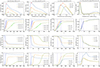Fig. 1. Numerical solutions from linear theory and QL approach: Growth rates ($\stackrel{\sim }{\gamma }$) of the RH-PB instability (top) and the corresponding time evolutions for the wave energy density (second row), beam velocity (third row), and the beam temperature anisotropy (bottom) for different initial conditions: vb/vAc = 3.0, 2.5, 2.0 (left column), nb/np = 0.06, 0.03, 0.01 (second column), βc∥ = 1.0, 0.41, 0.1 (third column), and Ab = 2.0, 1.0, 0.62 (right column). The red dots and dashed and dotted lines are explained in the text.

3.2. QL analysis

In addition to the linear theory, we resolved the set of QL equations (4)–(6) for the initial parameters (i.e., at τ₀ = 0) of each run indicated above. The results in Figure 1 first show the time evolution of the RH-PB wave energy density W_t(τ)≡δB²/B₀² (second row). The next rows lower describe the back reaction of the growing waves on the macroscopic plasma parameters, such as the beam velocity |v_b(τ)/v_Ac| (third row) and the induced beam temperature anisotropy A_b(τ). Each corresponds to the initial growth rates displayed in the first top panels, with the same color style. In Figure 1 we mark the maximum growth rates (red dots), which correspond to the fastest-growing modes, and use their values, that is, γ_m, to estimate the QL growth of the energy density of these modes, shown by the dashed lines (second row) with the slope given by 2γ_m. The dashed lines reproduce the increase in QL of the wave energy density with a high accuracy in many cases. This demonstrates that the linear theory and the QL formalism agree sufficiently well. In addition, two relevant times are marked (for clarity, only blue runs, including run 4 invoked in Figure 2). Namely, τ₁ for the beginning of the beam velocity relaxation (corresponding to the increase in the beam anisotropy), and τ₂ marks the end of the QL increase in the wave energy density as the temporal (maximum) limit up to which we can compute the resonance paths.

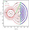Fig. 2. Contours of proton VD for run 4 at τ = 0 (dashed gray) and at τ = 31 (solid red), when the forward-half of VD is shaped by the kinetic shells (blue) that were found relevant for the hammerhead populations reported by PSP (Verniero et al. 2022). The diffusion contours v⊥(v∥) were computed by linking the proton coordinates (v∥, v⊥) (green squares) with the resonant wave frame (vϕ, r/vA = 1.3, 0.0) (black dot) and ${\stackrel{\sim }{k}}_r=0.60$. The slope of these lines, such as the green line, is v⊥/[v∥ − vϕ], with v∥ and v⊥ calculated using Eqs. (14) and (15) in Isenberg & Lee (1996).

We first discuss runs 1–3, which show the variations with the beam velocity, and the results of which are displayed in the left column of Figure 1 for |v_b(0)/v_Ac| = 3.0 (blue), 2.5 (orange), and 2.0 (green). An increase in the initial |v_b(0)/v_Ac| can determine not only a faster initiation (blue line), but also higher levels of the RH-PB fluctuations (second panel). This confirms the stimulation of the instability as predicted by linear theory (top panel). The excitation of RH-PB fluctuations regulates the free energy of the PB populations, reducing the beam velocity or relative drift (third panel), and also through the preferential cooling and heating mechanisms of the beam population. The relaxation of the drift velocity is accompanied by perpendicular heating of the beam and a relatively high anisotropy T_b⊥ > T_b∥ (bottom panel) that is reached at (or slightly before) the instability saturation. These effects are more prominent and faster for more energetic beams with a higher initial velocity. For example, the beam that initially has |v_b(0)/v_Ac| = 3.0 loses ∼25% after relaxation, whereas beams with |v_b(0)/v_Ac| = 2.5 and 2.0 lose ∼14% and ∼9%, respectively. Moreover, the initially isotropic protons of the beam component, with A_b(0) = 1.0, experience a stronger perpendicular heating (blue line) when their initial |v_b(0)/v_Ac| is higher, resulting in a significant induced temperature anisotropy at later stages, that is, A_b(τ_max)≃2.9 for |v_b(0)/v_Ac| = 3.0.

The second (left) column in Figure 1 displays the results from runs 4, 5, and 6, which correspond to different initial number densities of the beam, n_b/n_p = 0.06 (blue), 0.03 (orange), and 0.01 (green). The panels show the temporal profile of the wave energy density of RH-PB fluctuations (second panel), their back reactions on the beam drift velocity |v_b(τ)/v_Ac| (third panel), and the beam temperature anisotropy A_b(τ) (bottom). Denser beams are more efficient in shortening the instability onset time and in stimulating the fluctuation growth to higher levels after saturation. This also confirms the predictions from linear theory. As a result, the relaxation of the beam velocity |v_b(τ)/v_Ac| becomes faster and deeper, simultaneously with a strong induced (perpendicular) temperature anisotropy A_b > 1 (even after the saturation). However, the (maximum) induced anisotropy A_b > 1 is lower for denser beams, and this agrees with the observational data collected by PSP that were reported by Verniero et al. (2022) (see panel (a) of Figure 2 therein).

In Figure 2 we plot the contours of the proton velocity distribution as an example, initially at τ₀ = 0 (dashed gray) and τ₂ = 31 (solid red). This corresponds to the results from run 4 in Figure 1 (second left column, blue curves). The beam population relaxes to lower drift velocities, but also gains temperature anisotropy in the perpendicular direction. The blue contours represent the resonance paths or kinetic shells, which we computed as in Verniero et al. (2022). They were used to explain the primary QL diffusion of protons resulting from the interaction with RH-PB waves from high energies in the parallel direction toward less populated regions at higher pitch angles. Although we used the cold-plasma (yet dispersive) approximation (see also Isenberg & Lee (1996)), kinetic shells shape the forward profiles of the red contours quite well¹. It appears that our moment-based QL model of the RH-PB instability, although it is a simplified approach (even by assuming idealized Maxwellian distributions), can explain the hammerhead features reported by PSP quite well, and it performs much better than first attempts in numerical simulations (Pezzini et al. 2024).

The third column from the left in Figure 1 displays the QL results for runs 7, 8, and 9 for different initial values of the core parallel beta β_c∥(0) = 1.0 (blue), 0.41 (orange), and 0.1 (green), respectively. The temporal profiles of the wave energy density (second row) and the PB parameters do not change much. However, their dependence on the initial values of β_c∥(0) is less uniform, as we also found for the linear growth rates. For instance, the faster onset and maximum level of the enhanced fluctuation are associated with β_c∥(0) = 0.41, in agreement with the peaking growth rate (top panel) from linear theory. However, for the same run 8, the drift velocity relaxation and the induced temperature anisotropy (orange lines) reach intermediate values compared to the other two cases. Moreover, the deeper relaxation of the beam drift velocity is associated with the lowest induced anisotropy (blue lines) in run 7 with β_c∥(0) = 1.0, and vice versa in run 9 (green lines) with β_c∥(0) = 0.1.

The right (last) column in Figure 1 displays the QL results for runs 10, 11, and 12 for different initial beam anisotropies, A_b = 2.0 (blue), 1.0 (orange), and 0.62 (green), respectively. The differences obtained for the saturated levels of the unstable fluctuations (second panel) and the relaxation of the beam velocity (third panel) are insignificant. However, the induced beam temperature anisotropies for each run are notable. In particular, A_b > 6 was reached at the saturation of run 10 (which started already with an A_b(0) = 2), and A_b ≃ 4 was reached at the saturation of run 12.

3.3. Constraints on the observed hammerhead populations

The dynamic paths of the beam temperature anisotropy A_b(τ) > 1 that are induced by the RH-PB instability as a function of relative beam velocity v_b − c(τ)/v_Ac are displayed for all 15 runs in Figure 3 in the left and right panels. The initial states in the (A_b, v_b − c/v_Ac) space are shown with black squares, and the magnetic wave energy (δB²/B₀²) level is color-coded (rainbow scheme). The final states after saturation are described in the figure. These temporal profiles show the relaxation of the beam drift velocity toward lower values concomitant with the heating of the (initially isotropic) beam protons in the perpendicular direction, which end with a high anisotropy A_b(τ) > 1 at later times after saturation. These effects are a direct consequence of the enhanced RH-PB electromagnetic fluctuations and are consistent with the observations collected by PSP, see the right panel and Figure 2 in Verniero et al. (2022). In the right panel, we directly compare the dynamic paths with the observations, by superimposing the QL paths on the PSP events relevant for the hammerhead populations reported by Verniero et al. (2022) in panel (b) of their Figure 2. The occurrence rate of the hammerhead distributions (normalized to the total number of events and color-coded on the right-side bar) was computed during the 7 h ion-scale wave storm. This can be interpreted as a measure of the perpendicular velocity-space diffusion strength. According to the adopted instrumental convention, a negative drift velocity was chosen for the orientation of the magnetic field.

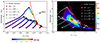Fig. 3. Comparison between QL theory and PSP observations. Left: QL dynamical paths of the temperature anisotropy (Ab) vs. beam-core drift velocity (vb − c/vAc). The black squares are the initial states, and the magnetic wave energy level is color-coded. The final states after saturation gather on the red curve (see text): red (large) dots for runs 1–3 and 13–15, circles for runs 4–6, black triangles for runs 7–9, and green triangles for runs 10–12. Right: Same as the left panel (black symbols are now shown as white symbols), but superimposed on PSP observations. The (normalized) number of events with hammerhead populations are color-coded (adapted from Figure 2, panel (b), in Verniero et al. (2022) ©AAS).

Thus, all the dynamic paths follow the same trend: They pass through the specific states of the hammerhead distributions, even the distributions with the highest occurrence rate. After the instability saturation, the final states align along the following marginal stability condition (red curve in Figure 3):

$$\begin{array}{c}\hfill A_b=1+a{(-v_{b-c}/v_{\mathit{Ac}})}^b,\end{array}$$(7)

with a = 0.0019 and b = 8.04. These states also correspond to the highest levels of the wave energy density (color-coded in the left panel). This threshold precisely bounds the events characterized by the hammerhead distributions (right panel in Figure 3), which is an exceptional result.

The regimes that are stable against the RH-PB instability are located on the right side of the stability threshold (red line), as indicated by the black arrow. These states occur when the drift velocities are annihilated by the temperature anisotropies in the perpendicular direction, regardless of whether both are small or tend to be large. On the other (left) side of the stability threshold, the RH-PB instability is active, and there is a wave-particle energy exchange. This is also suggested by the increase in the wave energy density. It is also worth mentioning that the final states of 10 out of the 15 runs settle down and accumulate in relatively narrow parametric intervals A_b = [1.8, 2.9], and v_b − c/v_Ac = [ − 2.3, −2.2], as indicated within the dashed oval. These appear to be the most likely quasi-stable states against the RH-PB instability predicted by our QL theory for the plasma conditions reported by the PSP observations. The mean values of the beam drift velocity and the perpendicular temperature anisotropy corresponding to the events with hammerhead proton distributions are v_b − c/v_Ac ≈ 2.5 and A_b ≈ 2.5 (Verniero et al. 2022), which also agree well with our QL results.

4. Conclusions

The new in situ data from the young solar wind obtained by the PSP are expected to provide unprecedented details of the plasma dynamics at temporal resolutions superior to those of other missions. In this Letter, we have investigated the formation conditions of the so-called hammerhead population, which is associated with core-beam distributions of protons from PSP measurements (Verniero et al. 2022). We proposed a relatively simple QL approach for the RH-PB instability that provides sufficient evidence of its involvement in the generation of such a hammerhead distribution through direct action on the PB relaxation. Depending on the initial conditions chosen according to the PSP observations, the energy density of the resulting waves can reach a few percent (up to around 10 %) of the energy density of the (uniform) magnetic field. The growing RH-PB waves convert the PBs bulk energy, but also scatter the protons and reduce the beam drift, and prompt diffusion in velocity space. On the timescale of the QL interaction, one can highlight the pitch-angle diffusion toward less populated regions and the agreement between the kinetic shells and the forward contours of the distributions in Figure 2. These kinetic shells are typical of the hammerhead populations observed by PSP (Verniero et al. 2022) and thus provide a plausible explanation for the formation of these populations from the interaction of PBs with the self-generated waves. Next, on longer timescales, preferential heating of the PB also takes place, leading to a significant temperature anisotropy in the perpendicular direction, A_b = T_b⊥/T_b∥ > 1 (Figure 1). For all runs, the core protons and the electrons also gain energies in the perpendicular direction. Still, the maximum values we obtained do not exceed 12% of the initial values, for instance, A_c, e(τ_max) increases from 1.0 to 1.12. Our results strongly suggest that the third hammerhead population is not necessarily distinct, but is intimately related to the beam. The model proposed here naturally results from the diffusion of beam protons induced by the instability in velocity space in the direction perpendicular to the magnetic field (Figure 2).

The importance of our results is further highlighted by the exceptional agreement with the observational data (Figure 3, right panel). First of all, RH transverse waves are predominantly associated with core-beam structures observed by PSP, even for neighboring time intervals (Klein et al. 2021). Second, but even more striking, the QL dynamic paths obtained for different initial parameters pass through the PSP events that are relevant to hammerhead populations. Moreover, the marginal stability, Equation (7), predicted by our QL approach shapes the margins of these unstable events very well. Thus, we can conclude that these hammerhead distributions are rather transient states that are still subject to relaxation mechanisms, in which kinetic (self-generated) instabilities such as the one discussed here are very likely involved. While our moment-based QL framework is limited by its assumption that the bi-Maxwellian shape of VDF is fixed, it is an effective toy model for preliminary investigations. The simplicity and facilities of our QL approach make it an effective tool for preliminary studies. This sets the stage for more detailed investigations using numerical simulation. Our results should stimulate the refinement of existing numerical simulations and settings to capture the formation of hammerhead distributions and confirm QL predictions.

Acknowledgments

The authors acknowledge support from the Ruhr-University Bochum, the Katholieke Universiteit Leuven, and Qatar University. These results were also obtained in the framework of the projects C14/19/089 (C1 project Internal Funds KU Leuven), G002523N (FWO-Vlaanderen), SIDC Data Exploitation (ESA Prodex), Belspo project B2/191/P1/SWiM. P.H.Y. acknowledges the support by NASA Awards 80NSSC19K0827, 80NSSC23K0662, the Department of Energy grant DE-SC0022963 through the NSF/DOE Partnership in Basic Plasma Science and Engineering, NSF Grant 2203321, to the University of Maryland. The authors also thank the reviewer, Dr. Mihailo Martinovic, for constructive criticism and suggestions.

References

All Figures

Fig. 1. Numerical solutions from linear theory and QL approach: Growth rates ($\stackrel{\sim }{\gamma }$) of the RH-PB instability (top) and the corresponding time evolutions for the wave energy density (second row), beam velocity (third row), and the beam temperature anisotropy (bottom) for different initial conditions: vb/vAc = 3.0, 2.5, 2.0 (left column), nb/np = 0.06, 0.03, 0.01 (second column), βc∥ = 1.0, 0.41, 0.1 (third column), and Ab = 2.0, 1.0, 0.62 (right column). The red dots and dashed and dotted lines are explained in the text.

In the text

Fig. 2. Contours of proton VD for run 4 at τ = 0 (dashed gray) and at τ = 31 (solid red), when the forward-half of VD is shaped by the kinetic shells (blue) that were found relevant for the hammerhead populations reported by PSP (Verniero et al. 2022). The diffusion contours v⊥(v∥) were computed by linking the proton coordinates (v∥, v⊥) (green squares) with the resonant wave frame (vϕ, r/vA = 1.3, 0.0) (black dot) and ${\stackrel{\sim }{k}}_r=0.60$. The slope of these lines, such as the green line, is v⊥/[v∥ − vϕ], with v∥ and v⊥ calculated using Eqs. (14) and (15) in Isenberg & Lee (1996).

In the text

Fig. 3. Comparison between QL theory and PSP observations. Left: QL dynamical paths of the temperature anisotropy (Ab) vs. beam-core drift velocity (vb − c/vAc). The black squares are the initial states, and the magnetic wave energy level is color-coded. The final states after saturation gather on the red curve (see text): red (large) dots for runs 1–3 and 13–15, circles for runs 4–6, black triangles for runs 7–9, and green triangles for runs 10–12. Right: Same as the left panel (black symbols are now shown as white symbols), but superimposed on PSP observations. The (normalized) number of events with hammerhead populations are color-coded (adapted from Figure 2, panel (b), in Verniero et al. (2022) ©AAS).

In the text

References

- Araneda, J. A., Marsch, E. F., & Viñas, A., 2008, Phys. Rev. Lett., 100, 125003 [NASA ADS] [CrossRef] [Google Scholar]
- Bale, S. D., Badman, S. T., Bonnell, J. W., et al. 2019, Nature, 576, 237 [NASA ADS] [CrossRef] [Google Scholar]
- Bowen, T. A., Mallet, A., Huang, J., et al. 2020, ApJS, 246, 66 [Google Scholar]
- Daughton, W., & Gary, S. P. 1998, J. Geophys. Res.: Space Phys., 103, 20613 [NASA ADS] [CrossRef] [Google Scholar]
- Fried, B., & Conte, S. 1961, The Plasma Dispersion Function (New York: Academic Press) [Google Scholar]
- Gary, S. P., Jian, L. K., Broiles, T. W., et al. 2016, J. Geophys. Res.: Space Phys., 121, 30 [NASA ADS] [CrossRef] [Google Scholar]
- Isenberg, P. A., & Lee, M. A. 1996, J. Geophys. Res.: Space Phys., 101, 11055 [NASA ADS] [CrossRef] [Google Scholar]
- Klein, K. G., Verniero, J. L., Alterman, B., et al. 2021, ApJ, 909, 7 [NASA ADS] [CrossRef] [Google Scholar]
- Krasnoselskikh, V., Zaslavsky, A., Artemyev, A., et al. 2023, ApJ, 959, 1 [NASA ADS] [CrossRef] [Google Scholar]
- Lee, S.-Y., Lee, E., Seough, J., et al. 2018, J. Geophys. Res.: Space Phys., 123, 3277 [NASA ADS] [CrossRef] [Google Scholar]
- López, R. A., Yoon, P. H., Viñas, A. F., & Lazar, M. 2023, ApJ, 954, 191 [CrossRef] [Google Scholar]
- Marsch, E. 2006, Living Rev. Sol. Phys., 3, 1 [NASA ADS] [CrossRef] [Google Scholar]
- Marsch, E., Mühlhäuser, K.-H., Schwenn, R., et al. 1982, J. Geophys. Res.: Space Phys., 87, 52 [NASA ADS] [CrossRef] [Google Scholar]
- Moya, P. S., Viñas, A. F., Muñoz, V., & Valdivia, J. A. 2012, Ann. Geophys., 30, 1361 [NASA ADS] [CrossRef] [Google Scholar]
- Ofman, L., Boardsen, S. A., Jian, L. K., Verniero, J. L., & Larson, D. 2022, ApJ, 926, 185 [NASA ADS] [CrossRef] [Google Scholar]
- Pavan, J., Yoon, P. H., & Umeda, T. 2011, Phys. Plasmas., 18, 042307 [NASA ADS] [CrossRef] [Google Scholar]
- Pezzini, L., Zhukov, A. N., Bacchini, F., et al. 2024, ApJ, 975, 37 [NASA ADS] [CrossRef] [Google Scholar]
- Phan, T. D., Verniero, J. L., Larson, D., et al. 2022, Geophys. Res. Lett., 49, e96986 [NASA ADS] [CrossRef] [Google Scholar]
- Pierrard, V., & Voitenko, Y. 2010, AIP Conf. Proc., 1216, 102 [NASA ADS] [CrossRef] [Google Scholar]
- Sarfraz, M., Saeed, S., Yoon, P. H., Abbas, G., & Shah, H. A. 2016, J. Geophys. Res.: Space Phys., 121, 9356 [NASA ADS] [CrossRef] [Google Scholar]
- Sarfraz, M., López, R. A., Ahmed, S., & Yoon, P. H. 2021, MNRAS, 509, 3764 [NASA ADS] [CrossRef] [Google Scholar]
- Seough, J., & Yoon, P. H. 2012, J. Geophys. Res.: Space Phys., 117, A8 [NASA ADS] [CrossRef] [Google Scholar]
- Seough, J., Yoon, P. H., & Hwang, J. 2015, Phys. Plasmas., 22, 012303 [CrossRef] [Google Scholar]
- Shaaban, S. M., Lazar, M., & Poedts, S. 2018, MNRAS, 480, 310 [Google Scholar]
- Shaaban, S. M., Lazar, M., Yoon, P. H., & Poedts, S. 2019a, A&A, 627, A76 [NASA ADS] [CrossRef] [EDP Sciences] [Google Scholar]
- Shaaban, S. M., Lazar, M., Yoon, P. H., & Poedts, S. 2019b, ApJ, 871, 237 [NASA ADS] [CrossRef] [Google Scholar]
- Shaaban, S. M., Lazar, M., López, R. A., & Poedts, S. 2020, ApJ, 899, 20 [NASA ADS] [CrossRef] [Google Scholar]
- Verniero, J. L., Larson, D. E., Livi, R., et al. 2020, ApJS, 248, 5 [Google Scholar]
- Verniero, J. L., Chandran, B. D. G., Larson, D. E., et al. 2022, ApJ, 924, 112 [NASA ADS] [CrossRef] [Google Scholar]
- Woodham, L. D., Wicks, R. T., Verscharen, D., et al. 2019, ApJ, 884, L53 [NASA ADS] [CrossRef] [Google Scholar]
- Yoon, P. H. 2017, Rev. Mod. Plasma Phys., 1, 4 [NASA ADS] [CrossRef] [Google Scholar]
- Yoon, P. H., Lazar, M., Salem, C., et al. 2024, ApJ, 969, 77 [NASA ADS] [CrossRef] [Google Scholar]