| Issue |
A&A
Volume 692, December 2024
|
|
|---|---|---|
| Article Number | A66 | |
| Number of page(s) | 15 | |
| Section | Planets, planetary systems, and small bodies | |
| DOI | https://doi.org/10.1051/0004-6361/202452094 | |
| Published online | 03 December 2024 | |
Unravelling sub-stellar magnetospheres
1
ASTRON, The Netherlands Institute for Radio Astronomy,
Oude Hoogeveensedijk 4,
7991 PD
Dwingeloo,
The Netherlands
2
Anton Pannekoek Institute for Astronomy, University of Amsterdam,
1098 XH
Amsterdam,
The Netherlands
3
Kapteyn Astronomical Institute, University of Groningen,
PO Box 72,
97200 AB
Groningen,
The Netherlands
4
Sydney Institute for Astronomy, School of Physics, The University of Sydney,
NSW 2006,
Australia
5
CSIRO Astronomy and Space Science,
PO Box 76,
Epping,
NSW 1710,
Australia
★ Corresponding author; This email address is being protected from spambots. You need JavaScript enabled to view it.
Received:
3
September
2024
Accepted:
24
October
2024
Abstract
At the sub-stellar boundary, signatures of magnetic fields begin to manifest at radio wavelengths, analogous to the auroral emission of the magnetised solar system planets. This emission provides a singular avenue for measuring magnetic fields at planetary scales in extrasolar systems. So far, exoplanets have eluded detection at radio wavelengths. However, ultracool dwarfs (UCDs), their higher mass counterparts, have been detected for over two decades in the radio. Given their similar characteristics to massive exoplanets, UCDs are ideal targets to bridge our understanding of magnetic field generation from stars to planets. In this work, we develop a new tomographic technique for inverting both the viewing angle and large-scale magnetic field structure of UCDs from observations of coherent radio bursts. We apply our methodology to the nearby T8 dwarf WISE J062309.94-045624.6 (J0623) which was recently detected at radio wavelengths, and show that it is likely viewed pole-on. We also find that J0623’s rotation and magnetic axes are misaligned significantly, reminiscent of Uranus and Neptune, and show that it may be undergoing a magnetic cycle with a period exceeding 6 months in duration. These findings demonstrate that our method is a robust new tool for studying magnetic fields on planetary-mass objects. With the advent of next-generation low-frequency radio facilities, the methods presented here could facilitate the characterisation of exoplanetary magnetospheres for the first time.
Key words: magnetic fields / brown dwarfs / radio continuum: planetary systems
© The Authors 2024
 Open Access article, published by EDP Sciences, under the terms of the Creative Commons Attribution License (https://creativecommons.org/licenses/by/4.0), which permits unrestricted use, distribution, and reproduction in any medium, provided the original work is properly cited.
This article is published in open access under the Subscribe to Open model. This email address is being protected from spambots. You need JavaScript enabled to view it. to support open access publication.
1 Introduction
Magnetic fields play a key role in regulating the habitable conditions of exoplanets. The strength and geometry of planetary magnetospheres are thought to play a fundamental role as to how their atmospheres are impacted by both plasma outflows from their host stars (Owen & Adams 2014; Carolan et al. 2021) and energetic particles (Herbst et al. 2019; Rodgers-Lee et al. 2023). Measuring magnetic fields on planets also provides a unique probe of their interiors (e.g. Rodríguez-Mozos & Moya 2022), and their presence can facilitate the detection of orbiting companions via radio observations (Kavanagh & Vedantham 2023). With the ever-increasing number of newly discovered extrasolar worlds, so too does our motivation to characterise their magnetic fields.
To date, observable signatures of the Zeeman effect in spectral lines has facilitated the measurement of magnetic fields on stars, which can be used to reconstruct magnetic fields maps of stellar surfaces via the tomographic Zeeman-Doppler imaging (ZDI) technique (Kochukhov 2021). However, it becomes unfeasible to measure these signatures at the star-planet boundary. The late M-dwarfs and brown dwarfs that straddle this boundary, collectively known as ultracool dwarfs (UCDs), are intrinsically faint. Additionally, their spectra are dominated by molecular bands, which are difficult to model (Kuzmychov et al. 2017; Behmard et al. 2019), pushing the potential for detecting magnetic fields on UCDs out of the capabilities of current technology (although see Berdyugina et al. 2017). The prospects for measuring the Zeeman effect on exoplanets are even less promising given the contrast with their host stars. However, a distinct sign of magnetic fields begins to manifest at the sub-stellar boundary.
Prior to the early 2000s, there was little evidence of magnetic fields on UCDs. This abruptly changed however with the first reported detection of radio bursts from the M9 dwarf LP 944-20 by Berger et al. (2001). These bursts were interpreted as incoherent gyrosynchrotron emission, requiring the presence of a magnetic field with a strength of ~5 G. Later on, Hallinan et al. (2008) demonstrated that radio bursts from two UCDs of spectral types M8.5 and L3.5 are likely driven by a coherent mechanism, the electron cyclotron maser (ECM) instability. This again implied the presence of magnetic fields, however with a strength of the order of 1 kG.
These early signs of magnetic fields on UCDs provided the opportunity to study magnetic field generation from stellar to planetary scales for the first time. By considering the internal heat flux within the convective zones, Christensen et al. (2009) derived a scaling law which successfully predicted the field strengths from the solar system planets up to early G-type main-sequence stars. Given their rapid rotation, this scaling law predicts dipole-like magnetic fields with strengths of the order of 1 kG for UCDs, in line with those estimated from their radio emission (although see Kao et al. 2018). This consistency further strengthened the validity of this scaling law, which in turn meant that it could be utilised to inform us about the field strengths of exoplanets. However, it cannot inform us about the geometry of magnetic fields on UCDs, which is both important for detecting satellites orbiting within magnetospheres (Kavanagh & Vedantham 2023) and the retention of an atmosphere (see above).
To date, 34 UCDs have been detected in the radio (see Vedantham et al. 2020; Kao & Pineda 2022; Tang et al. 2022; Vedantham et al. 2023; Rose et al. 2023; Magaudda et al. 2024). In general, they show quiescent emission that is weakly modulated with a low polarisation fraction, on top of which bright circularly polarised bursts are often observed (Williams 2018). The common consensus for the quiescent emission of UCDs is that energetic electrons are trapped within their large-scale magnetospheres, producing synchrotron emission (Hallinan et al. 2006; Kao & Pineda 2024). This idea has been further strengthened with the recent reports of resolved radio emission around the M8.5 UCD LSR J1835+3259, which bears a striking resemblance to the radiation belts seen on the Earth and Jupiter (Kao et al. 2023; Climent et al. 2023).
On the other hand, the bright circularly polarised bursts sometimes observed from UCDs are thought to be driven by the ECM instability (Hallinan et al. 2007, 2015; Kao & Pineda 2022). The conditions necessary to produce ECM emission are complex, and are described in detail by Treumann (2006). In short, a source of energetic electrons must be injected into the magnetosphere. As these charges accelerate towards higher magnetic latitudes, those with small pitch angles (the angle between their velocity vector and the magnetic field) are lost to the atmosphere. However, those with large pitch angles undergo a magnetic mirroring effect, wherein they reflect back along the field line in the direction from which they came. This results in a velocity distribution of accelerated electrons that resembles a horseshoe in velocity space, meaning that only electrons with large pitch angles remain spiralling in the field. Electrons with this distribution can then amplify background radio emission exponentially, resulting in bright coherent radio bursts.
ECM emission occurs at harmonics of the cyclotron frequency νc, which scales linearly with the magnetic field strength (Dulk 1985). However, ECM emission that is observable generally implies it occurs at either the fundamental or first harmonic of νc (Melrose & Dulk 1982). Therefore, ECM emission is a direct measure of magnetic field strength. It is also a much more robust tracer of field strength compared to synchrotron emission, which is inherently broadband due to relativistic effects, making the determination of the B field partially degenerate with the relativistic Lorentz factor of the charges. However, the ability for synchrotron to produce resolvable structure at radio wavelengths (as described above for LSR J1835+3259) will likely greatly complement ECM-oriented methods for studying magnetic field strengths in the near future, as ECM emission is not expected to be resolvable with current radio facilities.
Another defining characteristic of ECM emission is that its amplification process is very sensitive to the angle the background radiation makes with the magnetic field. This results in an anisotropic beam pattern that resembles a hollow cone centred on the magnetic field line. Since the emission is only visible when the magnetic field is oriented correctly from an observer’s perspective, ECM emission provides a unique probe of the underlying magnetic field geometry (e.g. Lynch et al. 2015; Llama et al. 2018; Kavanagh & Vedantham 2023; Bloot et al. 2024).
In the solar system, the ECM instability is responsible for the generation of bright emission from all of the magnetised planets near their magnetic poles. This is either due to sub-Alfvénic interactions with orbiting satellites, the deposition of energy carried by the solar wind onto their magnetospheres, or shearing between the magnetosphere and the surrounding plasma environment known as ‘co-rotation’ breakdown (Zarka 2007). This emission is often referred to as being ‘auroral’. Despite extensive searches, there has yet to be a conclusive detection of radio emission from an exoplanet (see Turner et al. 2021, 2024). As a result, their magnetic field strengths remain unknown to date. Assuming their field strengths are comparable to those of the solar system planets, sensitive ultra-low frequency radio facilities such as the Great Observatory for Long Wavelengths (GO-LoW, Knapp et al. 2024), the LOw Frequency ARray 2.0 (LOFAR2.0, Edler et al. 2021), and the Square Kilometre Array-Low (SKA-Low, Braun et al. 2017) will likely be necessary for their direct detection.
Despite the challenges in detecting exoplanetary magnetic fields, radio-emitting UCDs indicative of ECM emission are perfect targets for bridging our understanding of magnetism from stars to planets. UCDs are massive analogues for giant exoplan-ets. Understanding the generation, diversity, and evolution of magnetic fields on UCDs can therefore inform us about the same processes at planetary scales, as their radio emission is a tracer of magnetic fields. With the advent of next-generation radio telescopes, the same methodologies for studying UCD magnetism will likely become applicable to exoplanets.
In this paper, we present a new framework for retrieving the large-scale magnetic field geometry of UCDs from their radio morphology. This method is effectively a tomographic technique analogous to the ZDI method, which relies on the time evolution of the emission cone visibility that is characteristic to ECM emission. We demonstrate its effectiveness by applying it to a recently detected UCD with an unusual radio lightcurve.
2 Puzzling periodic pulses
Rose et al. (2023) recently reported the detection of circularly polarised radio bursts at around 1 to 1.5 GHz from the T8 dwarf WISE J062309.94-045624.6 (hereafter J0623). The bursts repeat with a period of 1.9 hours, comparable to the rotation periods inferred for T dwarfs from their photometric variability (Tannock et al. 2021). The high brightness temperature (> 2.6 × 10¹² K) and circular polarisation fraction (~66%) of the emission implies that a coherent emission mechanism is at play in its magnetosphere (Melrose & Dulk 1982).
Circularly polarised radio bursts from UCDs typically manifest as narrow pulses (Hallinan et al. 2008; Kao et al. 2018, e.g.). As a result, the information that can be extracted from them is limited. The morphology of those from J0623 on the other hand show a complex structure. Over 1.9 hours, the MeerKAT observations from Rose et al. (2023) first show a bright burst that reaches a level of around 3–4 mJy, lasting around 15 minutes. About 10 minutes later, at least 2 or 3 bursts are then seen consecutively over the next 50 minutes, each peaking at around 2 mJy. All of the bursts are polarised in a left-handed sense. This 1.9 hour duration pattern then repeats twice more over the course of 6.5 hours.
As the emission is coherent, it could either be produced via plasma emission or the ECM instability (Dulk 1985). However, the densities required to drive plasma emission are likely orders of magnitude larger than those present on brown dwarfs given the emission frequency (Richey-Yowell et al. 2020). Furthermore, it is difficult to reconcile the repeating pattern seen on J0623 with stochastic flaring. This may instead imply that a stable supply of energy is provided to the magnetosphere.
The alternative emission scenario for J0623 is ECM, as has been inferred for many UCDs (e.g. Hallinan et al. 2007, 2015; Kao & Pineda 2022). Given its interesting pulse structure, this object may provide the opportunity to extract geometric information from underlying magnetic field by exploiting the beamed property of ECM emission. We recently took this approach to infer the large-scale magnetic field of the mid M-dwarf AU Mic (Bloot et al. 2024). Analysing over 250 hours of radio data on the star, we found that AU Mic exhibits a repeated structure indicative of emission cones sweeping across the line of sight in each rotation phase. A similar phenomenon is seen on Jupiter (Marques et al. 2017), which exhibits an auroral ring at its magnetic poles. By constructing a simple geometric model for the visibility of emission cones in an auroral ring configuration, Bloot et al. (2024) reproduced the overall shape of the radio lightcurve of AU Mic. The inferred geometry and field strength was also consistent with those inferred via ZDI during the same epoch by Donati et al. (2023), highlighting the promise of our approach as an alternative pathway for extracting magnetospheric structure.
However, the auroral ring approach fails to reproduce the observed lightcurve of J0623, in that it only predicts symmetric lightcurves. Instead, we turn towards the concept of ‘active field lines’ (AFLs) to explain the pattern seen on J0623. This concept has previously been explored to interpret radio signatures from mid M-dwarfs to early L-dwarfs (Lynch et al. 2015; Bastian et al. 2022).
3 Unravelling the magnetosphere of J0623
In the AFL paradigm, a subset of field lines are chosen to emit ECM within a large-scale dipolar magnetic field. The field is characterised by its magnetic obliquity β, the angle between the magnetic and rotation axes. The rotation axis itself is inclined relative to the line of sight by the angle i (see Appendix A.1 for more details). Each AFL is located by its longitude ϕB in the magnetic equator. Given that dipolar magnetic field lines are symmetric, emission at a frequency ν occurring at a magnetic co-latitude θB can also occur at the co-latitude π − θB with the same frequency.
The visibility of ECM emission from AFLs depends on their orientation with respect to the line of sight. Each emission cone opens outwards from the field line with the angle α away from the surface, with a thickness of ∆α. The emission is visible when the angle γ measured between the line of sight and the magnetic field vector that each cone aligned with is in the range α ± ∆α/2. Due to both the rotation and magnetic precession, the angle each cone forms with the line of sight over time is complex. We assume that when the alignment is perfect (i.e. γ = α), the observer sees a flux density FB.
We parameterise the decay in flux density observed from each emission cone as it becomes misaligned via the following equation:
![Mathematical equation: $F = {F_{\rm{B}}}\left[ {\exp \left\{ { - {1 \over 2}{{\left( {{{{\gamma _{\rm{N}}} - \alpha } \over {{\rm{\Delta }}\alpha }}} \right)}^2}} \right\} - \exp \left\{ { - {1 \over 2}{{\left( {{{{\gamma _{\rm{S}}} - \alpha } \over {{\rm{\Delta }}\alpha }}} \right)}^2}} \right\}} \right].$](/articles/aa/full_html/2024/12/aa52094-24/aa52094-24-eq1.png) (1)
(1)
Here γN and γS refer to the angles the cones in the Northern and Southern magnetic hemisphere form with the line of sight. Our method for computing these ‘beam’ angles for a given set of the parameters introduced above is described in Appendix A.2. In the case that there are multiple AFLs, we sum Equation (1) for each line. ECM emission can be generated in either the magne-toionic x or o-mode (Melrose & Dulk 1982), which have opposite polarisations when observed from a region of a given magnetic polarity. Therefore, assuming emission occurs via the same mag-netoionic mode in both magnetic hemispheres, the flux density received from the two cones will have opposite circular polarisations. This implies that flux cancellation is possible if both cones are visible simultaneously. We assume that emission from the Northern hemisphere has a positive Stokes V flux density.
To determine the viability of the AFL scenario to explain the radio lightcurve of J0623, we explore the likelihood space defined by Equation (1) given the observed data. For this, we converged on using UltraNest1 (Buchner 2021), which utilises the nested sampling Monte Carlo algorithm MLFriends (Buchner 2016, 2019). Since there are slight differences in the MeerKAT lightcurves of J0623 from 950 to 1150 MHz and 1300-1500 MHz, we construct a joint fit for the two bands (see Appendix B.1 for details). Our sampling method in also described further in Appendix C.
We sample the likelihood space by considering scenarios with 1 and 2 AFLs. Both produce similar geometric configurations for the rotation and magnetic axes, however the Bayesian evidence log 𝒵 provided by UltraNest is significantly higher for the scenario with 2 AFLs. The difference in log 𝒵 from 1 to 2 AFLs is ~1800, which strongly favours 2 over 1 AFL according to the Jeffreys scale (e.g. Callingham et al. 2015). We also experimented with 3 AFLs. However, we found inconsistent results when re-running the sampler, likely due to the large number of free parameters (14 for 3 AFLs). This may also highlight additional degeneracies in our model which are not straightforward to identify. Nevertheless, more complex field configurations are worth exploring in future (e.g. Lynch et al. 2015). The geometric configuration inferred in the 2 AFL scenario is shown in Figure 1, and the confidence intervals obtained for the system parameters both scenarios are listed in Table 1. In Figure 2, we compare the maximum likelihood solution to the MeerKAT data of J0623.
From exploring the likelihood space, we infer that J0623 is viewed near pole-on, and has a large magnetic obliquity of ~80°. This is interesting, in that Kavanagh & Vedantham (2023) demonstrated that blind radio surveys are biased towards finding signatures of magnetic star-planet interactions from stars with the same geometry, assuming large cone opening angles. This geometry results in high duty cycles (the fractional amount of time the signal is visible), which for JO623 is around 70% (Rose et al. 2023). Given that JO623 was detected blindly in the Rapid ASKAP Continuum Survey (RACS; McConnell et al. 2020), our results may imply that the same detection bias is also valid for ultracool dwarfs at radio wavelengths. To further illustrate this, in Figure 3, we compare the lightcurve of AFL 1 inferred from the MeerKAT data to a system with the same parameters, except with an inclination of 90° and a magnetic obliquity of 0°. We see that the visibility of the AFL drops significantly in the aligned case. The duty cycle of emission above 0.1 mJy in the inferred case is 80%, whereas for the aligned case it is 23%.
The large magnetic obliquity we infer for JO623 is also of interest, being reminiscent of Uranus and Neptune (Bagenal 2013). This may provide some insight into both the composition and dynamo generation of the interior (Kao et al. 2016; Kimura & Murakami 2021). Due to its obliquity, the magnetic poles of JO623 effectively precess in the equatorial plane. On Neptune, in-situ observations show that the exposure of the magnetic poles to the equatorial region produces favourable conditions for magnetic reconnection, driven by the impact of the solar wind (Jasinski et al. 2022). Magnetic reconnection is known to produce ECM emission in the solar system (Cowley & Bunce 2001), and is thought to be a viable option for driving coherent radio bursts on brown dwarfs and stars (e.g. Nichols et al. 2012; Das & Chandra 2021; Shultz et al. 2022). We discuss the possible driving mechanisms of the coherent emission from JO623 further in Section 6.
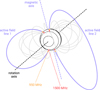 |
Fig. 1 Magnetic field geometry inferred for the T8 dwarf J0623. The dashed lines on the surface are lines of constant latitude in 30° intervals, with the solid line showing the equator. Dipolar field lines with a size of 3 radii are shown in grey, and the two active field lines which emit electron cyclotron maser emission are shown in purple. The emission points at 950 and 1500 MHz are marked on each active field line. The rotation and magnetic axes are also shown as straight dashed lines. The observer’s line of sight is effectively parallel to the rotation axis. The brown dwarf has a large magnetic obliquity, reminiscent of Uranus and Neptune. The active field lines are shown here with their minimum size (see Section 5.1). |
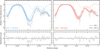 |
Fig. 2 Best fit to the MeerKAT data of JO623 from 950 to 1150 MHz (top left) and 1300 to 1500 MHz (top right). 1σ error bars are shown for each data point. The solid curves and shaded regions show the average and 3σ variance of the model lightcurve over each band. The dotted and dashed curves illustrate the averaged individual contributions of each active field line to the lightcurve. The lower panels show the residuals of the data with the average lightcurve (observed minus model flux density). |
4 Potential magnetic field evolution
J0623 was also observed with the Australian Telescope Compact Array (ATCA) for 6 hours on 14 Aug. 2022 and for 11 hours on 16 Dec. 2022 (Rose et al. 2023). While these observations predate the MeerKAT observations which were taken in Mar. 2023, they have a lower signal to noise ratio in Stokes V. This was our main motivation to primarily analyse the MeerKAT data over the ATCA data. However, it is interesting to explore how our predicted field geometry for J0623 holds up at these other epochs, and determine if there is any evolution in the properties inferred.
Firstly, we reprocessed the ATCA data presented by Rose et al. (2023) to produce the Stokes V lightcurves at different frequency bands. This is described in more detail in Appendix B.2.
For the Aug. data, we obtained two lightcurves from 1.3 to 1.77 GHz and 1.77 to 2.43 GHz. From 2.43 to 3.1 GHz, there is no signal visible. We therefore use this upper band to estimate the noise, which we measure to be 0.34 mJy. Similarly for the Dec. data, we created lightcurves from 1.3 to 1.6 GHz and 1.6 to 2.1 GHz. The band from 2.1 to 3.1 GHz shows no signal, from which we extract a noise value of 0.33 mJy.
The ATCA data show similar structure overall to the MeerKAT data, but some differences become noticeable for the Aug. 14 data in particular. We show a comparison of the MeerKAT and ATCA lightcurves in Figure 4. To explore if this change may pertain to a change in the underlying physical parameters modelled here, we re-apply the same sampling method as for the MeerKAT data. We first allowed only the 2 AFL parameters to vary, fixing the other parameters to those that give maximum likelihood for the MeerKAT data. We then ran an additional test for each epoch allowing the magnetic obliquity to also vary. The results are listed in Table 2. We also show the fits to the data in Figure C.1. For the Dec. data, which were taken closer to the MeerKAT data, we find that the Bayesian evidence is higher if the magnetic obliquity remains unchanged from that inferred for the MeerKAT data. The values inferred also imply a slight change in parameters corresponding to the second AFL.
For the Aug. data on the other hand, the evidence favours a magnetic obliquity of ~50º. The increase in log 𝒵 compared to the case where the other parameters are kept fixed is ~6. However, the reduced χ2 for the fits become worse for the noise and low frequency band when compared to the case where β is fixed as the value inferred from the MeerKAT data. The favoured results here also imply changes in the AFL properties. In particular, they imply that the 2nd AFL has drifted by about 20º in longitude.
These results imply that the magnetic axis has drifted by ~30º over the course of 6 months. Obtaining follow-up data of J0623 with MeerKAT is worth pursuing to explore this further, in that it could allow us to track a potential magnetic cycle on a brown dwarf for the first time. So far, evidence of magnetic cycles past the sub-stellar boundary have only been loosely inferred via changes in the magnetic polarity of radio bursts (Route 2016). Additionally, tracking potential drifts in the positions of the AFLs may allude to the orbital motion of a satellite within the magnetosphere. However, this is purely speculative at this time.
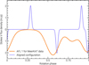 |
Fig. 3 Comparison of the lightcurve of AFL 1 inferred from the MeerKAT data (orange) versus the scenario where JO623 is viewed equator-on with a magnetic obliquity of zero in an ‘aligned’ configuration (purple). In the aligned scenario, the visibility of the emission decreases significantly. Our inferred geometry therefore may hint at a detection bias at radio wavelengths for brown dwarfs in pole-on configurations with large magnetic obliquities. |
Inferred parameters obtained for J0623 assuming 1 or 2 AFLs emit in its large-scale magnetosphere.
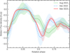 |
Fig. 4 Comparison of the Stokes V lightcurves of J0623 on obtained with ATCA on 14 Aug. 2022 (1.3 – 1.77 GHz) and 16 Dec. 2022 (1.3 – 1.6 GHz), and with MeerKAT on 27 Mar. 2023 (1.3 – 1.5 GHz). For clarity, we linearly resampled the data using 500 uniformly-spaced points in rotation phase, and smoothed the result with a Gaussian with a width of 5σ using SciPy’s gaussian_filterld function. The shaded regions show the 1σ variance in the Stokes V flux density. The structure appears to change over a timescale of around 6 months, which we speculate could be due to a magnetic cycle (see Section 4). |
5 The magnetic field strength of J0623
5.1 Constraints from radio modelling
It is important to note that our inversion method does not depend on the field strength at the magnetic poles B0 (see Appendix C.2). Instead, it depends on the quantity B0/L3, where L is the maximum extent of the AFL in the magnetic equator or ‘loop size’. Equation (C.4) relates B0/L3 to the co-latitude of the emission point θB and the frequency of emission ν. While we cannot break the degeneracy between B0 and L, we can still place constraints on their values.
The first constraint we can place is on the minimum size of L. For emission to be visible, the maximum frequency has to occur above the point where the AFL meets the surface. From Equation (C.3), this requires that
 (2)
(2)
where R is the radius. Since we obtain the co-latitude of the emission point on each co-latitude separately, each AFL has its own minimum size. For the favoured 2 AFL scenario inferred from the MeerKAT data (Table 1), the minimum loop sizes of AFLs 1 and 2 are 4.67 and 10.2 R (as shown in Figure 1). Similarly, for our fits to the 2 ATCA epochs, we estimate minimum loop sizes for AFLs 1 and 2 of 2.37 and 2.65 R in Aug, and 6.51 and 8.21 R in Dec.
The minimum loop sizes also allow us to place a lower limit on the magnetic field strength. This is an important quantity to determine, in that it can inform us about the internal dynamo (Kao et al. 2016). Given the minimum loop size, one can show via Equation (C.4) that
 (3)
(3)
Again, both AFLs provide a constraint on this. However, the constraint provided by the larger magnetic co-latitude should be adopted, in that it provides the largest lower limit, which is required for emission from both AFLs to be visible. From the MeerKAT data, we estimate a lower limit of 585 G on the dipolar field strength of J0623. For the ATCA data on the other hand, we estimate a lower limit of 1339 G in Aug. and 1177 G in Dec. These are significantly larger than the estimate from the MeerKAT data as we predict emission up to 3.1 GHz, albeit at a level that is generally below the noise in the ATCA data (see Figure C.1). While the higher observing band is likely the primary factor for the larger field strength estimates, an increase in the minimum field strength towards the Aug. 2022 epoch may also support the idea for a magnetic cycle as discussed in Section 4.
The method deployed here provides a more robust constraint on magnetic field strengths compared to previous works, in that it is informed by the magnetic co-latitude of the emission cone. In the absence of this information, one has to assume that the emission comes from the magnetic pole (e.g. Kao et al. 2018). Lacking this information, our estimated lower limit from the MeerKAT data would instead be 536 G. We also note that we assume the emission occurs at the fundamental of the cyclotron frequency. However, emission at the first harmonic is also possible, in which case our lower limit here should be halved.
5.2 Comparison to scaling laws
It is also worth comparing our field strength estimates for J0623 to that predicted by the scaling law presented by Christensen et al. (2009). This scaling law gives a prescription for the dipolar field strength as a function of the mass M, luminosity L, and radius R (Reiners et al. 2009; Reiners & Christensen 2010):
 (4)
(4)
Note that all quantities here are in solar units, and MJup is the mass of Jupiter.
To estimate the mass, luminosity, and radius of J0623, we use version 2 of the solar metallicity Sonora Diamondback2 evolutionary models presented by Morley et al. (2024) for UCDs. These provide the effective temperature Teff, surface gravity log 𝑔, and luminosity as a function of age for a given mass. These quantities vary over time, as UCDs expand and cool down via the burning of deuterium. While Morley et al. (2024) also present models that include the effects of atmospheric clouds, we choose to use the cloud-free models as Morley et al. (2024) states that these better-reproduce the measured photometry of T dwarfs (which J0623 is identified as).
To obtain the quantities needed for Equation (4), we need some input quantity to interpolate with between the different evolutionary tracks. For this, we use the estimated values of Teff and log 𝑔 for J0623 obtained by Zhang et al. (2021) from modelling its low-resolution near-infrared spectrum. These are  K and log
  . We note that these values are co-variant. For each set of log 𝑔 and Teff, we linearly interpolate between the values for the mass, radius, and luminosity from the evolutionary tracks using SciPy’s LinearNDInterpolator function. We note that the samples for Teff and log g from Zhang et al. (2021) have a 93% overlap with the evolutionary tracks from Morley et al. (2024). Those that lie outside the bounds of the tracks are discarded.
Interpolating between the evolutionary tracks, we obtain the following estimates for the properties of  , R = 1.01 ± 0.14 RJup, and
  . Plugging these values into Equation (4), we estimate a dipolar field strength of
  G for J0623. For simplicity, we sample the coefficient at the front of Equation (4) from a Gaussian centred at 3.4 kG with a standard deviation of 2.2 kG, as we do not have access to the distribution of its value.
Comparing the estimated dipolar field strength of J0623 to the minimum values estimated in Section 5.1, the value of 341 G is significantly lower. This same result was previously reported by Kao et al. (2018) for other T dwarfs. One way to reconcile this discrepancy is that the emission is in fact coming from small loops associated active regions (e.g. Lynch et al. 2015). However, modelling each AFL with its own magnetic axis introduces more free parameters, which we do not account for in this work. Additionally, the ability for brown dwarfs to sustain such active regions over a significant length of time is uncertain, as pointed out by Kao et al. (2018). Alternatively, it may also occur at the harmonic of the local cyclotron frequency, which would half the field strength estimate. We again note that our method provides a larger lower limit compared to previous works, as it is informed by the magnetic co-latitude of the emission cone. This may cause further deviations from the scaling law proposed by Christensen et al. (2009) if applied to other radio-detected UCDs.
6 Potential plasma sources for J0623
The source of plasma powering both coherent and incoherent radio emission from the magnetospheres of isolated UCDs remains a major open question. One option is that it is driven by a sub-stellar wind. Leto et al. (2021) proposed a mechanism dubbed ‘centrifugal breakout’ (CBO), in which material driven by a wind outflow builds up in the equatorial region around the UCD. The centrifugal force pushes this material outwards, but it is held in place by the strong magnetic field. Eventually, the equator reaches a critical mass at which the magnetic field can no longer hold on to the material, and it is flung outwards, snapping open closed field lines in the process. These subsequently reconnect, releasing energy and driving electron acceleration towards the magnetic poles. This process is analogous to the co-rotation breakdown mechanism that has been inferred for Jupiter (Zarka 2007; Nichols et al. 2012), which involves interplay between the plasma from both Io and the wind of the Sun (Cowley & Bunce 2001).
Leto et al. (2021) illustrated that the CBO mechanism can reproduce the observed radio luminosities of a few late M-dwarfs and early L-dwarfs. However, it seems less promising for cooler UCDs, given that they do not exhibit any signs of coronae (Williams et al. 2014; Magaudda et al. 2024), which is a key ingredient for driving a wind outflow at low masses (although see the recent work by Walters et al. 2023). Alternatively, orbiting satellites may feed plasma to the magnetosphere via outgassing, analogous to Jupiter’s moon Io (Neubauer 1980). Similar to the CBO mechanism, this material may build up within the equatorial region, which could cause reconnection analogous as described in Section 3.
The co-rotation radius depends on the mass and rotation rate (Jardine & Collier Cameron 2019):
 (5)
(5)
where P is the rotation period. Using the mass and radius estimates for J0623 from Section 5.1, we estimate a small co-rotation radius of  This is unsurprising given its rapid rotation. It is interesting that the co-rotation radius is smaller than the minimum loop size inferred at the 3 epochs where radio emission was observed (Section 5.1). This could resemble a scenario similar to CBO, in that the AFLs would interact with plasma outside of the co-rotation radius. However, it is unclear as to if the timescale for CBO corresponds to the ‘lifetime’ of the bursts seen on J0623. Nevertheless, it is also worth noting that the concept of material forced into co-rotation via the magnetic field is reminiscent of the recent findings by Bouma et al. (2024) indicative of co-rotating clumps of gas around pre-main sequence M dwarfs (referred to as complex periodic variables).
The question also still remains of why only two specific field lines emit within the magnetosphere of J0623. It could be that the field has a shape that is more complex than a dipole, and these lines are simply those that are visible to us. Alternatively, small loops associated with active regions could mimic the signature we infer with the 2 AFLs (Lynch et al. 2015). However, given the stability of the lightcurve between Dec. 2022 and Mar. 2023 (Figure 4), this is difficult to reconcile.
7 Conclusions
In this work, we developed a new tomographic technique for extracting the magnetic properties of objects producing radio emission via the electron cyclotron maser instability. We demonstrate its merit by applying to the ultracool dwarf (UCD) WISE J062309.94-045624.6 (J0623), and infer that it has a dipolar field strength exceeding ~6OO G and a large magnetic obliquity (the angle between its rotation and magnetic axes). Characterising the magnetic fields of UCDs can provide a wealth of information pertaining to their internal composition and dynamo generation. It can also better inform us about the magnetic fields of exo-planets, which to date remain undetected. We also show that our framework can be used to track magnetic cycles on radio-loud systems such as J0623.
It is worth noting that our method could inform signatures of ‘auroral’-like emission on UCDs at other wavelengths. For instance, Hallinan et al. (2015) showed that the M8.5 dwarf LSR J1835+3259 exhibits modulated Hα over the same timescale as its coherent radio bursts. This Hα emission therefore may also be encoded with information about the magnetic field geometry, which could inform our radio modelling and vice versa. Additionally, JWST has begun to uncover emission features indicative of auroral processes on UCDs (e.g. Faherty et al. 2024). These examples highlight the benefit of multi-wavelength observations.
The viewing geometry and magnetic field configuration we infer for J0623 are of particular note, in that Kavanagh & Vedantham (2023) showed that radio surveys are biased towards detecting signatures of magnetic star-planet interactions from systems with the same geometric configuration. Therefore, other radio-detected UCDs may also be in similar configurations. In terms of biases, Kao & Pineda (2024) also recently demonstrated that detection of quiescent radio emission from UCDs is more favourable in binaries. This could also be due to geometric effects, and/or enhanced energetics powering the emission. Whether this also holds for coherent radio emission from UCDs remains to be seen, however our findings may inform this.
In terms of our model, an important aspect it does not capture is propagation effects. Depending on the plasma conditions in the magnetosphere, ECM emission may refract and or be absorbed as it propagates outwards. This will alter the visibility of the emission, which in turn will affect the inferred geometry. However, developing a model that captures these processes which can interface with sampling algorithms efficiently is likely a complex task. Additionally, we currently have little-to-no information about the plasma environments surrounding UCDs. Therefore, these efforts will require additional parame-terisation, further increasing the dimensionality of the problem. We also note there are hints of additional sub-structure within the lightcurves of J0623 that our model does not capture. These could be due to a field that is more complex than our assumed dipolar field shape, which could include smaller-scale surface features as inferred on other UCDs (Lynch et al. 2015). Accounting for more complex fields will also increase the dimensionality of the problem. However, this is worth exploring further from an inversion perspective, which may rule out the large-scale dipolar magnetic field we infer here.
Acknowledgements
RDK, HKV, and SB acknowledge funding from the Dutch Research Council (NWO) for the project ‘e-MAPS’ (project number Vi.Vidi.203.093) under the NWO talent scheme VIDI. HKV also acknowledges funding from the European Research Council for the project ‘Stormchaser’ (grant number 101042416). KR acknowledges the LSST-DA Data Science Fellowship Program, which is funded by LSST-DA, the Brinson Foundation, and the Moore Foundation; Their participation in the program has benefited this work. The MeerKAT telescope is operated by the South African Radio Astronomy Observatory, which is a facility of the National Research Foundation, an agency of the Department of Science and Innovation. The Australia Telescope Compact Array is part of the Australia Telescope National Facility, which is funded by the Australian Government for operation as a National Facility managed by CSIRO. We acknowledge the Gomeroi people as the Traditional Owners of the Observatory site. We thank Dr Zhoujian Zhang for providing their sampling chains from Zhang et al. (2021) for the effective temperature and surface gravity of J0623, which were used to estimate its mass, radius, and luminosity. We also thank Dr Joe Callingham for sharing their comments and suggestions on the manuscript. Software: NumPy (Harris et al. 2020), SciPy (Virtanen et al. 2020), pandas (The Pandas Development Team 2020), Matplotlib (Hunter 2007), corner (Foreman-Mackey 2016), UltraNest (Buchner 2016, 2019, 2021).
Appendix A ECM emission from active field lines
A.1 Precession of the magnetic axis
The visibility of ECM emission as a function of time depends on the orientation of the magnetic axis  relative to the line of sight and the longitude of the AFL ϕB. It is convenient to define the coordinates relative to the line of sight, which we do as follows. The line of sight
  points from the centre of the object to the observer. We note that vectors denoted with a hat are unit vectors. The rotation axis
  is inclined relative to
  by the angle i:
 (A.1)
(A.1)
where  is the projection of
  on to the plane of the sky.
  then completes the vector basis for the coordinate system.
We trace the rotation with the vector  . First, we project
  onto the equatorial plane, which is
 (A.2)
(A.2)
 is measured from this vector, with which it forms the rotation phase angle
 (A.3)
(A.3)
i.e.
 (A.4)
(A.4)
In other words, the rotation phase is zero when  . Additionally, ϕ0 is the rotation phase at t = 0. We note that a third vector is also required here to complete the basis describing the rotation:
 (A.5)
(A.5)
The plane defined by  and
and  contains the magnetic axis
  , which is inclined relative to
  by the magnetic obliquity β:
 (A.6)
(A.6)
When β ≠ 0 or 180°, the observer will see  precess about the rotation axis. It is also convenient to project
  on to the magnetic equator:
 (A.7)
(A.7)
This provides a reference vector to measure the magnetic longitude ϕB from for each AFL:
 (A.8)
(A.8)
i.e. this vector locates the AFL in the magnetic equator. See Figure A.1 for a graphical illustration of the coordinate system described here.
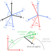 |
Fig. A.1 Sketch of the coordinate system adopted to calculate the visibility of ECM emission from the active field lines. The top left vectors show the relation between the line of sight and rotation coordinates, and the top right vectors show the relation between the rotation and magnetic vectors. The bottom panel shows the vectors that define the plane containing active field line, which emits in a hollow cone configuration centred on the vector ĉ, which has an opening angle α. The visibility of the ECM emission is dependent on the angle γ formed between ĉ and the line of sight |

A.2 Beam angle
The plane formed by the vectors  and
and  contains the AFL, which is dipolar in shape. The unit vector ĉ at each point on the field line, which is the normalised magnetic field vector, is (Bloot et al. 2024):
 (A.9)
(A.9)
where θB is the magnetic co-latitude of the point measured from  , and
, and
 (A.10)
 (A.11)
An emission cone on the AFL will be aligned with the vector ĉ. At any frequency, cyclotron emission can occur at two points on the AFL, one in each magnetic hemisphere. The line is symmetric, meaning that emission at a given frequency and co-latitude θB also occurs at co-latitude π − θB. Hence the ± symbol in Equation A.9, which refers to the Northern and Southern magnetic hemisphere.
The angle ĉ makes with the line of sight determines if emission is visible to the observer. We obtain this by taking the dot product:
 (A.12)
Expanding the dot product terms above gives the following:
 (A.13)
 (A.14)
where
 (A.15)
 (A.16)
 (A.17)
 (A.18)
 (A.19)
Rewriting Equation A.12, we have
 (A.20)
Expanding the terms sin ϕrot and cos ϕrot then gives the following expressions for the beam angle from the Northern and Southern hemispheres:
 (A.21)
 (A.22)
where
 (A.23)
 (A.24)
 (A.25)
 (A.26)
 (A.27)
 (A.28)
Note that the model lightcurve does not depend on the emission frequency (see Appendix C.2). Additionally, some of the parameters Equation A.12 depends on are degenerate, which we describe in Appendix A.3.
A.3 Degeneracies
Given that the forward model presented here is predominantly geometric, it is important to identify degeneracies it contains to aid the convergence of the sampling algorithm utilised. The degeneracies we identify are due to symmetries in the functions used to model the beam angle from each hemisphere. For instance, if one replaces i with π − i, β with π − β, and ϕB with π – ϕB, the functional forms of Equations A.21 and A.22 are unchanged.
An additional symmetry can be found in the expressions for a and b (Equations A.10 and A.11). For θB ∈ [0, π/2], there are two values of θB that give the same value of a. These are given by
 (A.29)
which lie either side of the maximum of a which occurs at  . So, swapping θB for the other solution to Equation A.29 gives the same value for a. Additionally, a2 + b2 = 1, so the value of b is inverted for the second value of θB. If the value of θB is swapped in this case, the following transformations can be made to retain the function forms of Equations A.21 and A.22:
i → π − i, ϕ0 → π + ϕ0, ϕB → π + ϕB
β → π − β, ϕ0 → π + ϕ0, ϕB → 2π − ϕB
In order to avoid these degeneracies, we limit the range of values for i and β from 0 to 90º. In other words, our inferred values for i and β cannot be distinguished between their supplementary angles. Therefore, we cannot tell the direction of rotation of the pole we see, nor the polarity of the magnetic pole we see. The latter is further obscured by the fact that we do not know the magnetoionic mode under which the ECM emission is operating for J0623, which will flip the sign of the circularly polarised flux density measured from a region of a given magnetic polarity (Kavanagh et al. 2022).
Appendix B Data reduction
B.1 MeerKAT
The MeerKAT data presented by Rose et al. (2023) shows slight differences in structure from 950 to 1150 MHz and 1300 to 1500 MHz. To account for this in our sampling method, we took the 64 second time-averaged data from Rose et al. (2023) and created two lightcurves averaged over the 950–1150 MHz and 1300–1500 MHz frequency sub-bands, respectively. The uncertainties for each flux density measurement are the standard error obtained by computing the standard deviation of the imaginary component of the emission across the frequency sub-band and normalising by the square root of the number of channels in that band. We then replace any missing values across the observation with the arithmetic mean of these standard error uncertainties.
We then phase folded the two lightcurves using the rotation period inferred by Rose et al. (2023) of 1.912 hours. From rotation to rotation, the structure in the lightcurves shows some variation. This is particularly noticeable in the first burst in the high frequency band (see Figure 2 of Rose et al. 2023). However, our model assumes a fixed flux density for each AFL. To account for these intrinsic variations, we first define bins in phase space, each with a width equal to the time resolution of the MeerKAT data divided by the rotation phase. Then, we resample the points in each phase bin from a Gaussian distribution 10 000 times. We then compute the average value and standard deviation of all the resampled points in each bin. As a result, the error in phase for each bin contains both the measurement error for each point and the intrinsic variations from rotation to rotation. With the data formatted, we can then compute the likelihood function for UltraNest to sample.
B.2 ATCA
J0623 was observed with ATCA twice in 2022 (Project ID: C3363, PI: T Murphy), at 1.1 to 3.1 GHz using the 2 GHz Compact Array Broadband Backend (CABB, Wilson et al. 2011). The first observation was taken on 2022-08-14, in the H168 configuration, with an observing time of 6 h. The second observation lasted for 11 hours and was taken in the 6D configuration.
We reduced the data using casa version 6.4 (CASA Team 2022). The data was flagged using the tfcrop algorithm, resulting in on average 50–60% of the data being flagged. We use PKS B1934-638 as the flux density and bandpass calibrator, and J0607-157 as the phase calibrator. PKS B1934-638 was observed for 10 minutes at the start of each observation. The phase calibrator was observed for 2 minutes after every 20 minutes on target.
We first determined the gain, bandpass, polarisation and polarisation leakage solutions on the flux density calibrator, using a solution interval of 60 s. After transferring these solutions to the phase calibrator, we use the qufromgain task from the atca.polhelpers package for linear polarisation calibration. The combined solutions were then transferred to the target.
For both epochs, we create Stokes V light curves of either 3 or 4 frequency bins as described in Section 4, using the method described in Bloot et al. (2024). We define the sign of Stokes V as right-handed circularly polarised emission minus left-handed circular polarised emission, in agreement with the IAU convention (Hamaker & Bregman 1996). We then phase-folded and binned the data in the same manner as for the MeerKAT data.
Appendix C Parameter space exploration with UltraNest
C.1 Computing the likelihood function
The main component of running a sampling algorithm such as UltraNest is setting up the likelihood and posterior functions. In the case of the 2 MeerKAT bands, the lightcurves show little variation in frequency. To account for this in our likelihood function, we compute the model lightcurve Fν for 8 frequencies spaced uniformly over each band via Equation 1. We then compute the total log likelihood by summing up the log likelihood of each model lightcurve with its respective band of observed emission Fobs:
 (C.1)
(C.1)
where σobs is the standard deviation in each phase bin, which is computed as described in Appendix B.1. Computing the model lightcurve Fν requires the magnetic co-latitude of emission at each frequency (Appendix A.2). We describe our method for calculating this in Appendix C.2.
C.2 The magnetic co-latitude of a given frequency
Our lightcurve model does not depend on the emitted frequency (Appendix A.2). Instead, it depends on the magnetic co-latitude of the emitting point θB. The magnetic field strength on a dipolar field line is (Kivelson & Russell 1995):
 (C.2)
(C.2)
where B0 is the field strength at the magnetic poles, R is the radius, and r is the radial distance to the emitting point from the centre. The coordinates on a dipolar field line also relate to one another via:
 (C.3)
(C.3)
where L is the loop size measured from the centre to its maximum extent in the magnetic equator. Additionally, fundamental cyclotron emission occurs at a frequency of ν = 2.8 B MHz, where B is in Gauss. Combining all this together, one can show that
 (C.4)
(C.4)
Our sampling routine provides us with the value of θB that best-reproduces the observed lightcurve. Assigning the frequency of emission ν at this magnetic co-latitude therefore means that the left-hand side of Equation C.4 is constant. In other words, one can increase both the dipolar field strength and loop size without changing the lightcurve morphology.
In our sampling routine, we first draw the co-latitude θmax corresponding to the maximum frequency νmax. Since Equation C.4 is constant for each AFL, we can write an expression relating the co-latitude at νmax to the co-latitude θB corresponding to emission at any frequency ν:
 (C.5)
(C.5)
Rewriting, we have:
 (C.6)
(C.6)
where
 (C.7)
(C.7)
 (C.8)
(C.8)
 (C.9)
(C.9)
To solve Equation C.6, we use Newton’s method, i.e.:
 (C.10)
Initialising the value of xi = xmax, the relative difference between the left and right-hand side of Equation C.5 becomes less than 10−10 within 5 iterations. We solve Equation C.10 for each of the 8 uniformly spaced frequencies over the observed band. We note that this is done independently for each AFL. With the co-latitude at each frequency obtained, we can then compute the likelihood via Equation C.1.
C.3 Adopted priors for the parameter space
We also must specify the priors each model parameter. The full list of parameters is as follows:
The inclination of the rotation axis i.
The magnetic obliquity β.
The rotation phase at the start of the MeerKAT observations ϕ0.
The emission cone opening angle α and thickness ∆α.
The magnetic co-latitude of the emission site on each AFL (θ1, θ2,…).
The longitude of the AFL in the magnetic equator (ϕ1,ϕ2,…).
The flux density measured from each AFL when the beam direction is aligned exactly with the line of sight (F1, F2,…).
We have little information about any of these quantities, so we adopt uniform priors for each. We note that for the inclination i, we uniformly sample cos i (see Kavanagh & Vedantham 2023). The inclination and magnetic obliquity are also constrained by the degeneracies as described in Appendix A.3. On Jupiter, opening angles of around 70 to 80° and thicknesses of a few degrees are inferred from in-situ observations (Kaiser et al. 2000; Louis et al. 2023), although theoretical models suggest that lower opening angles are also possible (Stupp 2000). Given the uncertainties and complexities leading to the resulting cone parameters of ECM emission, we choose to vary the opening angle from 0 to 90 degrees, and consider thicknesses up to 10 degrees.
Another constraint to note is on the max value of the co-latitude of the emission cone. In our sampling routine, our input value is the co-latitude at the maximum frequency νmax. However, if the co-latitude is too large, it will not be possible to generate emission on the AFL at the lowest frequency νmin. To avoid this, we limit the value of θB at νmax to be less the value which places emission at νmin. Rewriting Equation C.5, we have
 (C.11)
where νmin = 950 MHz and νmax = 1500 MHz for the MeerKAT data, and νmin = 1.3 GHz and νmax = 3.1 GHz for the ATCA data. Setting θmin = 90º, we solve Equation C.11 as described in Appendix C.2. For the MeerKAT data, we obtain θmax = 71.36º, and for the ATCA data θmax = 63.98º.
List of the priors adopted for each parameter in our model.
For the flux density of each AFL, we set the minimum value to be 1 mJy, which is the lowest burst flux seen in the MeerKAT data. The upper limit of 10 mJy is chosen to allow the sampler to also explore scenarios where significant flux cancellation occurs between emission cones in the two magnetic hemispheres. The remaining parameters are self explanatory, i.e. the initial phase and magnetic longitude of each AFL are uniformly sampled in on a circle. We also note that we enforce the value of ϕB for AFL 2 to be greater than that for AFL 1. Table C.1 lists all of the priors.
C.4 Running the sampler
With the likelihood and prior functions set up, we then use UltraNest’s step sampler function SliceSampler, which is recommended for efficient sampling in high dimensions3. For the generate_direction parameter of SliceSampler, we use generate_mixture_random_direction, which performs best in high dimensional spaces (Buchner 2022). For each dataset and number of AFLs, we run the sampler multiple times and manually check if it converges on the same result. If the results are inconsistent, we double the number of steps the sampler takes via the nsteps parameter. For the MeerKAT data, the sampler converges in 200 steps for 1 AFL and 400 steps for 2 AFLs, whereas for the ATCA data it converges in 100 steps for both 1 and 2 AFLs. Our best fits to the MeerKAT and ATCA data are shown in Figures 2 and C.1. We also show the converged posterior distributions for the MeerKAT and ATCA data in Figures C.2 and C.3. An example script showing our setup for sampling the likelihood space defined by our model can be found on GitHub4.
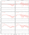 |
Fig. C.1 Same as Figure 2 except for the best fit to the Aug and Dec. ATCA data. The parameters inferred at these two epochs are listed in Table 2. The top panels show the 1σ ‘noise’ bands in which we do not find any significant emission. The rotation phases shown here are consistent with those in Figure 2. |
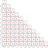 |
Fig. C.2 Posterior distributions of the best-fitting model parameters listed in Table 1 plotted using corner (Foreman-Mackey 2016). The shaded regions in each panel bar the diagonal ones show the 16th, 50th, and 84th percentiles going from darkest to lightest in colour. We have smoothed the contours by setting the smooth parameter to 1 in the corner function to better-highlight the 16th percentile region. The diagonal panels show the flattened histogram for each parameter (unsmoothed). |
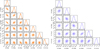 |
Fig. C.3 Same as Figure C.2 except for the Aug (left) and Dec (right) ATCA data. The derived confidence intervals for each parameter are listed in Table 2. Dec data favours the magnetic magnetic obliquity β to be fixed as the value inferred from the MeerKAT data. |
References
- Bagenal, F. 2013, in Planets, Stars and Stellar Systems, 3: Solar and Stellar Planetary Systems, eds. T. D. Oswalt, L. M. French, & P. Kalas, 251 [CrossRef] [Google Scholar]
- Bastian, T. S., Cotton, W. D., & Hallinan, G. 2022, ApJ, 935, 99 [NASA ADS] [CrossRef] [Google Scholar]
- Behmard, A., Petigura, E. A., & Howard, A. W. 2019, ApJ, 876, 68 [NASA ADS] [CrossRef] [Google Scholar]
- Berdyugina, S. V., Harrington, D. M., Kuzmychov, O., et al. 2017, ApJ, 847, 61 [NASA ADS] [CrossRef] [Google Scholar]
- Berger, E., Ball, S., Becker, K. M., et al. 2001, Nature, 410, 338 [NASA ADS] [CrossRef] [Google Scholar]
- Bloot, S., Callingham, J. R., Vedantham, H. K., et al. 2024, A&A, 682, A170 [NASA ADS] [CrossRef] [EDP Sciences] [Google Scholar]
- Bouma, L. G., Jayaraman, R., Rappaport, S., et al. 2024, AJ, 167, 38 [NASA ADS] [CrossRef] [Google Scholar]
- Braun, R., Bonaldi, A., Bourke, T., Keane, E. F., & Wagg, J. 2017, Anticipated SKA1 Science Performance, SKA-TEL-SKO-0000818 [Google Scholar]
- Buchner, J. 2016, Statist. Comput., 26, 383 [NASA ADS] [CrossRef] [Google Scholar]
- Buchner, J. 2019, PASP, 131, 108005 [Google Scholar]
- Buchner, J. 2021, J. Open Source Softw., 6, 3001 [CrossRef] [Google Scholar]
- Buchner, J. 2022, in Physical Sciences Forum, 5 (Physical Sciences Forum), 46 [NASA ADS] [Google Scholar]
- Callingham, J. R., Gaensler, B. M., Ekers, R. D., et al. 2015, ApJ, 809, 168 [Google Scholar]
- Carolan, S., Vidotto, A. A., Hazra, G., Villarreal D’Angelo, C., & Kubyshkina, D. 2021, MNRAS, 508, 6001 [NASA ADS] [CrossRef] [Google Scholar]
- CASA Team (Bean, B., et al.) 2022, PASP, 134, 114501 [NASA ADS] [CrossRef] [Google Scholar]
- Christensen, U. R., Holzwarth, V., & Reiners, A. 2009, Nature, 457, 167 [Google Scholar]
- Climent, J. B., Guirado, J. C., Pérez-Torres, M., Marcaide, J. M., & Peña-Moñino, L. 2023, Science, 381, 1120 [NASA ADS] [CrossRef] [Google Scholar]
- Cowley, S. W. H., & Bunce, E. J. 2001, Planet. Space Sci., 49, 1067 [NASA ADS] [CrossRef] [Google Scholar]
- Das, B., & Chandra, P. 2021, ApJ, 921, 9 [NASA ADS] [CrossRef] [Google Scholar]
- Donati, J. F., Cristofari, P. I., Finociety, B., et al. 2023, MNRAS, 525, 455 [NASA ADS] [CrossRef] [Google Scholar]
- Dulk, G. A. 1985, ARA&A, 23, 169 [Google Scholar]
- Edler, H. W., de Gasperin, F., & Rafferty, D. 2021, A&A, 652, A37 [NASA ADS] [CrossRef] [EDP Sciences] [Google Scholar]
- Faherty, J. K., Burningham, B., Gagné, J., et al. 2024, Nature, 628, 511 [NASA ADS] [CrossRef] [Google Scholar]
- Foreman-Mackey, D. 2016, J. Open Source Softw., 1, 24 [Google Scholar]
- Hallinan, G., Antonova, A., Doyle, J. G., et al. 2006, ApJ, 653, 690 [NASA ADS] [CrossRef] [Google Scholar]
- Hallinan, G., Bourke, S., Lane, C., et al. 2007, ApJ, 663, L25 [NASA ADS] [CrossRef] [Google Scholar]
- Hallinan, G., Antonova, A., Doyle, J. G., et al. 2008, ApJ, 684, 644 [Google Scholar]
- Hallinan, G., Littlefair, S. P., Cotter, G., et al. 2015, Nature, 523, 568 [NASA ADS] [CrossRef] [Google Scholar]
- Hamaker, J. P., & Bregman, J. D. 1996, A&AS, 117, 161 [NASA ADS] [CrossRef] [EDP Sciences] [Google Scholar]
- Harris, C. R., Millman, K. J., van der Walt, S. J., et al. 2020, Nature, 585, 357 [NASA ADS] [CrossRef] [Google Scholar]
- Herbst, K., Grenfell, J. L., Sinnhuber, M., et al. 2019, A&A, 631, A101 [NASA ADS] [CrossRef] [EDP Sciences] [Google Scholar]
- Hunter, J. D. 2007, Comput. Sci. Eng., 9, 90 [NASA ADS] [CrossRef] [Google Scholar]
- Jardine, M., & Collier Cameron, A. 2019, MNRAS, 482, 2853 [NASA ADS] [CrossRef] [Google Scholar]
- Jasinski, J. M., Murphy, N., Jia, X., & Slavin, J. A. 2022, PSJ, 3, 76 [NASA ADS] [Google Scholar]
- Kaiser, M. L., Zarka, P., Kurth, W. S., Hospodarsky, G. B., & Gurnett, D. A. 2000, J. Geophys. Res., 105, 16053 [NASA ADS] [CrossRef] [Google Scholar]
- Kao, M. M., & Pineda, J. S. 2022, ApJ, 932, 21 [NASA ADS] [CrossRef] [Google Scholar]
- Kao, M. M., & Pineda, J. S. 2024, MNRAS submitted [arXiv:2403.08860] [Google Scholar]
- Kao, M. M., Hallinan, G., Pineda, J. S., et al. 2016, ApJ, 818, 24 [NASA ADS] [CrossRef] [Google Scholar]
- Kao, M. M., Hallinan, G., Pineda, J. S., Stevenson, D., & Burgasser, A. 2018, ApJS, 237, 25 [NASA ADS] [CrossRef] [Google Scholar]
- Kao, M. M., Mioduszewski, A. J., Villadsen, J., & Shkolnik, E. L. 2023, Nature, 619, 272 [NASA ADS] [CrossRef] [Google Scholar]
- Kavanagh, R. D., & Vedantham, H. K. 2023, MNRAS, 524, 6267 [NASA ADS] [CrossRef] [Google Scholar]
- Kavanagh, R. D., Vidotto, A. A., Vedantham, H. K., et al. 2022, MNRAS, 514, 675 [CrossRef] [Google Scholar]
- Kimura, T., & Murakami, M. 2021, PNAS, 118, e2021810118 [NASA ADS] [CrossRef] [Google Scholar]
- Kivelson, M. G., & Russell, C. T. 1995, Introduction to Space Physics [CrossRef] [Google Scholar]
- Knapp, M., Paritsky, L., Kononov, E., & Kao, M. M. 2024, Great Observatory for Long Wavelengths (GO-LoW) NIAC Phase I Final Report, Tech. rep. [Google Scholar]
- Kochukhov, O. 2021, A&A Rev., 29, 1 [NASA ADS] [CrossRef] [Google Scholar]
- Kuzmychov, O., Berdyugina, S. V., & Harrington, D. M. 2017, ApJ, 847, 60 [NASA ADS] [CrossRef] [Google Scholar]
- Leto, P., Trigilio, C., Krticka, J., et al. 2021, MNRAS, 507, 1979 [NASA ADS] [CrossRef] [Google Scholar]
- Llama, J., Jardine, M. M., Wood, K., Hallinan, G., & Morin, J. 2018, ApJ, 854, 7 [Google Scholar]
- Louis, C. K., Louarn, P., Collet, B., et al. 2023, J. Geophys. Res. (Space Phys.), 128, e2023JA031985 [NASA ADS] [CrossRef] [Google Scholar]
- Lynch, C., Mutel, R. L., & Güdel, M. 2015, ApJ, 802, 106 [NASA ADS] [CrossRef] [Google Scholar]
- Magaudda, E., Stelzer, B., Osten, R. A., et al. 2024, A&A, 687, A95 [NASA ADS] [CrossRef] [EDP Sciences] [Google Scholar]
- Marques, M. S., Zarka, P., Echer, E., et al. 2017, A&A, 604, A17 [NASA ADS] [CrossRef] [EDP Sciences] [Google Scholar]
- McConnell, D., Hale, C. L., Lenc, E., et al. 2020, PASA, 37, e048 [Google Scholar]
- Melrose, D. B., & Dulk, G. A. 1982, ApJ, 259, 844 [Google Scholar]
- Morley, C. V., Mukherjee, S., Marley, M. S., et al. 2024, ApJ, 975, 59 [NASA ADS] [CrossRef] [Google Scholar]
- Neubauer, F. M. 1980, J. Geophys. Res., 85, 1171 [Google Scholar]
- Nichols, J. D., Burleigh, M. R., Casewell, S. L., et al. 2012, ApJ, 760, 59 [Google Scholar]
- Owen, J. E., & Adams, F. C. 2014, MNRAS, 444, 3761 [Google Scholar]
- Reiners, A., & Christensen, U. R. 2010, A&A, 522, A13 [NASA ADS] [CrossRef] [EDP Sciences] [Google Scholar]
- Reiners, A., Basri, G., & Christensen, U. R. 2009, ApJ, 697, 373 [NASA ADS] [CrossRef] [Google Scholar]
- Richey-Yowell, T., Kao, M. M., Pineda, J. S., Shkolnik, E. L., & Hallinan, G. 2020, ApJ, 903, 74 [NASA ADS] [CrossRef] [Google Scholar]
- Rodríguez-Mozos, J. M., & Moya, A. 2022, A&A, 661, A101 [NASA ADS] [CrossRef] [EDP Sciences] [Google Scholar]
- Rodgers-Lee, D., Rimmer, P. B., Vidotto, A. A., et al. 2023, MNRAS, 521, 5880 [NASA ADS] [CrossRef] [Google Scholar]
- Rose, K., Pritchard, J., Murphy, T., et al. 2023, ApJ, 951, L43 [NASA ADS] [CrossRef] [Google Scholar]
- Route, M. 2016, ApJ, 830, L27 [CrossRef] [Google Scholar]
- Shultz, M. E., Owocki, S. P., ud-Doula, A., et al. 2022, MNRAS, 513, 1429 [NASA ADS] [CrossRef] [Google Scholar]
- Stupp, A. 2000, MNRAS, 311, 251 [CrossRef] [Google Scholar]
- Tang, J., Tsai, C.-W., & Li, D. 2022, Res. Astron. Astrophys., 22, 065013 [CrossRef] [Google Scholar]
- Tannock, M. E., Metchev, S., Heinze, A., et al. 2021, AJ, 161, 224 [NASA ADS] [CrossRef] [Google Scholar]
- The Pandas Development Team. 2020, pandas-dev/pandas: Pandas, https://doi.org/10.5281/zenodo.3509134 [Google Scholar]
- Treumann, R. A. 2006, A&A Rev., 13, 229 [NASA ADS] [CrossRef] [Google Scholar]
- Turner, J. D., Zarka, P., Grießmeier, J.-M., et al. 2021, A&A, 645, A59 [NASA ADS] [CrossRef] [EDP Sciences] [Google Scholar]
- Turner, J. D., Grießmeier, J.-M., Zarka, P., Zhang, X., & Mauduit, E. 2024, A&A, 688, A66 [NASA ADS] [CrossRef] [EDP Sciences] [Google Scholar]
- Vedantham, H. K., Callingham, J. R., Shimwell, T. W., et al. 2020, ApJ, 903, L33 [Google Scholar]
- Vedantham, H. K., Dupuy, T. J., Evans, E. L., et al. 2023, A&A, 675, L6 [NASA ADS] [CrossRef] [EDP Sciences] [Google Scholar]
- Virtanen, P., Gommers, R., Oliphant, T. E., et al. 2020, Nat. Methods, 17, 261 [Google Scholar]
- Walters, N., Farihi, J., Dufour, P., Pineda, J. S., & Izzard, R. G. 2023, MNRAS, 524, 5096 [CrossRef] [Google Scholar]
- Williams, P. K. G. 2018, in Handbook of Exoplanets, eds. H. J. Deeg, & J. A. Belmonte, 171 [Google Scholar]
- Williams, P. K. G., Cook, B. A., & Berger, E. 2014, ApJ, 785, 9 [Google Scholar]
- Wilson, W. E., Ferris, R. H., Axtens, P., et al. 2011, MNRAS, 416, 832 [Google Scholar]
- Zarka, P. 2007, Planet. Space Sci., 55, 598 [Google Scholar]
- Zhang, Z., Liu, M. C., Marley, M. S., Line, M. R., & Best, W. M. J. 2021, ApJ, 921, 95 [NASA ADS] [CrossRef] [Google Scholar]
All Tables
Inferred parameters obtained for J0623 assuming 1 or 2 AFLs emit in its large-scale magnetosphere.
All Figures
|
Fig. 1 Magnetic field geometry inferred for the T8 dwarf J0623. The dashed lines on the surface are lines of constant latitude in 30° intervals, with the solid line showing the equator. Dipolar field lines with a size of 3 radii are shown in grey, and the two active field lines which emit electron cyclotron maser emission are shown in purple. The emission points at 950 and 1500 MHz are marked on each active field line. The rotation and magnetic axes are also shown as straight dashed lines. The observer’s line of sight is effectively parallel to the rotation axis. The brown dwarf has a large magnetic obliquity, reminiscent of Uranus and Neptune. The active field lines are shown here with their minimum size (see Section 5.1). |
| In the text | |
|
Fig. 2 Best fit to the MeerKAT data of JO623 from 950 to 1150 MHz (top left) and 1300 to 1500 MHz (top right). 1σ error bars are shown for each data point. The solid curves and shaded regions show the average and 3σ variance of the model lightcurve over each band. The dotted and dashed curves illustrate the averaged individual contributions of each active field line to the lightcurve. The lower panels show the residuals of the data with the average lightcurve (observed minus model flux density). |
| In the text | |
|
Fig. 3 Comparison of the lightcurve of AFL 1 inferred from the MeerKAT data (orange) versus the scenario where JO623 is viewed equator-on with a magnetic obliquity of zero in an ‘aligned’ configuration (purple). In the aligned scenario, the visibility of the emission decreases significantly. Our inferred geometry therefore may hint at a detection bias at radio wavelengths for brown dwarfs in pole-on configurations with large magnetic obliquities. |
| In the text | |
|
Fig. 4 Comparison of the Stokes V lightcurves of J0623 on obtained with ATCA on 14 Aug. 2022 (1.3 – 1.77 GHz) and 16 Dec. 2022 (1.3 – 1.6 GHz), and with MeerKAT on 27 Mar. 2023 (1.3 – 1.5 GHz). For clarity, we linearly resampled the data using 500 uniformly-spaced points in rotation phase, and smoothed the result with a Gaussian with a width of 5σ using SciPy’s gaussian_filterld function. The shaded regions show the 1σ variance in the Stokes V flux density. The structure appears to change over a timescale of around 6 months, which we speculate could be due to a magnetic cycle (see Section 4). |
| In the text | |
|
Fig. A.1 Sketch of the coordinate system adopted to calculate the visibility of ECM emission from the active field lines. The top left vectors show the relation between the line of sight and rotation coordinates, and the top right vectors show the relation between the rotation and magnetic vectors. The bottom panel shows the vectors that define the plane containing active field line, which emits in a hollow cone configuration centred on the vector ĉ, which has an opening angle α. The visibility of the ECM emission is dependent on the angle γ formed between ĉ and the line of sight |
| In the text | |
|
Fig. C.1 Same as Figure 2 except for the best fit to the Aug and Dec. ATCA data. The parameters inferred at these two epochs are listed in Table 2. The top panels show the 1σ ‘noise’ bands in which we do not find any significant emission. The rotation phases shown here are consistent with those in Figure 2. |
| In the text | |
|
Fig. C.2 Posterior distributions of the best-fitting model parameters listed in Table 1 plotted using corner (Foreman-Mackey 2016). The shaded regions in each panel bar the diagonal ones show the 16th, 50th, and 84th percentiles going from darkest to lightest in colour. We have smoothed the contours by setting the smooth parameter to 1 in the corner function to better-highlight the 16th percentile region. The diagonal panels show the flattened histogram for each parameter (unsmoothed). |
| In the text | |
|
Fig. C.3 Same as Figure C.2 except for the Aug (left) and Dec (right) ATCA data. The derived confidence intervals for each parameter are listed in Table 2. Dec data favours the magnetic magnetic obliquity β to be fixed as the value inferred from the MeerKAT data. |
| In the text | |
Current usage metrics show cumulative count of Article Views (full-text article views including HTML views, PDF and ePub downloads, according to the available data) and Abstracts Views on Vision4Press platform.
Data correspond to usage on the plateform after 2015. The current usage metrics is available 48-96 hours after online publication and is updated daily on week days.
Initial download of the metrics may take a while.