| Issue |
A&A
Volume 692, December 2024
|
|
|---|---|---|
| Article Number | A69 | |
| Number of page(s) | 13 | |
| Section | Stellar atmospheres | |
| DOI | https://doi.org/10.1051/0004-6361/202452086 | |
| Published online | 03 December 2024 | |
Measurement of interstellar extinction for classical T Tauri stars using far-UV H2 line fluxes
1
Thüringer Landessternwarte Tautenburg,
Sternwarte 5,
07778
Tautenburg, Germany
2
Hamburger Sternwarte, Universität Hamburg,
Gojenbergsweg 112,
21029
Hamburg, Germany
3
Laboratory for Atmospheric and Space Physics, University of Colorado Boulder,
Boulder, CO
80303, USA
4
European Southern Observatory,
Karl-Schwarzschild-Strasse 2,
85748
Garching bei München, Germany
★ Corresponding author; This email address is being protected from spambots. You need JavaScript enabled to view it.
Received:
2
September
2024
Accepted:
3
November
2024
Abstract
Understanding the interstellar and potentially circumstellar extinction in the sight lines of classical T Tauri stars is an important ingredient for constructing reliable spectral energy distributions, which catalyze protoplanetary disk chemistry, for example. Therefore, some attempts of measuring AV toward individual stars have been made using partly different wavelength regimes and different underlying assumptions. We used strong lines of Lyα fluorescent H2 and derived the extinction based on the assumption of optically thin transitions. We investigated a sample of 72 classical T Tauri stars observed with the Hubble Space Telescope in the framework of the ULLYSES program. We computed AV and RV values for the 34 objects with sufficient data quality and an additionally AV value for the canonical RV = 3.1 value. Our results agree largely with values obtained from optical data. Moreover, we confirm the degeneracy between AV and RV and present possibilities to break this. Finally, we discuss whether the assumption of optical thin lines is valid.
Key words: stars: low-mass / stars: pre-main sequence / ultraviolet: stars
© The Authors 2024
 Open Access article, published by EDP Sciences, under the terms of the Creative Commons Attribution License (https://creativecommons.org/licenses/by/4.0), which permits unrestricted use, distribution, and reproduction in any medium, provided the original work is properly cited.
This article is published in open access under the Subscribe to Open model. This email address is being protected from spambots. You need JavaScript enabled to view it. to support open access publication.
1 Introduction
Reddening laws predict the visual extinction AV=E(B−V)· RV depending on the wavelength, here, the Johnson V and B band. Reddening laws use some measure of the total dust column E(B−V) (Predehl & Schmitt 1995) and a parameter to characterize the grain distribution RV with a canonical value of RV=3.1 for the interstellar medium that is mainly derived from optical and IR data (Schultz & Wiemer 1975; Rieke & Lebofsky 1985). Extinction curves show an increase toward the UV, whose slope is characterized by the size of the grains causing the extinction. Large grains produce flatter curves, that is, closer to wavelength independent or gray extinction. These curves are characterized by RV values well above 3.1, and measurements up to about R ~ 5.6 have been reported for dense molecular clouds (Cardelli et al. 1989). Rayleigh scattering would produce steep distributions with RV=1.2 (while the steepest measurement yields about RV=2.1; see Welty & Fowler 1992 and the review of Draine 2003 for further details). Higher extinction values AV and steeper distributions RV lead to a more pronounced reddening, that is, a greater loss at bluer wavelengths, especially in the UV, and they therefore alter the spectral energy distribution (SED) of an object, by which the UV part is most strongly affected.
Knowledge of the absolute UV radiation is crucial in the context of young cool stars, namely classical T Tauri stars (CTTSs). In particular, the UV excess is commonly used to derive massaccretion rates, and it is therefore crucial for the development of protoplanetary disks (see, e.g., Schindhelm et al. 2012 and references therein).
The protoplanetary disks themselves may contribute to the extinction in addition to the ISM when the line of sight passes through them. The gas-to-dust ratio of parts of the protoplanetary disks can be similar to that of the ISM (Schneider et al. 2015), but it may also be much lower (Schneider et al. 2018). In the latter case, extinction is caused by regions with different grain sizes, and individual extinction values are needed for each star. A thorough discussion of the different components in the line of sight for CTTSs was given by McJunkin et al. (2014).
We estimate the AV values using the far-UV (FUV; ~912–1700 Å) spectrum of the star itself using Hubble space telescope (HST) data covering 1150–1650 Å. We specifically used the strongest fluorescent lines of H2 pumped by Lyα flux incident on the warm disk. Cold H2 (≈10K) does not radiate effectively because it has no permanent dipole (Sternberg 1988), and therefore, the observed quadrupole ro-vibrational transitions in the IR are typically weak. In contrast, dipole-allowed electronic transitions exist in the FUV and result in strong H2 emission lines. These are fluorescent lines that are mainly photo-excited (pumped) by Lyα. While these lines were first observed for the Sun by Jordan et al. (1977), the idea of Lyα pumping was developed by Shull (1978). More than 100 of these lines have been found in CTTSs (Herczeg et al. 2002, 2006). They may originate from more than ten upper levels in the  electronic state (Herczeg et al. 2006). Since the Einstein coefficients for spontaneous emissions are large for these levels of H2 (Aul ≈ 108 s−1, see Abgrall et al. 1993), they immediately decay into diverse lower levels in the ground state
  , depending on the branching ratios Bij=Aij/Σ A[ν′,J′], where [ν′, J′] is called a progression and is defined by all transitions from the upper level [ν′, J′] (with ν′ the vibrational quantum number and J′ the rotational quantum number) to different ν″ and J″ in the ground state. The line identifications (IDs) are written as (ν′−ν″)R(J″) for J′−J″=−1 and (ν′−ν″)P(J″) for J′−J″=+1.
These FUV H2 lines were used for AV measurements by McJunkin et al. (2016), who included radiative transport simulations. Some radiative transport effects are expected because the same material that absorbs the pumping photons, mostly stellar Lyα photons, also absorbs part of the then fluorescently emitted H2 photons. This is particularly important because this self-absorption affects the flux ratios of different H2 lines in a qualitatively similar pattern as absorption by dust grains, that is, the observed flux at shorter wavelength is reduced. Therefore, there is some degeneracy in the AV estimate and in the optical depth effect, which may be addressed using systems with low AV.
We attempted to use H2 line flux ratios without any radiative transport calculations, that is, we assumed that the lines are optically thin. This simplified the approach, and we did not need to specify an a priori unknown geometry and density structure. Nevertheless, we are aware that not all H2 lines may be treated under the assumption that they are optically thin. Our rationale therefore was the following: when we compare the results of progressions that include lines at a short wavelength that may be hampered by self-absorption with the results from progressions that only encompass lines at a longer wavelength where self-absorption becomes negligible, we may be able to identify possible contributions of self-absorption, especially when we also use stars that are known to have low AV values.
Our paper is structured as follows: in Sect. 2 we briefly describe the archival data we use and the line flux measurements. Our novel method for obtaining AV is explained in Sect. 3. We present our results in Sect. 4, and we discuss the difficulties of the method in Sect. 5. We conclude in Sect. 6.
2 Observations and line flux measurements
2.1 Archival data
The FUV spectra analyzed here were all part of the data release of the Ultraviolet Legacy Library of Young Stars as Essential Standards (ULLYSES) program (Roman-Duval et al. 2020), which dedicated 487 HST orbits to low-mass stars, but also included older data. The spectra were taken with the Cosmic Origins Spectrograph (COS; Green et al. 2012) with the mediumresolution G130M and G160M FUV modes, except for TW Hya, where we used high-resolution data taken with the Space Telescope Imaging Spectrograph (STIS) in E140M and E140H mode. We used high-level science products (HLSP) spectra, which have an absolute flux calibration and are provided by the DR51 of ULLYSES. We did not apply further reduction steps. We applied a radial velocity correction only for TW Hya because the resolution is much better for STIS. A library of the strongest H2 lines from the progressions we used and of the atomic FUV lines for all ULLYSES stars was published by France et al. (2023).
Our starting sample contained all 71 targets from France et al. (2023), where we excluded stars with low luminosity in their LH2 measurements (scaled by stellar distance), which left 51 stars. Since the applied threshold was chosen only to filter out the worst cases, we reduced the sample further to 33 stars by investigating the line signal-to-noise (S/N) ratios as described in Sect. 2.3. Moreover, we wished to approach the optical depth problem, and to do this, we needed stars with a literature AV = 0., only a few of which have a sufficient S/N in the H2 lines. We therefore added TW Hya to our sample. We list the basic stellar parameters of all 52 preselected stars (including TW Hya) with sufficient LH2 in Table 1. Additionally, we list the number of lines with a low S/N.
2.2 Literature AV values
Generally, individual extinction measurements were derived with different methods using different wavelength regimes. This may lead to differences in the derived AV values, which may still be found with the same methods, and even without invoking an intrinsic variability. An overview of the different measurement methods and a comparison of AV values for stars in the Taurus region can be found in Carvalho & Hillenbrand (2022), and a number of well-studied CTTSs was described in McJunkin et al. (2016). The derived extinction values occasionally vary substantially. For example, the AV values (assuming RV=3.1) for DK Tau A range from 0.46 mag (McJunkin et al. 2014, derived from Lyα reconstructions) to 1.99 mag (Luhman et al. 2017, derived from IR data); the latter was converted from AJ with the relation AV/AJ=3.55 using the extinction curve by Mathis (1990). Typical variations in AV measurements are about σ(AV) ~ 0.6 mag (Grankin 2017; Carvalho & Hillenbrand 2022). Nevertheless, many literature AV values for DK Tau A fall in the range between AV=0.8 and 1.4 mag (Carvalho & Hillenbrand 2022), even though they were obtained with different methods at different wavelengths.
Consistent values of AV are mainly obtained for AV ~ 0.0 mag, for example, for TW Hya (Rucinski & Krautter 1983; Ingleby et al. 2013; McJunkin et al. 2014). The reported values for CVSO 90 and RECX 15 are also zero or are very low (Calvet et al. 2005; Ingleby et al. 2013). On the other hand, the range of measured AV values for DM Tau is large: Although many studies favored a low value of 0.0–0.1 mag (Kenyon & Hartmann 1995; Herczeg & Hillenbrand 2014), there are also studies that reported much higher values of about 0.7–0.9 mag (McJunkin et al. 2016; Carvalho & Hillenbrand 2022), especially using IR diagnostics. We list the literature AV values for all stars in Table 1.
For some stars mainly from the Taurus star-forming region, we are aware of a number of extinction measurements. For the comparison to our AV values in Sect. 5, we therefore used the median of the values listed in McJunkin et al. (2016); Grankin (2017), and Carvalho & Hillenbrand (2022) after omitting outliers with AV > 3.0 mag. For all other stars, we are aware of only one or two measurements as listed in Table 1. There, we used the mean, and for stars with only one measurement, we adopted an error of 0.1 mag (which is most probably too low, considering the spread for stars with many measurements).
2.3 Measurement of the H2 line flux
For our estimate of AV, we used the four strongest progressions from the Lyman band, with ro-vibrational state upper levels [ν′, J′] = [1,7], [1,4], [0,1], and [0,2], and from these all strong H2 lines that were also selected by Hoadley et al. (2015). We list the progression, line identification, Einstein coefficient Aul, and wavelength together with some comments on their usability for our purposes in Table 2.
For our study, slit losses are not expected to play a role. For typical centering accuracies, they should be well below 10%, and the relative slit losses between 1300 and 1600 Å are expected to be even much lower. Moreover, the binarity of DK Tau A is probably not a problem because it is a wide binary with a separation of about 2.4 arcsec.
The line shapes may pose a larger problem here. Since some of the stars exhibit H2 lines with broad wings, which may originate in disk winds (i.e., in a location different from the main emission; Gangi et al. 2023), we decided to cut them by fitting the lines with a Gaussian. We are aware that a Voigt profile resembles the instrument profile better. To account for this, we exemplarily fit all lines of MY Lup also with a Voigt profile and found fluxes for all lines that were higher by approximately 20%, which altered our resulting AV and RV values for this star only within our errors since the higher flux values cancel out in the ratios. We therefore decided for the Gaussian fit, since it is more stable, and we assumed that the flux measured by this Gaussian originates in the inner disk. To improve the fitting in regions with many lines, we determined the mean background continuum in an adjacent wavelength region for each of our lines and used this as the offset in the fit. To obtain errors for these fitted line fluxes, we applied a bootstrap analysis and varied the spectral flux within its error. We computed the Gaussian flux of the line 1000 times and took the standard deviation of these computations as the error of the line flux. The typical line flux errors are between 2 and 8% for many stars; the flux errors of very few lines of these stars lie above 10%. Nevertheless, the data for a number of stars are noisier. We therefore excluded stars from our analysis whose S/N ratio of the lines was below 10 for more than six lines because the lines then typically become useless. This reduced our sample from 52 to 34 stars.
In addition to these purely statistical errors, systematic errors in the line fluxes might be caused by flux variability during the exposure time. From the raw data of TW Hya, which exhibits the highest observed fluxes of our sample stars, we estimated these errors to be about 5% or lower, which is about the same as we found for the statistical error. We therefore only applied our statistical errors in our analysis.
We show a representative collection of our Gaussian fits for the four stars TW Hya, SY Cha, DK Tau, and MY Lup in figures published on Zenodo, see Sect. 6. We comment on the lines with typically unsatisfactory fits in Table 2. There are two lines with frequently uncertain fluxes: The (0–5)P(3) line at 1402.65 Å, which is blended with a Si IV line, and the (0–7)P(3) line at 1525.15 Å, which is a weak line and is blended with another H2 line. Both lines are from the [0,2] progression and cannot be used for all or most of the stars in our sample, respectively. We therefore decided to omit these lines from the further analysis, which left the [0,2] progression with only three lines. All other lines were only omitted in the analysis for the stars when they were identified to be problematic.
Stellar parameters.
Selected H2 emission line properties.
3 Computation of AV
To measure AV, we relied on an extinction law, that is, on the variation of the extinction with the wavelength. There are different families of typically polynomial parameterizations for this wavelength dependence, out of which those by Cardelli et al. (1989) and Fitzpatrick (1999) are often used in the context of young stars. We used the unred function of the Python package PyAstronomy (Czesla et al. 2019) to (de-) redden the spectra. This function uses the parameterization of the normalized extinction curve by Fitzpatrick (1999) and allowed us to specify E(B-V) and RV. With only this reddening law, the measured line fluxes from the four progressions [1,7], [1,4], [0,1], and [0,2], their known transition probabilities Aij, and the assumption that the lines are optically thin, we used the following method for deriving AV. An alternative method is described in Appendix A. For reference, we call these methods Method I and II where needed for clarity.
3.1 AV from flux ratios (Method I)
To retrieve a reliable estimate of AV, we used the observed flux ratios for each progression and compared them with the theoretically expected value, that is, we considered permutations between the UV-H2 lines and calculated their ratios. For each progression, we first computed the theoretically expected flux ratios from their Einstein coefficients Aik and their central wavelength by using
 (1)
(1)
where Eik is the level energy, ni is the level population number of the upper level, which is shared by all lines from a single progression, and λik is the central wavelength of the line. This only holds for optically thin line transitions (see also Ardila et al. 2002). The method was introduced for [S II] lines, which share the same upper level, by Miller (1968).
We decided to use all permutations of the reliably measured H2, in a similar fashion as Hartigan & Morse (2007), that is, we did not use only line ratios relative to some specific line, for example, the reddest line in each progression. This resulted in (n(n − 1) · 2) pairs, with n being the number of measured line fluxes in the progression (because we did not consider inverse pairs).
To obtain an estimate of AV, we compared the ratios of our dereddened fluxes to these theoretical ratios. To this end, we calculated dereddened fluxes on an arbitrary grid of RV ranging from 1.5 to 6.2 in steps of 0.08 and of AV ranging from 0.01 to 4.44 mag in steps of 0.075 mag. Next, we computed the respective dereddened line ratios and compared them to the theoretical ratios for each RV and AV combination. Specifically, we determined the best-fitting RV and AV by finding the minimum of the quadratic form
 (2)
(2)
where σk is the observational uncertainty of the measured and dereddened flux ratio rmeas. Using a logarithmic form of our C variant, Hartigan & Morse (2007) showed Clog to have similar statistical properties as χ2. Hartigan & Morse (2007) also showed the better use of the information content when all possible ratios are used, even though they are no longer independent of each other. Errors on the dereddened line ratios, σk, were obtained by error propagation.
We tested the method by calculating some simulations, that is, we constructed a flux vector for each progression based on the branching ratios and reddened this flux with a known AV and RV. We then added Gaussian noise to the flux vector according to different relative errors. We used AV=0.8 mag and RV=3.1 and added noise to the simulated fluxes corresponding to a relative error of 0.05. This is expected to represent most of our data well. We also performed test calculations with an error of 0.08 and found similar results.
We then injected the simulated data in our algorithm. The retrieved values are shown in Fig. 1. For each progression, a degeneracy of AV and RV is visible in the lower half of the panels in Fig. 1: The lower and higher values of AV and RV have rather similar transmission curves in the considered wavelength range, as was described by McJunkin et al. (2016). We show in Fig. 2 the transmission curves for three pairs of AV and RV. While the shape of the transmission curve is quite similar in the wavelength range covered by UV H2 lines, which would therefore require data with a high S/N to distinguish between them, the lines at redder wavelength would most probably allow us to break the degeneracy. Unfortunately, there are no H2 lines red- ward of 1600 Å with a sufficiently high S/N for our purposes. Herczeg et al. (2002) detected H2 lines up to about 1640 Å in TW Hya. A possible solution may be CO lines, but it is beyond the scope of this paper to investigate these lines with respect to extinction.
An interesting feature shown in the upper four panels in Fig. 1 is the different range of ratios for the different progressions. This shows that progression [0,2] is the least and progression [0,1] is the most sensitive progression. The four lower panels in Fig. 1 show that for all progressions, the derived best-fitting values are found within the 68% confidence level, although the minimum of the distribution is located at different positions. Progression [0,2] does not work well for the observed stars, but typically shows deviating results. Moreover, for many stars, for example, for the stars DK Tau A and SY Cha, it has only two measured line fluxes and therefore cannot be used for these stars. Moreover, it has generally the lowest range of ratios and should therefore be the least sensitive progression. We therefore omitted it from the further analysis. We do not show the C distribution for this progression here, but replace it by an overlay of the 160 best C values for each of the three other progressions. The injected AV and RV value is found roughly at the intersection of the three progressions. By combining information from these three progressions, which are by chance influenced differently by the inserted random noise, the degeneracy between AV and RV can therefore be broken, and the true value can be retrieved.
Each progression may best be described by a different combination of RV and AV. To obtain the overall best-fit AV and RV, the C ~ χ2 of the different progressions is frequently added to find the best-fit values, but this poses several problems in our case. First, the absolute C values differ from one progression to the next, so that one progression may dominate the result of the addition. Second, some progressions have very steep C valleys for low RV and AV combinations, which do not align very well between the different progressions. Furthermore, the C contours fan out for combinations of higher RV and AV values, so that the overall lowest summed C may be found for high RV and AV values. This probably is an effect of the degeneracy between RV and AV and is not real. Therefore, we rather searched for a region in which many good fitting models from different progressions are found. To do this, we used the overlap-region of the 160 bestfitting RV and AV combinations for each of the progressions. This fixed number of best-fitting models approximately corresponds to the 95% confidence level for many progressions and stars and limits the influence of progressions that contain many more models within the 95% confidence region. To identify the position of the largest overlap, we used a box as the search region and counted the number of best-fitting Cs in this region. Then we shifted the box for half its size along each axis. The central position for which we found most of the best-fitting C values in the box was marked as the overall best fit when at least one C value from each progression was contained in it. When the best-fit C distributions from the different progressions were distinct from each other, the box was enlarged to meet this additional criterion. The extent of the search box can serve as an error estimate. For the simulations, we used an error box of 0.25 mag for AV and a box of 0.3 mag for RV. The derived values are AV=0.6 mag and RV=2.75, which are lower than the injected values, but agree well within the errors.
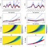 |
Fig. 1 Flux ratios for the individual progressions of H2 lines for simulated noisy data with relative flux errors of 0.05. We show the progressions as indicated at the lower or upper right corner of each panel. The line quotient gives the wavelength of the two involved lines for each ratio. They are ordered by increasing wavelength difference between the two lines. In the four upper panels, the black dots show the theoretical flux ratios. The red dots show the flux ratios from the simulated line fluxes. The black lines show the ratios of the dereddened flux (together with the dereddened flux error ratios) forRV=3.1 and AV=0.0,0.5,1.0,1.5,3.0. The red and blue lines denote the same for RV=2.1 and 4.1 for AV=1.0 and 3.0, respectively. We note that some of the lines are almost identical, which again indicating the degeneracy of RV and AV. Three of the four lower panels show contour plots for an increasingly worse fitting of the RV and AV values. We show the 68%, 90%, and 95% confidence interval as a black, blue, and yellow line, respectively. The numbers in these lines state the C ~ χ2s for the respective confidence level and are also given in the color bar. The red dot marks the position of the minimum of the distribution, and the black asterisks mark the values chosen for the simulation. In the bottom right panel, we overplot the 160 best-fit Cs for every progression. The progression [1,7] is represented by cyan dots, progression [1,4] is represented by blue triangles, and progression [0,1] is represented by red asterisks. Our retrieved extinction values are marked as a black dot with error bars. |
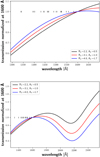 |
Fig. 2 Transmission calculated for AV and RV pairs as given in the legend and normalized at 1600 Å, which marks the longest wavelength of the lines we considered. The small vertical bars mark the position of the lines we used. Top: our considered wavelength range. Bottom: zoom out to show that lines at longer wavelength would probably allow us to break the degeneracy. |
3.2 Possible problems with self-absorption
The determination of AV from the UV H2 lines may be hampered by optical depth effects, that is, by self-absorption in the lines: when the levels are thermally populated, this leads to higher populations for the lower vibrational levels. Therefore, the lower vibrational levels have a higher probability of absorbing a fluoresced photon along the line of sight before the photon can escape from the protoplanetary disk. It might be re-emitted out of the line of sight, causing increasing flux loss for increasingly lower levels, which corresponds to lines at increasingly bluer wavelength. This higher opacity for bluer lines mimics the effect of extinction, as was first found by Wood et al. (2002). McJunkin et al. (2016) addressed this interplay between extinction and selfabsorption with two-step radiative transport calculations. In a first step, the lines blueward of 1450 Å are used to determine the self-absorption and a correction for it. In a second step, all lines are then used to determine AV. Since AV is not applied to the first step, however, the effect of self-absorption might be overestimated. Even in the case of TW Hya, where no complication by reddening is expected, the results are ambiguous because McJunkin et al. (2016) found a significant opacity in all lines below 1450 Å, while Herczeg et al. (2006) found that progressions [1,4] and [0,1] only have a significant optical depth for lines below 1300 and 1350 Å, respectively. Moreover, Ardila et al. (2002) found that the H2 levels for different stars with ν″ ≥4 are optically thin. The latter finding would allow us to use all of our lines in the analysis, but following Herczeg et al. (2004) would suggest that we omit the bluest line of the [0,1] progression. The study by McJunkin et al. (2016) would imply that the two bluest lines of progressions [0,1] and [0,2] are affected by non-negligible line opacity, and that to a smaller extent, even progressions [1,7] and [1.4] may be affected because their bluest lines are located around 1450 Å.
To gain further insight without applying full radiative transfer calculations, we estimated the optical depth τlu in the lines of the four progressions by using Eqs. (1)–(12) from McJunkin et al. (2016) with the Voigt profile of all lines set to unity. We took the lines in the four progressions into account as well as their pumping transitions near Lyα, and we neglected all other H2 lines. Considering only the pumping lines (since their level population numbers are expected to be much higher than the population numbers of the other transitions) and under the assumption of τ = 1, we calculated the total column density log(Ntot) ~ 15.5 for an assumed excitation temperature Texc = 2000 K. McJunkin et al. (2016) found average values of log(Ntot) = 19.0 (with DR Tau as an outlier with log(Ntot) = 15.1) and Texc = 1500 K (with TW Hya as an outlier with Texc = 2500 K). This discrepancy of our high-excitation temperatures leading to rather low column densities can be explained by our omission of all pumping lines blueward of the Lyα line center, which should have even higher population numbers. Moreover, a realistic Voigt profile would lead to higher column densities, as would a τlu for the pumping lines higher than one. We therefore consider our Ntot value as a lower limit, although it increases (slightly) with temperature.
In a second step, we then computed τlu in the individual (fluorescent) lines using Ntot. We list the τlu values we estimated under these assumptions in Table 2. As a result of our simplifications, these numbers should be treated with care, but we are positive that we recover the trend, confirming that progression [0,2] is much more affected than progressions [1,7] and [1,4]. Since the bluest line of progression [0,2] is most affected, this progression indeed cannot be used because other lines cannot be used due to blends.
With these general considerations in mind, we wished to rely only on the measured line flux and refrained from performing full radiative transport calculations to estimate the line opacity effects. Our motivation was to infer the lines that may be influenced by self-absorption from our derived AV and RV values of the different progressions for the individual stars.
4 Results
From our simulations, we expected to be able to recover the essentially zero extinction of TW Hya and the other low AV stars. For the other stars, measuring RV independently from AV may not lead to significant results given the noise level of the data and the degeneracy between RV and AV. Still, assuming RV=3.1, we expected to be able to measure AV. We list our results for all stars in Table 3 and show our results graphically for a representative selection of stars, like in the following example of TW Hya in the figures published on Zenodo.
We present our results for TW Hya graphically in Fig. 3 as an instructive example. Similar to Fig. 1, we show in the upper four panels the measured and the theoretical ratios for each progression. We realized that all theoretical ratios involving the line at 1442 Å from progression [1,7] are below the measured ratios, and therefore, the measured fluxes must be erroneous, because they cannot be reached by any dereddening, as shown by the colored curves. Since the line is near the beginning of an echelle order of the STIS spectrograph, we omitted it from the analysis The same is true for the line at 1547 Å from progression [1,4], which is severely blended with C IV. Fig. 3 shows for progression [1,7] that two additional theoretical values are below the measured values. Both ratios involve the line (1–7)R(6) at 1500.45 Å, which shows a satisfying fit. Since the deviation is only small and within the 3σ error for the measured values, we still used the ratios.
For TW Hya, we find an overall AV=0.3±0.1 mag and RV=1.65±0.15. We therefore conclude that our analysis for TW Hya favors a low but nonzero AV in combination with a very steep RV.
For the other six stars with low AV literature values, we find best-fit values of AV = 0.0 mag (for a wide variety of formal RV values for the individual stars). AV at RV=3.1 agrees with 0.0 mag within one standard deviation for all these stars (except for TW Hya). We show the obtained fits in figures published on Zenodo (see Table 3).
The stars with nonzero AV fall in three categories depending on the number of progressions that can be used to infer AV (which we therefore list in Table 3): in the first category, all three progressions led to about the same result. In the second category, the [0,1] progression led to deviating results and was omitted because the deviation of this progression might be self-absorption. In the third category, all three progressions led to differing results. In this last category, we found six stars for which the fit did not lead to an overlapping result region, and we were unable to assign an AV and RV value to these stars. Nevertheless, we computed a mean AV value for the case of an assumed RV = 3.1. We did this also for all other stars to allow for a better comparison to the literature values.
Best-fit results for AV and RV.
5 Discussion
We show our mean AV values derived for RV=3.1 in a comparison to literature AV values obtained for the same RV in Fig. 4. The Pearson correlation coefficients are r = 0.70 and p = 3.5 × 10⁻⁶, which indicates a correlation. The correlation is even better when we omit TW Hya, which would leave us with r = 0.80 and p = 2.7 × 10⁻⁸. TW Hya is special in the sense that it strongly deviates between the best AV values assigned by the box fit of 0.3 ± 0.1, with RV=1.65 and the best mean AV=1.2 for RV=3.1. McJunkin et al. (2016) also reported it as one of two stars for which the optical depth affected the lines up to 1450 Å. This may also slightly influence our progressions [1,7] and [1,4], which would (incorrectly) lead to higher AV values. Herczeg et al. (2004) found an AV=1.3 mag for TW Hya by ignoring the optical depth effects. This strongly suggests that for TW Hya, apart from the degeneracy, our results seem to be influenced by self-absorption, which we could not identify for this star because progressions [1,7] and [1.4] may also be influenced.
For the other six stars with literature AV = 0 mag, we also find very low to zero AV values with the box search method, as for a mean AV at RV=3.1. For three stars, low RV values are preferred by the box search, which may be caused at least partly by the degeneracy of AV and RV, since we do not find RV < 2.0 for the stars with nonzero AV. Moreover, for five of these seven stars, progression [0,1] leads to significantly higher AV values. This suggests a contamination by the optical depth for these stars. McJunkin et al. (2016) included TW Hya, DM Tau, RECX- 11, and RECX-15 in their study and found strong optical depth effects for wavelengths up to 1450 Å for these stars. After a correction for optical depth, they inferred high RV values for these stars, and in particular, for TW Hya also a high AV = 2.0. We agree with McJunkin et al. (2016) for the high optical depth in DM Tau, RECX-11, and RECX-15, but were unable to find indications of an optical depth in the H2 lines for TW Hya (which may be affected most, which means that our procedure failed; see above). Furthermore, our box search method prefers low RV values, which is in contrast to what McJunkin et al. (2016) found, except for RECX-11, where we find a comparably high RV value.
For the stars with nonzero AV, we have six stars in common with McJunkin et al. (2016): AA Tau, DE Tau, DR Tau, HN Tau, LkCa 15, and UX Tau. For the four stars AA Tau, DE Tau, HN Tau, and LkCa 15, the [0,1] progression leads to higher AV values, but for AA Tau and HN Tau, all three progressions differ. This is also the case for DR Tau, but progression [0,1] does not lead to the highest AV values and therefore does not indicate any optical depth effects. For UX Tau, we find the AV values of progression [0,1] to be only slightly higher than those of the other two progressions. McJunkin et al. (2016) found that optical depth played a role for five of these stars only for a wavelength below ~ 1300 Å, while for UX Tau, the affected region extended up to 1350 Å. The former would not affect any of our lines, while the latter would affect the bluest line of progression [0,1]. It is also curious that the stars for which McJunkin et al. (2016) found the weakest influence of the optical depth are the stars for which in our analysis all three progressions differ. This discrepancy for the individual stars remains unexplained. Spectra with a higher resolution would help us to distinguish between problems introduced by the method or physical properties, such as H2 emission, which partly originates in different places, for example, in the disk wind.
Figure 4 shows that our AV values, for which we used three progressions, are all equal to or higher than the literature values, which can be caused by the unattended self-absorption in the [0,1] progression. Of the stars for which we used only two progressions, slightly more than half exhibit a lower AV than the literature value, and we therefore argue that they are usually not influenced by optical depth.
An interesting question is whether H2 extinction measurements lead to different results than extinction measurements obtained from the optical for some physical reason. This may be expected because we measure extinction toward the origin of the H2 emission in the disk, while the measurements obtained from optical data determine extinction toward the star. We therefore show in Fig. 4 the extinction values color-coded with disk inclination, where low values indicate face-on disks. We find a tendency for face-on disks to show higher H2 measured than in the literature extinction. This might indicate that the light generated in the hot disk gas must pass the outer rims of the disk, while the light from the star is unaffected by this additional extinction. However, we only have three stars (TW Hya, DK Tau A, both with a face-on disk, and DE Tau) for which our extinction value is 3σ higher than the literature value.
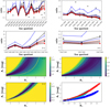 |
Fig. 3 Determination of AV for TW Hya. We show the progressions as indicated in the lower or upper right corner of each panel. The top four panels show the measured and dereddened flux ratios (red dots) and the theoretical flux ratios (black dots if the ratio is used for the analysis, gray otherwise). Each black line corresponds to the curve defined by the dereddend measured ratios according to RV=3.1 and AV=0.0,0.5,1.0,1.5,3.0. The red and blue lines denote the same for RV=2.1 and 4.1 for AV=1.0 and 3.0, respectively (the vertical bars are the dereddened errors of the ratios). Three of the four lower panels show the corresponding contour plots of the best-fit models in the RV–AV plane. We show the 68%, 90%, and 95% confidence interval as a black, blue, and yellow line, respectively. The numbers in these lines state the C ~ χ2s for the respective confidence level and are also given in the color bar. The red dot marks the position of the minimum of the distribution. In the bottom right panel, we overplot the 180 best-fit Cs for every progression. Progression [1,7] is represented by cyan dots, progression [1,4] is represented by blue triangles, and progression [0,1] is represented by red stars. The black dot with error bars marks the central position and extent of the search box, and it marks the overall best RV – AV combination. |
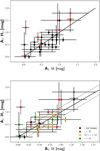 |
Fig. 4 Comparison of our AV values for fixed RV = 3.1 to the literature values. Top: when all three progressions could be used to infer the mean AV, the stars are represented by red dots, and when two progressions could be used, they are shown with black dots (progression [0,1] omitted). The black line indicates identity. The four stars with literature values of AV=0.0 mag are offset by 0.02 mag for clarity of their error bars. Bottom: same as above, but color-coded with the disk inclination. The dashed gray lines indicate errors of 0.2 mag. |
6 Conclusions
We derived AV and RV values for 34 CTTSs using measurements of fluoresced H2 line fluxes. Using simulated data, we showed that it is possible to recover AV and RV values for the typical S/N of the UV data using stars with literature values of AV ranging from 0 to 1.6 mag.
Our method used the theoretical line ratios separately for the individual progressions and combined the results from the individual progressions afterward. It allowed us to identify lines that are incompatible with the expected ratio pattern and therefore may be prone to systematic flux measurement errors, for example, by a blend with another line. We computed C values (similar to χ2 values) for the individual progressions on an AV and RV grid and applied a box search to identify the best-fitting models. This also partly allowed us to break the degeneracy between AV and RV and to obtain results for the AV and RV parameters.
In this way, we found low AV and RV values for the stars with AV=0.0 mag in the literature. For TW Hya and fixing RV=3.1, we found a significant AV=1.2±0.3 mag, without any indications of contamination by self-absorption. Although this may indicate that for TW Hya all our progressions are affected by optical depth effects, it may also indicate additional UV extinction in the vicinity of the star because for most other stars with face-on disks our AV values are also higher than the literature values.
For stars with nonzero AV literature values, we found lower as well as higher RV values than the canonical RV=3.1. For a mean AV obtained from two or three progressions at RV=3.1, we found reasonable agreement with literature values.
For the progressions we used, we found that progression [0,2] cannot be used due to a combination of unusable lines and because it is affected by self-absorption. For many stars, the same is true for progression [0,1], which was excluded from the AV determination when it exhibited systematically steeper RV –AV distributions than the other progressions. Progressions [1,4] and [1,7] seem to be usable for all stars (except perhaps for TW Hya).
In summary, the exact AV values that we derived may be affected by some systematic uncertainties such as optical depth effects. However, the values that result from the simple reconstruction are quite close to the literature values and only allow some but not much additional UV extinction in the vicinity of the warm disk, where the H2 fluorescent lines are created.
We therefore argue that the H2-derived AV values, and the literature AV for that matter, are good estimates of the extinction toward the inner warm disk. The general agreement between the literature and our H2-based AV values suggests that no (significant) additional extinction sources exist between the star and the disk.
We found no indication for additional UV extinction either, for instance, by steep extinction laws. This is particularly relevant when modeling the UV spectra of accreting stars because our values provide an estimate of the UV-AV that cannot be exceeded. Specifically in the context of models that describe the stellar UV spectrum as a combination of accretion columns, it is possible that some of these accretion fluxes can be immediately absorbed in the vicinity of the star, but our results indicate no additional UV-extinction. Therefore, the H2-based or standard AV values should also be used to redden the calculated UV emission from the accretion columns for comparison with observations.
In the future, better (higher S/N) UV H2 line fluxes together with simultaneously treated extinction and optical depth will eventually allow one to derive the extinction toward the inner disk.
Data availability
The figures published via Zenodo can be downloaded under https://zenodo.org/records/14034355
Acknowledgements
The authors acknowledge funding through Deutsche Forschungsgemeinschaft DFG program IDs EI 409/20-1 and SCHN 1382/4-1 in the framework of the YTTHACA project (Young stars at Tübingen, Tautenburg, Hamburg & ESO – A Coordinated Analysis). Funded by the European Union under the European Union’s Horizon Europe Research & Innovation Programme 101039452 (WANDA). Views and opinions expressed are, however, those of the author(s) only and do not necessarily reflect those of the European Union or the European Research Council. Neither the European Union nor the granting authority can be held responsible for them. Based on observations obtained with the NASA/ESA Hubble Space Telescope, retrieved from the Mikulski Archive for Space Telescopes (MAST) at the Space Telescope Science Institute (STScI). STScI is operated by the Association of Universities for Research in Astronomy, Inc. under NASA contract NAS 5-26555. This work benefited from discussions with the ODYSSEUS team (HST AR-16129, Espaillat et al. 2022, https://sites.bu.edu/odysseus/) and especially with G. J. Herczeg and K. Grankin. This work made use of PyAstronomy (Czesla et al. 2019), which can be downloaded at https://github.com/sczesla/PyAstronomy.
Appendix A Total flux in a single progression (Method II)
Here we discuss an alternative method that is conceptually even simpler than the method introduced above but lacks certain diagnostics, which makes it inferior in the end. This alternative method is based on the fact that photon flux in an individual line,  , is given by the total flux F[i, k] in progression [i,k] by
![Mathematical equation: $F_{ij}^* = F[i,k] \cdot {B_{ij}},$](/articles/aa/full_html/2024/12/aa52086-24/aa52086-24-eq8.png) (A.1)
(A.1)
where Bij is the accompanying branching ratio, defined as Bij = Aij/ Σ A[i,k] with the spontaneous emission Einstein coefficient Aij. Since we measure the reddened energy flux  this leads to
![Mathematical equation: $F_{ij}^\prime = \tau \left( {\lambda ;{A_V},{R_V}} \right) \cdot F[i,k] \cdot {{hc} \over {{\lambda _{ij}}}} \cdot {B_{ij}},$](/articles/aa/full_html/2024/12/aa52086-24/aa52086-24-eq10.png) (A.2)
(A.2)
where τ(λ; AV, RV) is the transmission for wavelength λ due to reddening and  converts photon flux to energy flux. For a more detailed discussion we refer to Appendix A.1.
For any progression [i,k] and n measured line fluxes in that progression, this leads to a set of n equations with the three free parameters: F[i, k], RV and AV; the latter two determine τ(λ, AV, RV). Therefore, n ≥ 3 lines would be already sufficient to provide an extinction estimate, and more lines can be used to optimize the result using, e. g. the χ2 method. In fact, only three or four H2 lines provide reliable line fluxes in some progressions.
The extension from using only one progression to using more progressions is straight forward, since each additional progression introduces only one additional unknown to the set of equations as AV and RV stay the same. Therefore a large number of progressions with each having several measured line fluxes is desirable.
We chose progressions [1,7], [1,4], and [0,1] for this method, since test calculations for our stars show that progression [0,2] only enlarged χ2 without altering the results notably. Moreover, we use an AV and RV grid for the optimization and fit only the F[a,b] values for each AV and RV-pair; we then record the χ2- value for each AV and RV-pair and determine the best extinction values together with its confidence range from these χ2-values.
To test this approach, we simulated data like for Method I and show the results in Fig. A.1 for random realizations of the ‘observed’ flux vector. Figure A.1 shows that small relative errors usually allow us to recover AV, even RV for small or negligible measurement errors. For the data at hand, a relative error of 0.05 best describes the measurements and allows us to recover AV values from 0.0 mag to 0.5 mag, while larger errors introduce subsequently larger uncertainties.
A.1 Detailed derivation of Method II
The line emissivity (units: erg cm−3 s−1) of a transition from an upper level ν = v′, J′ to an lower level l = ν″, J″ is given by
 (A.3)
(A.3)
with Aul being the Einstein coefficient, nu the number density of the energy level Eu, and Eul being the energy difference between the two states. The energy difference for each transition is associated with the release of a photon at wavelength λul via
 (A.4)
(A.4)
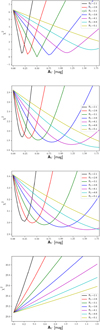 |
Fig. A.1 Retrieval of AV by χ2 for different RV as marked in the legend for simulated data. Input data is RV=3.1 and AV=0.5 mag except for the lower right panel, where AV=0.0 mag Top: Relative error of 0.01, but no statistical noise in the data. Upper middle: Relative error of 0.05, also noise in the data. Lower middle: Relative error of 0.10, also noise in the data. Bottom: Relative error of 0.05, also noise in the data. |
At this point we introduce the branching ratio for a progression:
![Mathematical equation: ${B_{ul}} = {{{A_{ul}}} \over {\sum\nolimits_{\left[ {v',J'} \right]} {{A_{ul}}} }},$](/articles/aa/full_html/2024/12/aa52086-24/aa52086-24-eq14.png) (A.5)
(A.5)
where the sum goes over all transitions in the progression [ν′, J′]. Bul can be interpreted as probability of the transition u → l, since
![Mathematical equation: $\sum\limits_{\left[ {{v^\prime },{J^\prime }} \right]} {{B_{ul}}} = 1.$](/articles/aa/full_html/2024/12/aa52086-24/aa52086-24-eq15.png) (A.6)
(A.6)
For N considered transitions, i.e. number of lines in a progression, we can calculate the following expression using Eqs. A.3 and A.5:
![Mathematical equation: ${{{j_{ul}}} \over {{B_{ul}}{E_{ul}}}} = {1 \over {4\pi }}{n_u}\sum\limits_{\left[ {{v^\prime },{J^\prime }} \right]} {{A_{ul}}} .$](/articles/aa/full_html/2024/12/aa52086-24/aa52086-24-eq16.png) (A.7)
(A.7)
Equation A.7 gives the same constant for every transition, i.e. it is independent of the considered transition u → l We can add all these expressions for the N transitions to arrive at
![Mathematical equation: ${1 \over N}\sum\limits_{\left[ {{v^\prime },{J^\prime }} \right]} {{{{j_{ul}}} \over {{B_{ul}}{E_{ul}}}}} = {1 \over {4\pi }}{n_u}\sum\limits_{\left[ {{v^\prime },{J^\prime }} \right]} {{A_{ul}}} .$](/articles/aa/full_html/2024/12/aa52086-24/aa52086-24-eq17.png) (A.8)
(A.8)
By summing up all emissivities divided by their individual branching ratios and individual photon energy we get a constant that depends only on the sum of all relevant Einstein coefficients.
The Method I described here utilises the N equations (Eq. A.7) in the following way: The extinction law with parameters AV and RV is a wavelength dependent function, here introduced as τ(λ; AV, RV), which reduces effectively the intrinsic line emissivities  to the observed line emissivities
  via
via
 (A.9)
(A.9)
Introducing the extinction into Eq. A.7 leads to a new set of N equations, which are now
![Mathematical equation: ${1 \over {4\pi }}{n_u}\sum\limits_{\left[ {{v^\prime },{J^\prime }} \right]} {{A_{ul}}} = {{j_{ul}^{{\rm{int}}}} \over {{B_{ul}}{E_{ul}}}} = {{{\tau ^{ - 1}}\left( {{\lambda _{ul}};{A_V},{R_V}} \right) \cdot j_{ul}^{{\rm{obs}}}} \over {{B_{ul}}{E_{ul}}}}.$](/articles/aa/full_html/2024/12/aa52086-24/aa52086-24-eq21.png) (A.10)
(A.10)
Incorporating Eq. A.4 into Eq. A.10 leads to
![Mathematical equation: ${{{\tau ^{ - 1}}\left( {{\lambda _{ul}};{A_V},{R_V}} \right) \cdot j_{ul}^{{\rm{obs}}} \cdot {\lambda _{ul}}} \over {{B_{ul}}}} = 1/4\pi hc \cdot {n_u}\sum\limits_{\left[ {{v^\prime },{J^\prime }} \right]} {{A_{ul}}} = {\rm{const}}{\rm{.}}$](/articles/aa/full_html/2024/12/aa52086-24/aa52086-24-eq22.png) (A.11)
(A.11)
From observations we can measure the N line fluxes and therefore line emissivities (see the next section) and get a set of N equations with three parameters AV, RV, and the constant.
In the following we give an example with 4 measured lines, where j51, j52, j53, j54 are the measured line emissivities, A51, A52, A53, A54 are the Einstein coefficients, and λ51, λ52, λ53, λ54 are the photon wavelengths. The set of N = 4 equations are


If one observes for an individual star a second progression, the constant C changes, but AV and RV stay the same, so that just one additional variable is added and another N′ equations, depending on the number N′ of observed lines in the second progression.
In Method II we use line fluxes and not emissivities. Here we show, how one gets from the line emissivities jul (units: erg cm−3 s−1) to the integrated line fluxes Ful (units: erg cm−2 s−1 ): The emitting gas is confined to a volume Vemit located at the distance D to the observer. The total energy per unit time in an emission line u → l radiated from the emitting gas is then
 (A.12)
This is the line luminosity (units: erg s−1). The integrated line flux is then given by
 (A.13)
If all emission lines emerge from the same volume at the same distance we have
 (A.14)
Therefore, we can substitute the line emissivities with the line fluxes,
 (A.15)
holds, though with a different constant.
A.2 AV derived with Method II
We show our results exemplarily in Fig. A.2 for the stars TW Hya, DK Tau A, SY Cha, and MY Lup, which worked best using Method I in the sense, that all three progressions could be used. Since for no star a distinct χ2 minimum can be identified we stick to a fixed RV=3.1. We estimate the 1σ variance in AV by using χ2 + 1. For TW Hya we do not get AV=0 mag, instead for RV=3.1 we measure an AV = 1.3 ± 0.5 mag, which should be clearly too high for this star, though also Method I leads to a similar value, if RV=3.1 is chosen. Our overall lowest χ2 measurement corresponds to AV = 0.5 ± 0.2 mag and RV=2.1, which indicates a very steep extinction law but is in agreement with our Method I. The low RV value may be caused by the H2 lines at wavelength lower than about 1450 Å not being optically thin any more.
For SY Cha we also obtain AV = 1.3 ± 0.75 mag for a fixed RV=3.1, which is in agreement with Method I. Fixing RV to the preferred value of Method I, to 2.1, would lead to identical values of AV=0.5 mag for Method I and Method II. For DK Tau A we derive AV = 1.4±0.9 mag, which is in agreement with Method I. For MY Lup we derive AV = 1.1 ± 0.7 mag, which is lower than the value obtained with Method I. Nevertheless, Method I yields consistent results, if we there also fix RV=3.1.
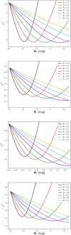 |
Fig. A.2 Estimation of AV by χ2 for different RV as marked in the legend. Top: For TW Hya. Upper middle: For SY Cha. Lower middle: For DK Tau. Bottom: For MY Lup. |
Unfortunately, Method II leads generally to large error bars that prevent us from identifying unique values for AV for the individual stars. However, the error ranges for all stars except TW Hya overlap if one allows for the low RV value.
A.3 Comparison of the two methods
Method I has several advantages over Method II. First, while we treat all progressions together in Method II, for Method I we treat each progression separately and combine these then into one result for the AV of each star. Though this merging of the results comes with difficulties, it allows progressions with differing contributions to be identified. Second, if theoretical ratios lower than the observed ratios are found, the pattern in the quotients affected often allows to identify the line, which may contribute an erroneous flux. Since only some of these lines show also unacceptable Gaussian fits, this allows for some additional ’hand-picking’ of the used lines. We think that the better usage of the information content of the measurements together with the better control of error introducing drawbacks of Method I is allowing us to break the degeneracy of AV and RV (at least partly) by comparing the different progressions.
References
- Abgrall, H., Roueff, E., Launay, F., Roncin, J. Y., & Subtil, J. L. 1993, A&AS, 101, 273 [NASA ADS] [Google Scholar]
- Alcalá, J. M., Manara, C. F., Natta, A., et al. 2017, A&A, 600, A20 [NASA ADS] [CrossRef] [EDP Sciences] [Google Scholar]
- Ardila, D. R., Basri, G., Walter, F. M., Valenti, J. A., & Johns-Krull, C. M. 2002, ApJ, 566, 1100 [NASA ADS] [CrossRef] [Google Scholar]
- Calvet, N., Briceño, C., Hernández, J., et al. 2005, AJ, 129, 935 [CrossRef] [Google Scholar]
- Cardelli, J. A., Clayton, G. C., & Mathis, J. S. 1989, ApJ, 345, 245 [Google Scholar]
- Carvalho, A. S., & Hillenbrand, L. A. 2022, ApJ, 940, 156 [NASA ADS] [CrossRef] [Google Scholar]
- Czesla, S., Schröter, S., Schneider, C. P., et al. 2019, PyA: Python astronomyrelated packages [Google Scholar]
- Draine, B. T. 2003, ARA&A, 41, 241 [NASA ADS] [CrossRef] [Google Scholar]
- Espaillat, C. C., Herczeg, G. J., Thanathibodee, T., et al. 2022, AJ, 163, 114 [NASA ADS] [CrossRef] [Google Scholar]
- Fitzpatrick, E. L. 1999, PASP, 111, 63 [Google Scholar]
- France, K., Arulanantham, N., Maloney, E., et al. 2023, AJ, 166, 67 [CrossRef] [Google Scholar]
- Gangi, M., Nisini, B., Manara, C. F., et al. 2023, A&A, 675, A153 [NASA ADS] [CrossRef] [EDP Sciences] [Google Scholar]
- Grankin, K. N. 2017, in Astronomical Society of the Pacific Conference Series, 511, Non-Stable Universe: Energetic Resources, Activity Phenomena, and Evolutionary Processes, eds. A. M. Mickaelian, H. A. Harutyunian, & E. H. Nikoghosyan, 37 [Google Scholar]
- Green, J. C., Froning, C. S., Osterman, S., et al. 2012, ApJ, 744, 60 [NASA ADS] [CrossRef] [Google Scholar]
- Hartigan, P., & Morse, J. 2007, ApJ, 660, 426 [NASA ADS] [CrossRef] [Google Scholar]
- Herczeg, G. J., & Hillenbrand, L. A. 2014, ApJ, 786, 97 [Google Scholar]
- Herczeg, G. J., Linsky, J. L., Valenti, J. A., Johns-Krull, C. M., & Wood, B. E. 2002, ApJ, 572, 310 [NASA ADS] [CrossRef] [Google Scholar]
- Herczeg, G. J., Wood, B. E., Linsky, J. L., Valenti, J. A., & Johns-Krull, C. M. 2004, ApJ, 607, 369 [NASA ADS] [CrossRef] [Google Scholar]
- Herczeg, G. J., Linsky, J. L., Walter, F. M., Gahm, G. F., & Johns-Krull, C. M. 2006, ApJS, 165, 256 [NASA ADS] [CrossRef] [Google Scholar]
- Hoadley, K., France, K., Alexander, R. D., McJunkin, M., & Schneider, P. C. 2015, ApJ, 812, 41 [NASA ADS] [CrossRef] [Google Scholar]
- Ingleby, L., Calvet, N., Herczeg, G., et al. 2013, ApJ, 767, 112 [Google Scholar]
- Jordan, C., Brueckner, G. E., Bartoe, J. D. F., Sandlin, G. D., & van Hoosier, M. E. 1977, Nature, 270, 326 [NASA ADS] [CrossRef] [Google Scholar]
- Kenyon, S. J., & Hartmann, L. 1995, ApJS, 101, 117 [Google Scholar]
- Luhman, K. L., Mamajek, E. E., Shukla, S. J., & Loutrel, N. P. 2017, AJ, 153, 46 [Google Scholar]
- Manara, C. F., Testi, L., Herczeg, G. J., et al. 2017, A&A, 604, A127 [NASA ADS] [CrossRef] [EDP Sciences] [Google Scholar]
- Mathis, J. S. 1990, ARA&A, 28, 37 [NASA ADS] [CrossRef] [Google Scholar]
- McJunkin, M., France, K., Schneider, P. C., et al. 2014, ApJ, 780, 150 [NASA ADS] [CrossRef] [Google Scholar]
- McJunkin, M., France, K., Schindhelm, R., et al. 2016, ApJ, 828, 69 [NASA ADS] [CrossRef] [Google Scholar]
- Miller, J. S. 1968, ApJ, 154, L57 [NASA ADS] [CrossRef] [Google Scholar]
- Predehl, P., & Schmitt, J. H. M. M. 1995, A&A, 293, 889 [NASA ADS] [Google Scholar]
- Rieke, G. H., & Lebofsky, M. J. 1985, ApJ, 288, 618 [Google Scholar]
- Roman-Duval, J., Proffitt, C. R., Taylor, J. M., et al. 2020, RNAAS, 4, 205 [NASA ADS] [Google Scholar]
- Rucinski, S. M., & Krautter, J. 1983, A&A, 121, 217 [NASA ADS] [Google Scholar]
- Rugel, M., Fedele, D., & Herczeg, G. 2018, A&A, 609, A70 [NASA ADS] [CrossRef] [EDP Sciences] [Google Scholar]
- Schindhelm, R., France, K., Herczeg, G. J., et al. 2012, ApJ, 756, L23 [NASA ADS] [CrossRef] [Google Scholar]
- Schneider, P. C., France, K., Günther, H. M., et al. 2015, A&A, 584, A51 [NASA ADS] [CrossRef] [EDP Sciences] [Google Scholar]
- Schneider, P. C., Manara, C. F., Facchini, S., et al. 2018, A&A, 614, A108 [NASA ADS] [CrossRef] [EDP Sciences] [Google Scholar]
- Schultz, G. V., & Wiemer, W. 1975, A&A, 43, 133 [NASA ADS] [Google Scholar]
- Shull, J. M. 1978, ApJ, 224, 841 [NASA ADS] [CrossRef] [Google Scholar]
- Sternberg, A. 1988, ApJ, 332, 400 [NASA ADS] [CrossRef] [Google Scholar]
- Welty, D. E., & Fowler, J. R. 1992, ApJ, 393, 193 [NASA ADS] [CrossRef] [Google Scholar]
- Wood, B. E., Karovska, M., & Raymond, J. C. 2002, ApJ, 575, 1057 [NASA ADS] [CrossRef] [Google Scholar]
All Tables
All Figures
|
Fig. 1 Flux ratios for the individual progressions of H2 lines for simulated noisy data with relative flux errors of 0.05. We show the progressions as indicated at the lower or upper right corner of each panel. The line quotient gives the wavelength of the two involved lines for each ratio. They are ordered by increasing wavelength difference between the two lines. In the four upper panels, the black dots show the theoretical flux ratios. The red dots show the flux ratios from the simulated line fluxes. The black lines show the ratios of the dereddened flux (together with the dereddened flux error ratios) forRV=3.1 and AV=0.0,0.5,1.0,1.5,3.0. The red and blue lines denote the same for RV=2.1 and 4.1 for AV=1.0 and 3.0, respectively. We note that some of the lines are almost identical, which again indicating the degeneracy of RV and AV. Three of the four lower panels show contour plots for an increasingly worse fitting of the RV and AV values. We show the 68%, 90%, and 95% confidence interval as a black, blue, and yellow line, respectively. The numbers in these lines state the C ~ χ2s for the respective confidence level and are also given in the color bar. The red dot marks the position of the minimum of the distribution, and the black asterisks mark the values chosen for the simulation. In the bottom right panel, we overplot the 160 best-fit Cs for every progression. The progression [1,7] is represented by cyan dots, progression [1,4] is represented by blue triangles, and progression [0,1] is represented by red asterisks. Our retrieved extinction values are marked as a black dot with error bars. |
| In the text | |
|
Fig. 2 Transmission calculated for AV and RV pairs as given in the legend and normalized at 1600 Å, which marks the longest wavelength of the lines we considered. The small vertical bars mark the position of the lines we used. Top: our considered wavelength range. Bottom: zoom out to show that lines at longer wavelength would probably allow us to break the degeneracy. |
| In the text | |
|
Fig. 3 Determination of AV for TW Hya. We show the progressions as indicated in the lower or upper right corner of each panel. The top four panels show the measured and dereddened flux ratios (red dots) and the theoretical flux ratios (black dots if the ratio is used for the analysis, gray otherwise). Each black line corresponds to the curve defined by the dereddend measured ratios according to RV=3.1 and AV=0.0,0.5,1.0,1.5,3.0. The red and blue lines denote the same for RV=2.1 and 4.1 for AV=1.0 and 3.0, respectively (the vertical bars are the dereddened errors of the ratios). Three of the four lower panels show the corresponding contour plots of the best-fit models in the RV–AV plane. We show the 68%, 90%, and 95% confidence interval as a black, blue, and yellow line, respectively. The numbers in these lines state the C ~ χ2s for the respective confidence level and are also given in the color bar. The red dot marks the position of the minimum of the distribution. In the bottom right panel, we overplot the 180 best-fit Cs for every progression. Progression [1,7] is represented by cyan dots, progression [1,4] is represented by blue triangles, and progression [0,1] is represented by red stars. The black dot with error bars marks the central position and extent of the search box, and it marks the overall best RV – AV combination. |
| In the text | |
|
Fig. 4 Comparison of our AV values for fixed RV = 3.1 to the literature values. Top: when all three progressions could be used to infer the mean AV, the stars are represented by red dots, and when two progressions could be used, they are shown with black dots (progression [0,1] omitted). The black line indicates identity. The four stars with literature values of AV=0.0 mag are offset by 0.02 mag for clarity of their error bars. Bottom: same as above, but color-coded with the disk inclination. The dashed gray lines indicate errors of 0.2 mag. |
| In the text | |
|
Fig. A.1 Retrieval of AV by χ2 for different RV as marked in the legend for simulated data. Input data is RV=3.1 and AV=0.5 mag except for the lower right panel, where AV=0.0 mag Top: Relative error of 0.01, but no statistical noise in the data. Upper middle: Relative error of 0.05, also noise in the data. Lower middle: Relative error of 0.10, also noise in the data. Bottom: Relative error of 0.05, also noise in the data. |
| In the text | |
|
Fig. A.2 Estimation of AV by χ2 for different RV as marked in the legend. Top: For TW Hya. Upper middle: For SY Cha. Lower middle: For DK Tau. Bottom: For MY Lup. |
| In the text | |
Current usage metrics show cumulative count of Article Views (full-text article views including HTML views, PDF and ePub downloads, according to the available data) and Abstracts Views on Vision4Press platform.
Data correspond to usage on the plateform after 2015. The current usage metrics is available 48-96 hours after online publication and is updated daily on week days.
Initial download of the metrics may take a while.