| Issue |
A&A
Volume 692, December 2024
|
|
|---|---|---|
| Article Number | A250 | |
| Number of page(s) | 13 | |
| Section | Extragalactic astronomy | |
| DOI | https://doi.org/10.1051/0004-6361/202451906 | |
| Published online | 19 December 2024 | |
Towards a complete census of luminous Compton-thick active galactic nuclei in the Local Universe
1
Institute for Astronomy Astrophysics Space Applications and Remote Sensing (IAASARS), National Observatory of Athens, Ioannou Metaxa & Vasileos Pavlou, Penteli 15236, Greece
2
School of Physics and Astronomy, University of Southampton, Highfield, Southampton SO17 1BJ, UK
3
Cahill Center for Astrophysics, California Institute of Technology, 1216 East California Boulevard, Pasadena, CA 91125, USA
4
Physics Department, University of Durham, South Road, Durham DH1 3LE, UK
⋆ Corresponding author; ig@noa.gr
Received:
16
August
2024
Accepted:
7
October
2024
X-ray surveys provide the most efficient means for the detection of active galactic nuclei (AGNs). However, they do face difficulties in detecting the most heavily obscured Compton-thick AGNs. The BAT detector on board the Gehrels/Swift mission, operating in the very hard 14–195 keV band, has provided the largest samples of Compton-thick AGN in the Local Universe. However, even these flux-limited samples may miss the most obscured sources among the Compton-thick AGN population. A robust way to find these local sources is to systematically study volume-limited AGN samples detected in the IR or the optical part of the spectrum. Here, we utilise a local sample (< 100 Mpc) of mid-IR-selected AGNs, unbiased against obscuration, to determine the fraction of Compton-thick sources in the Local Universe. When available, we acquired X-ray spectral information for the sources in our sample from previously published studies. In addition, to maximise the X-ray spectral information for the sources in our sample, we analysed eleven unexplored XMM-Newton and NuSTAR observations, for the first time. In this way, we identified four new Compton-thick sources. Our results reveal an increased fraction of Compton-thick AGNs among the sources that have not been detected by BAT of 44%. Overall, we have estimated a 25–30% share of Compton-thick sources in the Local Universe among mid-IR-selected AGNs. We find no evidence for any evolution of the AGN Compton-thick fraction with luminosity.
Key words: galaxies: active / quasars: supermassive black holes
© The Authors 2024
 Open Access article, published by EDP Sciences, under the terms of the Creative Commons Attribution License (https://creativecommons.org/licenses/by/4.0), which permits unrestricted use, distribution, and reproduction in any medium, provided the original work is properly cited.
This article is published in open access under the Subscribe to Open model. Subscribe to A&A to support open access publication.
1. Introduction
X-ray emission is ubiquitous in active galactic nuclei (AGNs) and it is believed to originate from a corona above the accretion disk (e.g. Haardt & Maraschi 1991). According to this scenario, the UV photons produced in the accretion disk are scattered by the hot coronal electrons having temperatures of about 60 keV (Akylas & Georgantopoulos 2021) and producing copious amounts of X-ray emission. The X-ray radiation that permeates the sky, namely, the X-ray background (Giacconi et al. 1962) in the energy range of 0.1–300 keV, is produced by the superposition of AGNs. The Chandra X-ray mission owing to its superb spatial resolution resolved about 90% of the X-ray background in the relatively soft 0.5–8 keV band (Mushotzky et al. 2000). Indeed, optical spectroscopic observations confirm that the vast majority of these sources are associated with AGNs, with redshifts peaking at z ≈ 0.7 (e.g. Luo et al. 2017).
Observations with the Gehrels/Swift/BAT (Ajello et al. 2008), RXTE (Revnivtsev et al. 2003), BeppoSAX (Frontera et al. 2007), and Integral (Churazov et al. 2007) missions show that the peak energy density of the X-ray background lies at harder energies around 30 keV. The X-ray background synthesis models attempt to reproduce the spectrum of the X-ray background by modeling the AGN luminosity function together with their spectral properties (Comastri et al. 1995; Gilli et al. 2007; Treister et al. 2009; Akylas et al. 2012; Ueda et al. 2014; Ananna et al. 2019). All X-ray background models find that in order to reproduce the 30 keV energy hump, we need a considerable fraction of heavily obscured Compton-thick AGNs. However, the exact fraction depends on the amount of reflection in the vicinity of the emitted radiation that is the accretion disk and the surrounding torus (Gandhi et al. 2007; Vasudevan et al. 2013). In Compton-thick sources, the line-of-sight to the nucleus is obscured by huge amounts of gas with column densities exceeding NH ≈ 1024 cm−2. The obscuring screen is believed to be a dusty structure with toroidal geometry. Recent observations suggest that this obscuring screen, the torus, is composed of optically thick clouds Nenkova et al. (2002, 2008), Tristram et al. (2007). In Compton-thick AGNs, the obscuration is because of Compton-scattering rather than photoelectric absorption. The X-ray photons below 10 keV are almost totally absorbed and, hence, X-ray observations at higher energies are necessary to securely classify a source as a Compton-thick AGN. The exact fraction of Compton-thick sources among the total AGN population differs significantly among the various X-ray background models. Akylas et al. (2012) estimated a rather modest fraction, namely, about 20% or lower (see also Treister et al. 2009; Vasudevan et al. 2013). On the other end, the models of Ananna et al. (2019) have shown that Compton-thick AGNs could constitute half of the AGN population.
The launch of the Gehrels/Swift mission Gehrels et al. (2004) constituted a leap forward in the study of Compton-thick AGNs owing to its hard energy range. The Burst Alert Telescope, BAT, onboard Gehrels/Swift continuously scans the whole sky in the 14–195 keV band. Therefore, BAT provided an unprecedented census of the hard X-ray sky and, in particular, of Compton-thick AGNs. Ricci et al. (2015), Akylas et al. (2016) analysed AGN X-ray spectra in the BAT 70-month survey (Baumgartner et al. 2013), finding a few tens of candidate Compton-thick AGNs. In addition, Marchesi et al. (2018), Zhao et al. (2021), and Torres-Albà et al. (2021) searched for Compton-thick AGNs on the Palermo 100-month BAT catalogue. Using the BAT sample, Akylas et al. (2016) and, most recently, Ananna et al. (2022) derived for the first time the Compton-thick AGN luminosity function in the Local Universe. More recently, Georgantopoulos et al. (2024) revisit these luminosity functions using the most up-to-date column density estimates derived by NuSTAR. According to the works cited above, the fraction of Compton-thick AGNs should not exceed 25% of the total AGN population (see also Burlon et al. 2011; Ricci et al. 2015; Georgantopoulos & Akylas 2019; Torres-Albà et al. 2021).
Nevertheless, the Compton-thick AGNs detected by BAT may be the tip of the iceberg. This is because even the BAT band (14–195 keV) may miss a significant fraction of heavily obscured AGNs. Burlon et al. (2011) found that even mildly Compton-thick AGNs, with a column density of a few times 1024 cm−2, are attenuated by 50% in the hard 15–55 keV band. The most heavily obscured, reflection-dominated Compton-thick AGNs with column densities of NH ≈ 1025 cm−2 such as NGC 1068 have the bulk of their 15–55 keV flux attenuated. In order to find the most heavily obscured AGNs, we have to resort to volume-limited optically selected or IR-selected AGNs. Along these lines, Akylas & Georgantopoulos (2009) observed with XMM-Newton all (38) Seyfert-2 galaxies in the Palomar spectroscopic sample of galaxies (Ho et al. 1997). They find that the fraction of Compton-thick sources among Seyfert-2 galaxies is about 20%. Recently, Asmus et al. (2020) compiled the most complete so far galaxy sample in the Local Universe (< 100 Mpc). They selected AGNs applying the selection criteria based on the WISE W1-W2 colour (Assef et al. 2018). This sample comprises about 150 sources and has been routinely observed by most X-ray missions. For these sources, we compiled previously published results and we analysed, for the first time, the X-ray spectra of eleven sources. Our goal is to provide the most definitive yet estimate of the fraction of Compton-thick sources among the WISE-selected AGNs in the Local Universe.
Our paper is organised as follows. In Sect. 2, we describe in detail the sample of Asmus et al. (2020) and the selection criteria applied. In Sect. 3, we detail the new X-ray observations obtained by NuSTAR, XMM-Newton, and Chandra. The spectral fit results are presented in Sect. 4. The discussion and the summary are presented in Sects. 5 and 6, respectively.
2. The sample
In this work, we utilise data from the Local AGN survey (LASr) sample, (Asmus et al. 2020), which provides the most complete census of mid-IR selected AGNs among all galaxies within a volume of 100 Mpc. The sample contains 49 k galaxies and has a completeness of 90% at log M⋆/M⊙ = 9.4. Then, the applied WISE identification criteria serve as a robust tracer of AGN emission. Briefly, the sources selected satisfy the following criteria: (a) the W1 (3.4 μm) and W2 (4.6 μm) AGN selection criterion from (Assef et al. 2018). This criterion is based on the hot emission coming from the AGN heated obscuring torus, becoming prominent at short mid-IR wavelengths(< 50 μm); (b) the theoretical colour criterion based on the WISE W2 and W3 (12 μm) presented in Satyapal et al. (2018), to separate AGNs from luminous starbursts; and (c) L(12μm) > 1042.3 erg s−1. According to Asmus et al. (2020), the above criteria ensure a reliability of over 90% for finding an AGN.
Consequently, the authors cited above derived two AGN datasets. The first is the ‘known AGN’ sample containing WISE-selected AGNs, already known to host an active nucleus in the literature. The second is the ‘new AGN’ sample, which contains the WISE selected AGNs that have no prior AGN classifications in the literature.
In this study, we primarily focus on the ‘known AGN’ sample. This is because the ‘new AGN’ sample has practically no X-ray information available. On the other hand, as anticipated, the ‘known AGN’ sample contains a large fraction of sources (approximately 75%) detected within XMM-Newton, NuSTAR, or BAT observations. The remaining sources (about 25%) are not present in the above archives and lack usable X-ray data. Among the remaining sources, fewer than 30% fall within the footprint of Gehrels/Swift/XRT observations and even fewer cases allow for the extraction of a poor-quality X-ray spectrum.
In Fig. 1, we compare the redshift distribution of the sources within these two sub-samples. Notably, the majority of the sources lacking X-ray data are concentrated in the highest redshift bin, namely, between 0.02 and 0.022. At lower redshift values the fraction of the sources without X-ray data is very small. Based on this plot and with the goal of improving the X-ray completeness of our sample, we applied a cut at the redshift of z = 0.02 (∼87 Mpc).
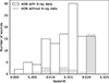 |
Fig. 1. Redshift distribution of the sources in the ‘known AGN’ sample. The solid line histogram represents the distribution of sources with available X-ray data and the gray shaded histogram the distribution of the sources without X-ray data. |
After applying all the selection criteria to the optically selected ‘known AGN sample’, we identified 113 AGNs. Among these, the largest number (72 sources) have also been detected in the 70-month Swift/BAT all-sky survey (Baumgartner et al. 2013). Their X-ray spectral properties have been systematically studied in detail in Ricci et al. (2017) primarily using XMM-Newton and Gehrels/Swift/BAT spectra. Additionally, several individual studies re-analysed specific cases, particularly those considered as Compton-thick candidates, also utilising NuSTAR observations.
Among the 41 sources that have not been detected by BAT, 14 have already been analysed using archival NuSTAR and/or XMM-Newton observations and their results have been presented in the literature. Additionally, a search within the NuSTAR and XMM-Newton archives yields good quality X-ray data for eleven additional sources which have not been reported in the literature. For the remaining sources, namely, those lacking NuSTAR XMM-Newton or BAT observations, we queried the Gehrels/Swift X-ray Telescope (XRT) Science Data Centre repository (Evans et al. 2009) to obtain the spectral fits (when possible). The cross-correlation with the XRT 2SXPS catalogue (Evans et al. 2020) reveals five sources with available spectral information. Thus, only eleven sources (i.e. less than 10%) of our sample remains without X-ray spectral information. After the above selections, our working sample with the available X-ray observation is composed of 102 sources (see Table 2). For the sake of completeness, we note that there are 32 sources in the ‘new AGN’ sample following the same mid-IR selection criteria, up to a redshift of z = 0.02.
The full list of our sources is available online (see Sect. 6) and in Table 1, we present a small part of this list. The X-ray spectral information is obtained from either from the literature or from our own spectral analysis. A detailed discussion of the newly analyzed sources is presented in Sects. 3 and 4.
Log of our sample (extract). The full catalogue is available at the CDS.
‘Known AGN’ sample.
3. New X-ray observations
In Table A.1, we present the X-ray log of the eleven sources with available archival XMM-Newton or NuSTAR X-ray data, which are presented for the first time in this work. In particular, five sources have both NuSTAR and XMM-Newton data and one source presents only NuSTAR and Chandra data, while five sources have only XMM-Newton observations available.
In the table, there is an additional entry, namely, the case of IC4995. Recently, Osorio-Clavijo et al. (2022) reported IC4995 as a Compton-thick AGN using the same NuSTAR data set presented here. However, their analysis employed a rather simple model. Given the Compton-thick nature of this source, we chose to re-analyze the same NuSTAR data in conjunction with XMM-Newton observations to derive more accurate estimations for its luminosity and column density.
In the case of the five sources in our sample with Gehrels/Swift/XRT data (marked with an s in Table 1), we have not performed the X-ray data reduction or analysis. The X-ray spectral data have been retrieved from the Gehrels/Swift/XRT Science Data Centre repository (Evans et al. 2020).
3.1. XMM-Newton data reduction
We restrict our analysis on XMM-Newton EPIC-pn data as they provide the highest source count rate. The observation data files (ODF) and the Pipeline Processing System (PPS) calibrated event lists of each observation are retrieved from the XMM-Newton Science Archive (XSA). These observations were then further processed using the XMM-Newton Science Analysis Software (SAS v21.0.0)1.
All the event files have been re-screened to remove background flares. To do so, we created a single event (PATTERN = 0), high-energy (10–12 keV) light curve for each observation. We visually inspected all these light curves and determined the threshold count rate (roughly varying between 0.1 and 0.5 count/s) below which the light curve is low and steady. Then we created the good time interval (GTI) file for each observation using TABGTIGEN task.
In our analysis, only single and double events (i.e. PATTERN < = 4 for the EPIC PN) have been used and, in addition, the flag = 0 selection expression has been applied to reject events that are close to CCD gaps or bad pixels. We defined a circular region of 15 arcsec in radius for the source area and a 50 arcsec nearby source-free region for the background estimation. Then the source and background files were produced using EVSELECT task and the corresponding auxiliary files were generated using RMFGEN and ARFGEN tasks. All the spectra have been grouped to give a minimum of 15 counts per bin.
3.2. NuSTAR data reduction
The NuSTAR observations are processed using the data analysis software NUSTARD AS v2.1.2 and CALDB v.202310172. We downloaded the calibrated event list files from the NuSTAR archive. An inspection of these cleaned event files showed no further affection by flaring events.
Then, we extracted the source and background event files for each of the two NuSTAR focal plane modules (FPMA & FPMB) using the NUPRODUCTS script. We adopted a radius of 60 arcsec for the source spectral extraction, for both FPMA and FPMB. The background spectra were extracted from a four times larger (120 arcsec radius) source-free region of the image at an off-axis angle close to the source position.
3.3. Chandra data reduction
During the single Chandra observation presented here, the ACIS was operating in the ACIS-S mode. Our data reduction for the Chandra observation was performed using CIAO v.4.15 and the CALDB version 4.10.7. We used the level 2, fully calibrated events, provided by the Chandra X-Ray Center standard pipeline process. We extracted the spectral and the ancillary files using the SPECEXTRACT script in CIAO. The source spectrum was extracted from a circular area of 5 arcsec radius, while the background spectrum was extracted from a nearby, source-free circle of 20 arcsec radius. The spectrum was grouped using the GRPPHA task in FTOOLS to a minimum number of 15 counts per bin.
4. Spectral analysis
In this work, we present the X-ray spectral analysis for twelve sources. Eleven sources are presented for the first time here, whereas IC4995, already presented in Osorio-Clavijo et al. (2022), has been re-analyzed with a model more suitable to its Compton-thick nature. The spectral fitting was carried out using XSPEC v12.13.1 (Arnaud 1996). We simultaneously fit all the available spectra for each source.
4.1. Single power-law model
Initially, we utilised a simple model consisting of an absorbed power-law model (PO) to describe the AGN continuum X-ray emission. We also tried to add a Gaussian component (GA) to account for the FeKα emission line and/or a thermal model (APEC) and/or a second soft power-law to accommodate the possible presence of starforming or scattered soft X-ray emission. These additional components are added to the data when they provide an improvement to the fit at the 90 per cent confidence level.
The full XSPEC notation of our model is PHABSGAL*(APEC+PO+zPHABS*PO+zGA). The Galactic value of the equivalent hydrogen column for the photoelectric absorption model (PHABS) is being fixed to the value obtained from Dickey & Lockman (1990); while the intrinsic column density of the source is free to vary. The source redshift is also fixed to the spectroscopic values presented in Table 2. The abundances have been fixed to the default abundance table values in XSPEC and the width of the Gaussian line is also freeze to 0.01 keV.
Only three sources are consistent with this model. The reduced χ2 value (which is close to 1) suggests a good fit. These lack a strong absorption or high FeKα equivalent width. The spectral fitting results for these three sources are listed in Table A.2. In particular, we list the value of the plasma temperature for the thermal model, photon index of the power-law along with the estimated amount of obscuration, equivalent width of the FeKα line, and the normalisation parameters of the continuum. A goodness of fit estimator is also presented using the χ2 statistic over the degrees of freedom (χ2/d.o.f.). All the errors correspond to the 90% confidence level. Moreover, Table A.5, lists the estimated flux and luminosity values for each component used in the fitting. In particular, we provide the observed flux of the soft components and the continuum flux in the 0.5–2, 2–10 and 10–80 keV bands. Estimates in the ultra hard 10–80 keV band are presented only when NuSTAR data are available. We also present the intrinsic luminosity measurements of the same components by zeroing the value of the intrinsic column density in the best fit model.
In Fig. 2, we plot the unfolded spectrum, the best fit model and the residuals in E2f(E) units. This representation visualises the spectral fitting results and distinguishes between the different spectral components. We note that in the E2f(E) plot, a photon index of Γ = 2 is represented by a horizontal line. The thermal emission is shown as an increase above the hard X-ray continuum in the lower energies, while absorption effects appear as a constant decline of the spectrum towards lower energy part of the spectrum.
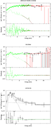 |
Fig. 2. X-ray spectra, best fit model and residuals for the sources fitted with the simple model. |
4.2. RXTORUS model
For the majority of the sources, the spectral fitting results using the above simple model do not provide an acceptable fit. This is primarily due to the estimated column density being sufficiently high, close to or exceeding the Compton-thick limit. Consequently, Thompson scattering effects must also be considered through appropriate modeling. Moreover, in these cases, the reflected emission may be a dominant process in shaping of the hard X-ray spectrum. If not properly addressed, this can result in unrealistic X-ray spectral indexes and inaccurate fitting outcomes.
To address these complexities, we opted to utilise the RXTORUS model introduced by Paltani & Ricci (2017). This model self-consistently addresses: (a) the transmitted continuum, containing only photons that did not interact with the surrounding material; (b) the scattered continuum, containing all photons that underwent one or more Compton scatterings, but no photo-ionisation or fluorescence; and (c) all photons that underwent at least one photo-ionisation and subsequent fluorescence re-emission, in addition to any number of Compton scatterings.
The free model parameters are: (a) the power-law photon index; (b) the column density along the line of sight; (c) the equatorial column density of the torus, (d) the inclination angle, defined as the angle between the normal to the plane of the torus and the observer; (e) the opening angle of the torus defined as the ratio of the inner to the outer radius of the torus; and (f) the normalisation factor. In our case, we used the RXTORUS model grid calculated with a pre-fixed high energy cut-off value of 200 keV and the abundances are fixed to the default abundance table values used in the XSPEC (Anders & Grevesse 1989). In our set-up, we assume a simple torus geometry and, therefore, the equatorial column density and the line-of-sight obscuration are tied using Eq. (1) in Paltani & Ricci (2017). Also, the normalisation parameters of the reprocessed emission are tied to the normalisation of the continuum.
As in the case of the simple modeling presenting above, we checked for the presence of a thermal model (APEC) and/or a second soft power-law to account for any starforming or scattered soft X-ray emission. These additional components are added to the data when they provide and improvement to the fit at at least a 90 per cent confidence level. The XSPEC notation of this model is PHABSGAL∗(PO+APEC+RXTORUS), where the RXTORUS notation corresponds to the XSPEC command atable(RXTORUS reprocessed component)+etable(RXTORUS continuum component)*CUTOFFPL.
In specific cases, depending on the quality of the data and model complexity, we chose to freeze certain model parameters to aid in fitting and prevent convergence issues. Thus, the photon index is sometimes fixed at the value of Γ = 2, the viewing angle is set to 90 degrees (edge-on) and the ratio of the inner to the outer radius is fixed at 0.5, corresponding to a half torus opening angle of 60 degrees.
The spectral fitting results using the above spectral model are presented in Table A.3. In detail, we list the thermal model plasma temperature, the photon index of the scattered emission (Γsoft), the photon index of the continuum power-law along, the obscuration along the line of sight, and the corresponding equatorial column density. The values for the torus opening angle and the viewing angle are also listed in the same table. An estimate of the goodness-of-fit is also provided using χ2/d.o.f. ratio. Model components that are not statistically significant are omitted from the table. Fixed parameter values and upper limit estimations are clearly indicated in the table. All errors correspond to the 90% confidence interval. Notably, all the sources are reasonably well fit using the RXTORUS model. Moreover, in Table A.6, we provide a comprehensive summary of the estimated flux and luminosity for each of the model components used in the fitting as discussed previously in the case of the simple spectral modeling. Additionally, in Fig. 3 we plot the unfolded spectrum, the best fit model and the residuals in E2f(E) units.
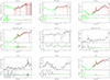 |
Fig. 3. X-ray spectra, best fit model, and residuals for the sources fitted with the RXTORUS model. |
Our spectral analysis suggests that all sources present column densities exceeding 1023 cm−2. In particular, there are four Compton-thick sources, reported for the first time in the literature: ESO420-013, UGC01214, 2MASXJ04405494-0822221, and IC4769. In three cases, we can only provide a lower limit on NH estimation utilising both NuSTAR and XMM-Newton data. Only in the case of IC4769, the NH constraint is tighter, which is, however, achieved by fitting the only available XMM-Newton data with a fixed photon index. A common characteristic is the very prominent FeKα emission line, present in all the individual observations. This further supports the presence of high amounts of obscuring material along their line of sight.
In all sources strong soft excess emission is being observed, originating from optically thin collisionally ionised hot plasma (APEC model component). Additionally, most sources require an additional scattered emission component (soft power-law component) to adequately fit the soft X-ray data. When the data do not provide a reasonable constraint, the photon indices of both the soft and hard power-law components are tied and fixed to a value of Γ = 2. However, in certain cases, decoupling the photon index of the scattered emission from that of the intrinsic emission as suggested by, in Silver et al. (2022) and Yamada et al. (2021) leads to a significantly improved spectral fits.
4.3. UXCLUMPY model
For the five Compton-thick sources presented in Table A.3, we repeated the spectral fitting analysis using the UXCLUMPY model (Buchner et al. 2019). This model was constructed to reproduce the column density distribution of the AGN population and cloud eclipse events in terms of their angular sizes and frequency. The model assumes a clumpy structure for the obscuring material and applies a second Compton thick reflecting layer close to the corona. Our motivation is to verify the Compton-thick nature of these sources using a substantially different fitting model. An equally important task is to explore whether the UXCLUMPY model, allowing for a much higher values for the column density than any other model (up to 1026 cm−2), could provide tighter constrains for the column density of these sources. To this end, we used a similar setup as described previously; however all the geometrical parameters have been kept fixed. The viewing angle, measured from the vertical symmetry axis toward the equator has been fixed to 90 degrees. The σtorus parameter (TORsigma in XSPEC table model) that describes the dispersion of the cloud population has been fixed to 30 degrees and the covering factor of the Compton thick inner reflecting layer (CTKcover parameter) has been fixed to 0.4. The results are presented in Table A.4. The new spectral fitting results verify the Compton-thick nature of these sources. However, we were unable to further constrain the NH values, which still appear as lower limits.
5. Discussion
We organise our discussion as follows. In Sect. 5.1, we present the NH distribution among the ‘known AGN’ sample. In Sect. 5.2, we discuss about the prospects of finding a large number of Compton-thick AGNs among the ‘new AGN’ sample that has no BAT detections. It is likely that a number of Compton-thick sources may lie among the AGNs that have not been selected by the WISE criteria (further discussed in Sect. 5.3). In Sect. 5.4, we discuss the Compton-thick AGNs that may be lurking among the fainter AGN sub-sample with luminosities logL(12 μm) [erg s−1]< 42.3. In Sect. 5.5 we discuss the possible dependence of the fraction of either obscured or Compton-thick AGNs on luminosity. Finally, in Sect. 5.6, we argue on the existence of extremely obscured AGNs with NH > 1025 cm−2.
5.1. Compton-thick sources in the ‘known AGN’ sample
While X-ray surveys offer the most unobscured view towards the nucleus, when these sources are obscured by material close to or above the Compton thick limit (where the Compton scattering processes dominate over photo-ionisation), the X-ray sources suffer from significant attenuation hindering their detection. This results in a bias in the sense that higher column density sources are under-represented in flux-limited surveys, even those in the BAT ultra hard X-ray band. Hence, the recovery of the true fraction of Compton-thick AGNs, even in the Local Universe, remains problematic. Our analysis enables us to study the distribution of obscuration in the Local Universe in a nearly unbiased way, as it is based on a complete volume-limited galaxy sample.
In Fig. 4, we present the NH distribution, along the line of sight, for the sources in our sample. The upper panel compares the NH distribution of the 70-month BAT AGNs existing in our sample (grey-shaded histogram), with the NH distribution of the sources missed by the hard X-ray survey (red-dashed line). The bottom panel shows the total NH distribution of our sources. Notably, the vast majority of the sources missed by the BAT survey (14 out of 30) are associated with Compton-thick sources corresponding to a fraction of 45%. This clearly suggests that below the BAT flux limit there is a population of Compton-thick AGNs lurking, which have evaded detection. For all the 102 sources in our sample, the fraction of Compton-thick AGNs is 25/102 or 25 ± 5%.
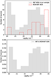 |
Fig. 4. The NH distribution for the sources in our sample. (a) Upper panel: Comparison of the NH distribution for the sources in our sample detected in Gehrels/Swift/BAT 70 months all sky survey (grey-shaded histogram) with those missed (red-dashed line). (b) Lower panel: NH distribution for the total population. |
In Fig. 5, we compare the intrinsic 2–10 keV luminosity distribution of the BAT detected and non-detected sample. It is noteworthy that a non-negligible number of sources within the non-BAT sample extends to lower luminosities, Lx < 1041.5 erg s−1, forming a tail in the distribution. The vast majority of these sources are not Compton-thick. Two of these have been analysed for the first time here, namely, NGC 3094 an UGC04145 showing no evidence for significant obscuration. Another source, (NGC 2623) is moderately obscured (Yamada et al. 2021), while only NGC 660 shows evidence for significant obscuration Annuar et al. (2020). This suggests that a number of sources remain undetected by BAT because they have a low intrinsic luminosity rather than being associated with Compton-thick sources. Similar conclusions are drawn by Yamada et al. (2021, 2023) in a sample of nearby ultra-luminous infrared galaxies.
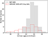 |
Fig. 5. Comparison of the 2–10 keV luminosity distribution for the sources detected in Gehrels/Swift/BAT 70 month-long all-sky survey (grey-shaded histogram) with those missed (red-dashed line). |
An unknown factor that may affect our estimations is the number of sources lacking X-ray information. For these sources the column density and the X-ray luminosity remain unknown and, as a result, they have not been included in the analysis. In Fig. 6, we compare the redshift and the 12 micron luminosity, L12 μm, derived from Asmus et al. (2020), with the rest of our sample. The redshift distribution of the X-ray undetected sources shows no difference compared to the rest of the sample. However, the L12 μm distribution clearly occupies the low luminosity part of the distribution, L12 μm < 1043 erg s−1. This suggests that a number of sources have not been detected because they have low luminosities rather than they are associated with Compton-thick nuclei. In the extreme case, where we assume that all eleven sources without X-ray information are associated with Compton-thick AGNs, the fraction would rise to 32 ± 5%.
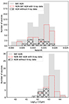 |
Fig. 6. The redshift and luminosity distributions for the sources in our sample. (a) Upper panel: Comparison of the redshift distribution for the sources in our sample according to their origin. Sources found in BAT surveys are shown with gray histogram, sources with X-ray data missed by BAT survey are displayed with red-dashed line and sources without X-ray data are shown with the hatched histogram. (b) Lower panel: Similar as above for the L12 μm luminosity obtained from Asmus et al. (2020). |
5.2. WISE-selected AGNs with no X-ray data available
So far, we have covered the properties of the ‘known AGN’ sample, containing (as explained at Sect. 2) WISE-selected AGNs, already known to host an active nucleus in the literature. As we mentioned, Asmus et al. (2020) defined an additional AGN sample or the ‘new AGN’ sample, containing WISE-selected AGNs, using the same criteria, but without any prior AGN classification in the literature. This sample comprises of 32 ‘new’ AGNs. At first glance, we would expect that the fraction of Compton-thick AGN is high and, hence, the ‘new’ AGNs remain undetected by BAT. Indeed, the fraction of Compton-thick AGNs in the ‘known AGN’ sample that were undetected by BAT was particularly high, namely, of the order of 45%. The comparison of the L12 μm-z distribution of the BAT AGNs and the ‘new AGN’ sample (Fig. 7) sheds more light on the reasons why the latter sample may remain undetected in BAT. The distribution of the ‘new AGN’ sample is clearly skewed towards lower luminosities and higher redshift. This suggests that a number of the ‘new’ AGNs may remain undetected by BAT because of their low luminosity, provided that there is a strong correlation between the L12 μm and the X-ray luminosity, as found in Asmus et al. (2015) and Stern (2015). According to the above diagram, the most strong candidates for being Compton-thick sources are a handful of sources that mingle with the ‘known AGN’ sample in the same luminosity-redshift area.
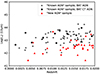 |
Fig. 7. L12 μm vs. redshift distribution of the BAT AGNs against the ‘new’ AGN sample. |
5.3. Compton-thick AGNs missed by the WISE criteria
A number of well-known, BAT-detected, Compton-thick AGNs are not present in our sample. This is because of the applied AGN selection criteria, based on the WISE colours presented in Sect. 2. For example, a number of low-luminosity AGNs or those where the emission from the host galaxy dominates over the AGN may be missed by the W1-W2 criterion (e.g. Pouliasis et al. 2020). Then, a question arises as to whether our sample selection criteria affect the fraction of detected Compton-thick sources.
To investigate this issue, we examined the sample of Compton-thick AGNs compiled by the Clemson group (e.g. Marchesi et al. 2018; Zhao et al. 2021; Torres-Albà et al. 2021). These Compton-thick AGNs were originally selected from the BAT AGN catalogue. Then, the column density was accurately determined by means of NuSTAR observations. There are 17 bona fide Compton-thick AGNs in the Clemson sample3 within z < 0.02. Only 8 out of these 17 Compton-thick sources follow our selection criteria (presented in Sect. 2), while 9 Compton-thick sources in the Clemson sample do not; therefore, they have been missed from this study. However, in a similar manner, in Gehrels/Swift/BAT 70 month, all-sky survey, there are approximately 145 sources identified as AGNs within z < 0.02, according to Baumgartner et al. (2013). From this sample, half of the sources (72) satisfy the same WISE selection criteria while the other half (73) have been missed. This exercise clearly demonstrates that our selection criteria equally affect all the BAT population and not preferentially the highly obscured sources. Therefore, the measured fraction of Compton thick sources remains unaffected, at least for the fluxes probed by the Gehrels/Swift/BAT 70 month, all-sky survey.
5.4. Compton-thick AGNs at faint luminosities
Up to this point, we have discussed the presence of Compton-thick sources among luminous AGNs with luminosities logL(12 μm) [erg s−1]> 42.3, regardless of their blue or red W1-W2 colours. However, Asmus et al. (2020) pointed out that 70% of known Seyferts have luminosities below this threshold. This means that an appreciable number of low-luminosity Compton-thick AGNs may remain undetected. We used the relation of hard X-ray luminosities versus the nuclear MIR luminosities (e.g. Gandhi et al. 2009; Asmus et al. 2011) to convert our 12 μm luminosity threshold to a 2–10 keV X-ray luminosity threshold. We find that the corresponding 2–10 keV X-ray luminosity is approximately log LX [erg s−1]> 42.2. It has been suggested that the fraction of obscured AGNs increases with decreasing luminosity or decreasing Eddington ratio (e.g. Akylas et al. 2006; Ezhikode et al. 2017; Ueda et al. 2014). However, at very low luminosities, this trend may be reversed. According to theoretical models no torus is formed at very low bolometric luminosities, LBOL < 1042 erg s−1 (Elitzur & Shlosman 2006). In any case, such a population of low luminosity Compton-thick AGNs may indeed exist without violating the hard X-ray and mid-IR background constraints (Comastri et al. 2015; Nardini & Risaliti 2011). We note here that Boorman et al. (2024) presented simulations, suggesting that the new High-Energy X-ray Probe-class mission concept (HEX-P) will be able to measure intrinsic luminosities and line-of-sight column densities, while also distinguishing between obscuration geometries of this low-luminosity population.
5.5. Dependence of obscuration on luminosity
Next, we investigated whether there is a dependence of the Compton-thick fraction on intrinsic luminosity. If, for example, the fraction of Compton-thick AGNs increases with decreasing luminosity, this could imply that the X-ray undetected sources in our sample harbour more heavily obscured sources. Previous results on this subject remain controversial. In particular Brightman et al. (2015) found possible evidence of a strong decrease of the covering factor of the torus, while Buchner et al. (2015) found instead that the fraction of Compton-thick AGNs is compatible with being constant with the X-ray luminosity. Also, Ricci et al. (2015) analyzed the data from the Gehrels/Swift/BAT all-sky survey and provided the corrected for selection bias, intrinsic column density distribution of Compton-thick AGNs in the Local Universe in two different luminosity ranges. Their average estimated fraction of Compton-thick sources is 27 ± 4%. They also present tentative evidence for a small decrease in the fraction of obscured Compton-thick AGNs with increasing luminosity. In Fig. 8, we present the fraction of the Compton-thick sources in our sample as a function of the 2–10 keV and the 12 micron luminosity. The errors in the estimated Compton-thick fraction correspond to the 1σ confidence level and the uncertainty in the luminosity denotes the range of each luminosity bin. Clearly, the plots show no evidence for any dependence of the Compton-thick fraction with luminosity. Our results indicate a very similar fraction of Compton-thick sources at all luminosity bins, fully consistent with the average value of 25 ± 5%. However the limited statistics do not allow us to rule out changes at the level of the quoted errors.
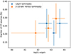 |
Fig. 8. Fraction of the Compton-thick sources (NH > 1024 cm−2) in our sample as a function of the intrinsic 2–10 keV luminosity (blue-squared points) and the 12 micron luminosity (orange-circled points). The error in the estimated fraction corresponds to the 68 per cent confidence level while the uncertainty in the luminosity axis denotes the range of each luminosity bin used. |
Next, we plot the fraction of the obscured sources (NH > 1022 cm−2) as a function of the intrinsic luminosity in Fig. 9. Previous studies (e.g. Ueda et al. 2003; Akylas et al. 2006; Buchner et al. 2015; Ricci et al. 2015) suggest a clear decline in the fraction of obscuration with decreasing X-ray luminosity. Our analysis does not reveal any such trend, which stands in contradiction to the studies above. However, this trend has been previously identified across a much broader luminosity range than the one explored here and, in fact, the highest luminosity bins (not covered here) play the most significant role with respect to this trend (e.g. Ueda et al. 2003).
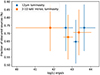 |
Fig. 9. Fraction of the obscured sources (NH > 1022 cm−2) as a function of the intrinsic 2–10 keV luminosity (blue-square points) and the 12 micron luminosity (orange-circle points). The error in the estimated fraction corresponds to the 68 per cent confidence level while the uncertainty in the luminosity axis denotes the range of each luminosity bin used. |
Alternatively, Sazonov et al. (2015), claim that this effect could be purely artificial due to a negative bias in finding obscured sources and a positive bias in finding unobscured AGNs, due to the reflected emission. According to these authors, the above biases lead to a decreasing observed fraction of obscured AGNs with increasing luminosity even if there is no intrinsic luminosity dependence. In this scenario, the current analysis correctly finds a constant fraction of obscured sources in all luminosities.
5.6. Extreme obscuration in the Local Universe
Our work thus far provides a robust and almost unbiased constraint on the Compton-thick fraction among the bright, WISE-selected AGNs in the Local Universe. One key element, which has not been addressed, is the distribution of the column density among the Compton-thick sources. Most X-ray background synthesis models assume either a flat fraction of Compton-thick AGNs over the entire range of log(NH) [cm−2]=24 − 26 (e.g. Ananna et al. 2019; Ueda et al. 2014; Gilli et al. 2007); alternatively, all Compton-thick AGNs are placed in the range of log(NH) [cm−2]=24 − 25 (e.g. Akylas et al. 2016). Our observational leverage on the distribution remains uncertain. The only two known Compton-thick AGNs, which may have column densities close to ∼NH = 1025 cm−2, are Circinus and NGC 1068. The dearth of such highly obscured sources in the BAT surveys is possibly because the extreme obscuration prohibits their detection even at distances as low as 100 Mpc (e.g. Burlon et al. 2011). The limited NH range of the current Compton-thick spectral models, which typically have a ceiling in the maximum allowed NH value of 1025 cm−2, further complicates the secure identification of the most heavily obscured of the Compton-thick sources.
Our sample which does not suffer from any flux-limit bias offers the opportunity to further address this issue. We arbitrarily assume that all the Compton-thick sources with lower limit column density estimations, NH > 1024 cm−2, occupy the log(NH) [cm−2]=25 − 26 bin. All the other Compton-thick sources (those with a secure measurement in their NH) are then placed in the log(NH) [cm−2]=24 − 25 bin. According to Table 1, there are 25 Compton-thick sources in our sample and only in eight cases the NH estimation is a lower limit. Then, this crude approximation shows that the fraction of log(NH) [cm−2]=25 − 26 sources account roughly for at most 30% of the Compton-thick population at least in the ‘known AGN’ sample.
6. Summary
We analysed the X-ray properties of the sample compiled by Asmus et al. (2020) of local (z < 0.02) AGNs. Our basic goal in this work is to constrain the number density of Compton-thick sources. We primarily focus on the AGN sample selected on the basis of the WISE W1 and W2 colours, which is then divided in two subsamples. The ‘known AGN’ sample, already known to host an active nucleus in the literature, containing 113 sources; of these, the vast majority (102) have been observed by various X-ray missions (with 72 detected by BAT). The second is the ‘new AGN’ sample, containing 32 sources, which have no prior AGN classification in the literature. For the first sample, we compiled the X-ray observations available in the literature. We also analyse, for the first time, the NuSTAR, XMM-Newton and Chandra observations of eleven sources. As the sample examined here is not flux-limited, it offers us the best opportunity thus far to study the full Compton-thick AGN population. Our results can be summarised as follows.
-
Our spectral analysis employing both the RXTORUS and the UXCLUMPY models reveals four new Compton-thick sources with column densities in excess of 4 × 1024 cm−2.
-
The fraction of Compton-thick sources among the 102 sources with available X-ray data in the ‘known AGN’ sample is 25 ± 5%. Even in the extreme case where all the sources with no available X-ray data were associated with Compton-thick AGNs, the Compton-thick fraction would rise to 31 ± 5%.
-
The fraction of Compton-thick AGNs among the 30 sources that have not been detected by BAT is much higher (44%) compared to the fraction of the Compton-thick sources in the BAT detected sources, which is only 16%.
-
Regarding the ‘new AGN’ sample, we argue that most of these sources have not been detected by BAT because they have low luminosity, rather than high obscuration.
Our work provides a robust and almost unbiased constraint on the Compton-thick fraction among the bright, WISE-selected AGNs in the Local Universe. It is the lower-luminosity AGNs that still remain unexplored in the X-rays. The new, High-Energy X-ray mission ATHENA will be able to provide estimates on the intrinsic luminosities and line-of-sight column densities of this low-luminosity population shedding more light on the formation and evolution of the torus in AGNs.
Data availability
The full version of Table 1 is available at the CDS via anonymous ftp to cdsarc.cds.unistra.fr (130.79.128.5) or via https://cdsarc.cds.unistra.fr/viz-bin/cat/J/A+A/692/A250.
Acknowledgments
This research is based on observations obtained with XMM-Newton, an ESA science mission with instruments and contributions directly funded by ESA Member States and NASA. This research has made use of data from the NuSTAR mission, a project led by the California Institute of Technology, managed by the Jet Propulsion Laboratory, and funded by the National Aeronautics and Space Administration. Data analysis was performed using the NuSTAR Data Analysis Software (NuSTAR DAS), jointly developed by the ASI Science Data Center (SSDC, Italy) and the California Institute of Technology (USA). This research has made use of data obtained from the Chandra Data Archive and the Chandra Source Catalog, and software provided by the Chandra X-ray Center (CXC) in the application packages CIAO and Sherpa. This research has made use of data and software provided by the High Energy Astrophysics Science Archive Research Center (HEASARC), which is a service of the Astrophysics Science Division at NASA/GSFC. This research uses data supplied by the UK Swift Science Data Centre at the University of Leicester.
References
- Ajello, M., Greiner, J., Sato, G., et al. 2008, ApJ, 689, 666 [Google Scholar]
- Akylas, A., & Georgantopoulos, I. 2009, A&A, 500, 999 [NASA ADS] [CrossRef] [EDP Sciences] [Google Scholar]
- Akylas, A., & Georgantopoulos, I. 2021, A&A, 655, A60 [NASA ADS] [CrossRef] [EDP Sciences] [Google Scholar]
- Akylas, A., Georgantopoulos, I., Georgakakis, A., Kitsionas, S., & Hatziminaoglou, E. 2006, A&A, 459, 693 [NASA ADS] [CrossRef] [EDP Sciences] [Google Scholar]
- Akylas, A., Georgakakis, A., Georgantopoulos, I., Brightman, M., & Nandra, K. 2012, A&A, 546, A98 [NASA ADS] [CrossRef] [EDP Sciences] [Google Scholar]
- Akylas, A., Georgantopoulos, I., Ranalli, P., et al. 2016, A&A, 594, A73 [NASA ADS] [CrossRef] [EDP Sciences] [Google Scholar]
- Ananna, T. T., Treister, E., Urry, C. M., et al. 2019, ApJ, 871, 240 [Google Scholar]
- Ananna, T. T., Weigel, A. K., Trakhtenbrot, B., et al. 2022, ApJS, 261, 9 [NASA ADS] [CrossRef] [Google Scholar]
- Anders, E., & Grevesse, N. 1989, Geochim. Cosmochim. Acta, 53, 197 [Google Scholar]
- Annuar, A., Alexander, D. M., Gandhi, P., et al. 2020, MNRAS, 497, 229 [CrossRef] [Google Scholar]
- Arnaud, K. A. 1996, ASP Conf. Ser., 101, 17 [Google Scholar]
- Asmus, D., Gandhi, P., Smette, A., Hönig, S. F., & Duschl, W. J. 2011, A&A, 536, A36 [NASA ADS] [CrossRef] [EDP Sciences] [Google Scholar]
- Asmus, D., Gandhi, P., Hönig, S. F., Smette, A., & Duschl, W. J. 2015, MNRAS, 454, 766 [NASA ADS] [CrossRef] [Google Scholar]
- Asmus, D., Greenwell, C. L., Gandhi, P., et al. 2020, MNRAS, 494, 1784 [Google Scholar]
- Assef, R. J., Prieto, J. L., Stern, D., et al. 2018, ApJ, 866, 26 [NASA ADS] [CrossRef] [Google Scholar]
- Baumgartner, W. H., Tueller, J., Markwardt, C. B., et al. 2013, ApJS, 207, 19 [Google Scholar]
- Boorman, P. G., Torres-Albà, N., Annuar, A., et al. 2024, Front. Astron. Space Sci., 11, 1335459 [NASA ADS] [CrossRef] [Google Scholar]
- Brightman, M., Baloković, M., Stern, D., et al. 2015, ApJ, 805, 41 [NASA ADS] [CrossRef] [Google Scholar]
- Buchner, J., Georgakakis, A., Nandra, K., et al. 2015, ApJ, 802, 89 [Google Scholar]
- Buchner, J., Brightman, M., Nandra, K., Nikutta, R., & Bauer, F. E. 2019, A&A, 629, A16 [NASA ADS] [CrossRef] [EDP Sciences] [Google Scholar]
- Burlon, D., Ajello, M., Greiner, J., et al. 2011, ApJ, 728, 58 [Google Scholar]
- Churazov, E., Sunyaev, R., Revnivtsev, M., et al. 2007, A&A, 467, 529 [NASA ADS] [CrossRef] [EDP Sciences] [Google Scholar]
- Comastri, A., Setti, G., Zamorani, G., & Hasinger, G. 1995, A&A, 296, 1 [NASA ADS] [Google Scholar]
- Comastri, A., Gilli, R., Marconi, A., Risaliti, G., & Salvati, M. 2015, A&A, 574, L10 [NASA ADS] [CrossRef] [EDP Sciences] [Google Scholar]
- Dickey, J. M., & Lockman, F. J. 1990, ARA&A, 28, 215 [Google Scholar]
- Elitzur, M., & Shlosman, I. 2006, ApJ, 648, L101 [Google Scholar]
- Evans, P. A., Beardmore, A. P., Page, K. L., et al. 2009, MNRAS, 397, 1177 [Google Scholar]
- Evans, P. A., Page, K. L., Osborne, J. P., et al. 2020, ApJS, 247, 54 [Google Scholar]
- Ezhikode, S. H., Gandhi, P., Done, C., et al. 2017, MNRAS, 472, 3492 [NASA ADS] [CrossRef] [Google Scholar]
- Frontera, F., Orlandini, M., Landi, R., et al. 2007, ApJ, 666, 86 [NASA ADS] [CrossRef] [Google Scholar]
- Gandhi, P., Fabian, A. C., Suebsuwong, T., et al. 2007, MNRAS, 382, 1005 [NASA ADS] [CrossRef] [Google Scholar]
- Gandhi, P., Horst, H., Smette, A., et al. 2009, A&A, 502, 457 [NASA ADS] [CrossRef] [EDP Sciences] [Google Scholar]
- Gehrels, N., Chincarini, G., Giommi, P., et al. 2004, ApJ, 611, 1005 [Google Scholar]
- Georgantopoulos, I., & Akylas, A. 2019, A&A, 621, A28 [NASA ADS] [CrossRef] [EDP Sciences] [Google Scholar]
- Georgantopoulos, I., Pouliasis, E., Ruiz, A., & Akylas, A. 2024, A&A, submitted [arXiv:2412.05432], [Google Scholar]
- Giacconi, R., Gursky, H., Paolini, F. R., & Rossi, B. B. 1962, Phys. Rev. Lett., 9, 439 [NASA ADS] [CrossRef] [Google Scholar]
- Gilli, R., Comastri, A., & Hasinger, G. 2007, A&A, 463, 79 [NASA ADS] [CrossRef] [EDP Sciences] [Google Scholar]
- Haardt, F., & Maraschi, L. 1991, ApJ, 380, L51 [Google Scholar]
- Ho, L. C., Filippenko, A. V., & Sargent, W. L. W. 1997, ApJS, 112, 315 [NASA ADS] [CrossRef] [Google Scholar]
- Luo, B., Brandt, W. N., Xue, Y. Q., et al. 2017, ApJS, 228, 2 [Google Scholar]
- Marchesi, S., Ajello, M., Marcotulli, L., et al. 2018, ApJ, 854, 49 [Google Scholar]
- Mushotzky, R. F., Cowie, L. L., Barger, A. J., & Arnaud, K. A. 2000, Nature, 404, 459 [NASA ADS] [CrossRef] [Google Scholar]
- Nardini, E., & Risaliti, G. 2011, MNRAS, 415, 619 [Google Scholar]
- Nenkova, M., Ivezić, Ž., & Elitzur, M. 2002, ApJ, 570, L9 [NASA ADS] [CrossRef] [Google Scholar]
- Nenkova, M., Sirocky, M. M., Nikutta, R., Ivezić, Ž., & Elitzur, M. 2008, ApJ, 685, 160 [Google Scholar]
- Osorio-Clavijo, N., González-Martín, O., Sánchez, S. F., et al. 2022, MNRAS, 510, 5102 [NASA ADS] [CrossRef] [Google Scholar]
- Paltani, S., & Ricci, C. 2017, A&A, 607, A31 [NASA ADS] [CrossRef] [EDP Sciences] [Google Scholar]
- Pouliasis, E., Mountrichas, G., Georgantopoulos, I., et al. 2020, MNRAS, 495, 1853 [NASA ADS] [CrossRef] [Google Scholar]
- Revnivtsev, M., Gilfanov, M., Sunyaev, R., Jahoda, K., & Markwardt, C. 2003, A&A, 411, 329 [NASA ADS] [CrossRef] [EDP Sciences] [Google Scholar]
- Ricci, C., Ueda, Y., Koss, M. J., et al. 2015, ApJ, 815, L13 [Google Scholar]
- Ricci, C., Trakhtenbrot, B., Koss, M. J., et al. 2017, ApJS, 233, 17 [Google Scholar]
- Satyapal, S., Abel, N. P., & Secrest, N. J. 2018, ApJ, 858, 38 [NASA ADS] [CrossRef] [Google Scholar]
- Sazonov, S., Churazov, E., & Krivonos, R. 2015, MNRAS, 454, 1202 [NASA ADS] [CrossRef] [Google Scholar]
- Silver, R., Torres-Albà, N., Zhao, X., et al. 2022, ApJ, 940, 148 [NASA ADS] [CrossRef] [Google Scholar]
- Stern, D. 2015, ApJ, 807, 129 [Google Scholar]
- Torres-Albà, N., Marchesi, S., Zhao, X., et al. 2021, ApJ, 922, 252 [CrossRef] [Google Scholar]
- Treister, E., Urry, C. M., & Virani, S. 2009, ApJ, 696, 110 [NASA ADS] [CrossRef] [Google Scholar]
- Tristram, K. R. W., Meisenheimer, K., Jaffe, W., et al. 2007, A&A, 474, 837 [NASA ADS] [CrossRef] [EDP Sciences] [Google Scholar]
- Ueda, Y., Akiyama, M., Ohta, K., & Miyaji, T. 2003, ApJ, 598, 886 [NASA ADS] [CrossRef] [Google Scholar]
- Ueda, Y., Akiyama, M., Hasinger, G., Miyaji, T., & Watson, M. G. 2014, ApJ, 786, 104 [Google Scholar]
- Vasudevan, R. V., Mushotzky, R. F., & Gandhi, P. 2013, ApJ, 770, L37 [NASA ADS] [CrossRef] [Google Scholar]
- Yamada, S., Ueda, Y., Tanimoto, A., et al. 2021, ApJS, 257, 61 [NASA ADS] [CrossRef] [Google Scholar]
- Yamada, S., Ueda, Y., Herrera-Endoqui, M., et al. 2023, ApJS, 265, 37 [NASA ADS] [CrossRef] [Google Scholar]
- Zhao, X., Marchesi, S., Ajello, M., et al. 2021, A&A, 650, A57 [NASA ADS] [CrossRef] [EDP Sciences] [Google Scholar]
Appendix A: Additional tables
Sources analysed in this work.
Spectral fitting results using the simple power-law model.
Spectral fitting results using the RXTORUS model
Spectral fitting results of Compton-thick sources only using the UXCLUMPY model.
Flux and luminosity of the sources fitted with the simple model.
Flux and luminosity: RXTORUS model.
All Tables
Spectral fitting results of Compton-thick sources only using the UXCLUMPY model.
All Figures
|
Fig. 1. Redshift distribution of the sources in the ‘known AGN’ sample. The solid line histogram represents the distribution of sources with available X-ray data and the gray shaded histogram the distribution of the sources without X-ray data. |
| In the text | |
|
Fig. 2. X-ray spectra, best fit model and residuals for the sources fitted with the simple model. |
| In the text | |
|
Fig. 3. X-ray spectra, best fit model, and residuals for the sources fitted with the RXTORUS model. |
| In the text | |
|
Fig. 4. The NH distribution for the sources in our sample. (a) Upper panel: Comparison of the NH distribution for the sources in our sample detected in Gehrels/Swift/BAT 70 months all sky survey (grey-shaded histogram) with those missed (red-dashed line). (b) Lower panel: NH distribution for the total population. |
| In the text | |
|
Fig. 5. Comparison of the 2–10 keV luminosity distribution for the sources detected in Gehrels/Swift/BAT 70 month-long all-sky survey (grey-shaded histogram) with those missed (red-dashed line). |
| In the text | |
|
Fig. 6. The redshift and luminosity distributions for the sources in our sample. (a) Upper panel: Comparison of the redshift distribution for the sources in our sample according to their origin. Sources found in BAT surveys are shown with gray histogram, sources with X-ray data missed by BAT survey are displayed with red-dashed line and sources without X-ray data are shown with the hatched histogram. (b) Lower panel: Similar as above for the L12 μm luminosity obtained from Asmus et al. (2020). |
| In the text | |
|
Fig. 7. L12 μm vs. redshift distribution of the BAT AGNs against the ‘new’ AGN sample. |
| In the text | |
|
Fig. 8. Fraction of the Compton-thick sources (NH > 1024 cm−2) in our sample as a function of the intrinsic 2–10 keV luminosity (blue-squared points) and the 12 micron luminosity (orange-circled points). The error in the estimated fraction corresponds to the 68 per cent confidence level while the uncertainty in the luminosity axis denotes the range of each luminosity bin used. |
| In the text | |
|
Fig. 9. Fraction of the obscured sources (NH > 1022 cm−2) as a function of the intrinsic 2–10 keV luminosity (blue-square points) and the 12 micron luminosity (orange-circle points). The error in the estimated fraction corresponds to the 68 per cent confidence level while the uncertainty in the luminosity axis denotes the range of each luminosity bin used. |
| In the text | |
Current usage metrics show cumulative count of Article Views (full-text article views including HTML views, PDF and ePub downloads, according to the available data) and Abstracts Views on Vision4Press platform.
Data correspond to usage on the plateform after 2015. The current usage metrics is available 48-96 hours after online publication and is updated daily on week days.
Initial download of the metrics may take a while.