| Issue |
A&A
Volume 692, December 2024
|
|
|---|---|---|
| Article Number | A64 | |
| Number of page(s) | 15 | |
| Section | Astrophysical processes | |
| DOI | https://doi.org/10.1051/0004-6361/202451888 | |
| Published online | 02 December 2024 | |
Compartmental description of the cosmological baryonic matter cycle
I. Competition of spontaneous star formation, stellar feedback, and stellar evolution
1
Institut für Theoretische Physik, Lehrstuhl IV: Weltraum- und Astrophysik, Ruhr-Universität Bochum, D-44780 Bochum, Germany
2
Institut für Theoretische Physik und Astrophysik, Christian-Albrechts-Universität zu Kiel, Leibnizstr. 15, D-24118 Kiel, Germany
3
Magnetism and Interface Physics & Computational Polymer Physics, Department of Materials, ETH Zurich, Leopold-Ruzicka-Weg 4, CH-8093 Zurich, Switzerland
⋆ Corresponding authors; This email address is being protected from spambots. You need JavaScript enabled to view it.
; This email address is being protected from spambots. You need JavaScript enabled to view it.
Received:
14
August
2024
Accepted:
26
September
2024
Abstract
Context. The compartmental description, well-known as the description of infection diseases and epidemics, was applied here to describe the temporal evolution of the baryonic matter in interstellar gas and stars. The introduction of gaseous and stellar fractions of the total baryonic matter as the basic dynamical variables is advantageous because it allows us to apply the description to a variety of astrophysical systems.
Aims. We aimed to theoretically investigate the competition of spontaneous star formation, stellar feedback, and stellar evolution to understand the baryonic matter cycle including luminous baryonic matter in main-sequence stars and weakly luminous matter in white dwarfs, neutron stars, and black holes (referred to as locked-in matter). Of particular interest was the understanding of cosmic star formation history and the present-day gas fraction with compartmental models.
Methods. We derived exact analytical solutions for the time evolution of the fractions of gaseous, luminous stellar, and locked-in stellar matter for stationary rates of spontaneous star formation, continuous stellar feedback, and stellar evolution. The accuracy of the analytical solutions was proven by comparison with the exact numerical solutions of the dynamical equations.
Results. The observed cosmological star formation rate and the integrated stellar density as a function of redshift are reasonably well explained by the compartmental model without triggered star formation by the competition of spontaneous star formation and stellar evolution, whereas the influence of stellar feedback is less important. The action of stellar evolution provides a significant redshift-dependent reduction factor when calculating the integrated stellar density from the star formation rate. Without stellar evolution, the observations could not be reproduced very well. Then, the fits to the observation provided conclusions on the relative importance of spontaneous star formation, stellar evolution, and feedback in the early Universe after the recombination era until today. The gas, luminous star, and locked-in stellar matter fractions indicated that the vast majority of the baryons in the present-day Universe reside in the form of locked-in stellar matter in white dwarfs, neutron stars, and black holes.
Key words: methods: analytical / stars: black holes / stars: formation / supernovae: general / white dwarfs / stars: winds / outflows
© The Authors 2024
 Open Access article, published by EDP Sciences, under the terms of the Creative Commons Attribution License (https://creativecommons.org/licenses/by/4.0), which permits unrestricted use, distribution, and reproduction in any medium, provided the original work is properly cited.
This article is published in open access under the Subscribe to Open model. This email address is being protected from spambots. You need JavaScript enabled to view it. to support open access publication.
1. Introduction
Baryonic matter occurs as interstellar gas and stellar material in galaxies. The relationship between interstellar gas, stars, and metals is a central issue for understanding the cosmic baryon cycle in galaxies (Péroux & Howk 2020; Tortora et al. 2022; Mercado et al. 2021). Stars form from the collapse of interstellar gas clouds consisting mainly of hydrogen and helium evolve with time and therefore undergo nuclear fusion reactions and create metals, that is, elements heavier than helium (Carroll & Ostlie 2017; Clayton 1983; Phillips 1999; Lang 2013). It is well established that external pressure on gas clouds reduces the critical cloud mass to facilitate the collapse of the Bonnor-Ebert mass (Ebert 1955; Bonnor 1956), which is considerably smaller than the Jeans mass for the spontaneous collapse of gas clouds. Therefore, it is interesting to investigate both the spontaneous star formation of gas clouds and the triggered star formation due to the interaction of the gas with already formed stars. During the stellar evolution, part of the metal-enriched stellar matter is continuously fed back into the interstellar medium (ISM) by stellar winds and outflows (Dave et al. 2011; Tortora et al. 2022; Sadoun et al. 2016). Moreover, at the termination of stellar fusion reactions the powerful novae and supernovae resulting from the fatal star’s collapse eject further stellar material into the ISM, whereas the central cores of the original stars (depending on the stellar mass) end up as locked-in matter in the form of white dwarfs, neutron stars, and black holes (Portinari et al. 1998; Shapiro & Teukolsky 1983; Lang 1999; Frank et al. 2002; Woosley & Janka 2005; Hansen et al. 2004). While the locked-in matter can no longer feed the gaseous component, the supersonic nova and supernova outflows can trigger efficient star formation in the ambient ISM by providing strong enough external pressure (Low & Klessen 2004; Elmegreen 1997; Hennebelle & Chabrier 2011; Tielens 2005; Naoz & Perna 2014; Cousin et al. 2015; Maoz & Graur 2017).
The purpose of the present study is to describe the linear and nonlinear temporal evolution of the interstellar gas and stellar matter in galaxies by a compartmental model. The nonlinearity stems from the triggered star formation process. Compartmental models are very successful in analyzing and/or predicting the temporal development of infectious diseases and epidemics since their invention about a hundred years ago by Kermack & McKendrick (1927) and the subsequent refinement by Kendall (1956). Here, individuals from a considered population with many N persons are assigned to different compartments. In the simple susceptible-infectious-recovered/removed (SIR) model these compartments are S (susceptible), I (infectious), and R (recovered/removed), respectively. Time-dependent infection and recovery rates then regulate the transitions between the compartments S → I and I → R, respectively (for reviews, see Hethcote 1989, 2000 and Estrada 2020).
In the present manuscript, we restricted the analysis to the case of spontaneous star formation, whereas the additional influence of triggered star formation will be the subject in future papers of this series. The organization of this manuscript is as follows. In Sect. 2, we introduced the general compartmental description of the cosmic baryonic matter by formulating the relevant dynamical equations including spontaneous and triggered star formation. In Sect. 3, the dynamical equations were solved analytically for the case of negligible spontaneous star formation. The analytical solutions were applied to the present-day (redshift z = 0) gaseous fraction of the Universe and the observed cosmic star formation history in Sect. 4. The comparison of the theoretical results to the observations is the subject of Sect. 5 (in the special case of neglected stellar feedback) and Sect. 6 (including stellar feedback). The summary and conclusion in Sect. 7 complete the manuscript.
2. Gas-star-locked-in-matter (GSL) compartmental model for the baryonic matter cycle
We considered the total system of baryonic matter either in stars or in interstellar gas and introduce the compartments G (gas), S (stars), and L (locked-in matter in white dwarfs, neutron stars, and black holes). G(t), S(t), and L(t) denote the relative fractions of baryonic matter in the three compartments, respectively, as a function of time t, so that the sum constraint
 (1)
(1)
holds at all times t after the beginning of the baryonic evolution at time t = t0. Equation (1) adopts a “closed-box” system, where the total amount of baryonic matter is conserved and contained in at least one of the three fractions. This assumption is justified if we apply Eq. (1) to the whole Universe. However, if one applies Eq. (1) to individual galaxies or clusters of galaxies, one has to account for losses or gains of matter in the particular system. This is caused, for example, by the ejection of gas out of the galaxy by supernovae and black-hole feedback and the accretion of fresh gas from its host environment atmosphere, respectively (see the review by Tumlinson et al. 2017). For an application to such individual systems, the dynamical models considered in Pandya et al. (2023) are more appropriate. Nevertheless, we think that our investigation by using coarse-grained averages of gas fractions from a system of many individual astrophysical systems and enforcing the necessary conservation laws is fruitful and worth pursuing. It can provide new insights into the fundamental physical processes controlling the cosmological baryonic matter cycle when comparing with observations similarly averaged over a large enough number of individual astrophysical objects (see Sect. 4 below).
The temporal evolution of the three fractions G(t), S(t), and L(t) is controlled by the spontaneous star formation rate (SFR) β(t)G(t); the triggered star formation from the interaction of gas and stars with the assumed rate a(t)G(t)S(t); the continuous feedback rate b(t)S(t) of stellar to gaseous matter; and the formation rate c(t)S(t) of white dwarfs, neutron stars, and black holes from stellar evolution. The nonzero feedback rate is essential for the existence of gaseous heavier metals beyond helium and lithium from processed stellar baryons in the Universe. Throughout this paper, the term “stellar feedback” refers to gas returned to the ISM from luminous stars; this is different from the standard usage of this term in the literature, in which it refers to gas ejection out of the galaxy and/or the prevention of its accretion from outside. Similarly, our term “stellar evolution”, referring to the averaged formation rate of locked-in matter from the evolution of luminous stars, is a gross simplification compared to galaxy evolution models based on standard stellar evolution calculations for the production rate of white dwarfs, neutron stars, and black holes for given stellar initial mass functions.
The dynamical equations (Fig. 1) for the three fractions then read
 (2)
(2)
 (3)
(3)
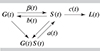 |
Fig. 1. Schematic diagram for nonlinear dynamical exchange (Eqs. (2)–(4)) between gas (G), star (S), and locked-in (L) baryonic matter fractions, regulated by the four potentially time-dependent rates a(t), b(t), c(t), and β(t). |
and
 (4)
(4)
respectively. The spontaneous SFR starts in the truly metal-free primordial gas at the recombination era at z = 1100, during which charged electrons and protons became bound to form electrically neutral hydrogen atoms, so that the gas could decouple from the global expansion and begin to cool efficiently and contract (Klessen & Glover 2023). As initial condition, we adopted
 (5)
(5)
as the whole baryonic gaseous matter was subject to spontaneous star formation. The fact that most star formation only occurs at the centers of overdensities in the large-scale dark matter distribution called dark matter halos can be accounted for by lower values of the coarse-grained averaged rates of spontaneous (β(t)) and triggered (a(t)) star formation.
The initial time t0 corresponds to the redshift z = 1100. The first stars are believed to have formed at z ∼ 30, since prior to z ∼ 30 the gas would not have cooled and grown overdense enough to collapse into stars (Klessen & Glover 2023). Our later results, however, indicated a rather minor influence of the exact starting time of the first stars because we compared with observations at redshifts below z = 8 and hence much smaller than 30 or 1100.
The introduction of gaseous and stellar fractions as the basic dynamical variables has the advantage that the results can be applied to a variety of astrophysical systems (Tinsley 1980) including individual galaxies, clusters of galaxies, and the whole Universe. In each particular case, one has to multiply the derived fractions as a function of time with the respective total mass of baryonic matter.
On the other hand, our approach is simplified as we only considered space-averaged rates for star formation, stellar feedback, and stellar evolution, without accounting for details such as the initial stellar mass function. Of course, these averaged rates can be varied for applications to different astrophysical objects. Our approach is different but bears some similarities with the earlier investigated bathtub (Somerville & Dave 2015) or gas-regulator (Peng & Maiolino 2014) models for galaxy evolution considering the competition among the flow of gas into galaxies, conversion to stars by in situ star formation, and ejection out of galaxies by stellar feedback. This includes individual galaxies, clusters of galaxies, and the whole Universe.
We were particularly interested in the formation rate  of new stars as a function of time:
 (6)
(6)
Obviously, the first term represents the rate from triggered star formation, whereas the second term is the rate from spontaneous star formation.
As mentioned above, we restricted our analysis here to the case of negligible triggered star formation. In this case, exact analytical solutions of the dynamical equations of the GSL model (1)–(5) could be derived. The derived exact analytical solutions hold for stationary rates as well as for the case of the same time dependence of all rates.
3. Negligible triggered star formation
Here, for a(t) = 0, the GSL model Eqs. (2)–(4) simplify to the following linear equations:
 (7)
(7)
 (8)
(8)
and
 (9)
(9)
Introducing the dimensionless time variable
 (10)
(10)
allowed us to eliminate β(t) from the equations and to thus solve them for arbitrary time-dependent rates β(t). Equations (7)–(9) become
 (11a)
(11a)
![Mathematical equation: $$ \begin{aligned} {\mathrm{d}S\over \mathrm{d}\tilde{t}\,}&=G(\tilde{t}\,)-[r_1(\tilde{t}\,)+r_2(\tilde{t}\,)]S(\tilde{t}\,), \end{aligned} $$](/articles/aa/full_html/2024/12/aa51888-24/aa51888-24-eq13.gif) (11b)
(11b)
 (11c)
(11c)
 (11d)
(11d)
with the dimensionless ratios
 (12)
(12)
3.1. Stationary ratios
In the following, we adopted stationary ratios r1= const. and r2= const., so our solution allows for arbitrary but given time-dependent spontaneous rates β(t).
The first equation, (11a) readily provides
![Mathematical equation: $$ \begin{aligned} S(\tilde{t}\,)={1\over r_1}\left[{\mathrm{d}G(\tilde{t}\,)\over \mathrm{d}\tilde{t}\,}+G(\tilde{t}\,)\right] , \end{aligned} $$](/articles/aa/full_html/2024/12/aa51888-24/aa51888-24-eq17.gif) (13)
(13)
which upon insertion into Eq. (11b) yields
 (14)
(14)
Equation (14) is solved by
![Mathematical equation: $$ \begin{aligned} G(\tilde{t}\,)=e^{-\mu \tilde{t}\,}\left[c_-e^{\nu \tilde{t}\,} +c_+e^{-\nu \tilde{t}\,}\right], \end{aligned} $$](/articles/aa/full_html/2024/12/aa51888-24/aa51888-24-eq19.gif) (15)
(15)
with
 (16)
(16)
and with the two integration constants c±, implying the following for Eq. (13)
![Mathematical equation: $$ \begin{aligned} S(\tilde{t}\,)={e^{-\mu \tilde{t}\,}\over r_1}\Bigl [c_-\left(1-\mu +\nu \right)e^{\nu \tilde{t}\,} +c_+\left(1-\mu -\nu \right)e^{-\nu \tilde{t}\,}\Bigr ]. \end{aligned} $$](/articles/aa/full_html/2024/12/aa51888-24/aa51888-24-eq21.gif) (17)
(17)
The initial conditions (5), that is  and
and  provide
 (18)
(18)
so,
 (19)
(19)
The dimensionless formation rate from spontaneous star formation only is given by
![Mathematical equation: $$ \begin{aligned} j(\tilde{t}\,) ={\frac{\mathrm{d}J}{\mathrm{d}\tilde{t}}\;} = G(\tilde{t}\,)=e^{-\mu \tilde{t}\,}\, \left[\cosh (\nu \tilde{t}) -{1-\mu \over \nu }\sinh (\nu \tilde{t}) \right] \end{aligned} $$](/articles/aa/full_html/2024/12/aa51888-24/aa51888-24-eq26.gif) (20)
(20)
and is related to Eq. (6) in this case as  . Consequently,
![Mathematical equation: $$ \begin{aligned} L(\tilde{t}\,) = 1-G(\tilde{t}\,)-S(\tilde{t}\,) = 1-e^{-\mu \tilde{t}\,}\,\left[\cosh (\nu \tilde{t}\,) +{\mu \over \nu }\sinh \left(\nu \tilde{t}\,\right)\right]. \end{aligned} $$](/articles/aa/full_html/2024/12/aa51888-24/aa51888-24-eq28.gif) (21)
(21)
For infinitely large times  we note that
  and
and  , whereas L∞ = 1. While
  and
and  monotonically decrease and increase, respectively, the stellar fraction
  first increases from zero to the maximum value,
 (22)
(22)
at
 (23)
(23)
and the S approaches zero over the course of time: S∞ = 0.
The new star formation rate (6) for the stationary SFR coefficient β0 in this case is
![Mathematical equation: $$ \begin{aligned} \mathring{J} (t)&=\beta _0G(\tilde{t}\,=\beta _0(t-t_0)) \nonumber \\&=\beta _0e^{-\mu \beta _0(t-t_0)}\left[\cosh \left(\nu \beta _0(t-t_0)\right) -{1-\mu \over \nu } \sinh (\nu \beta _0(t-t_0))\right]. \end{aligned} $$](/articles/aa/full_html/2024/12/aa51888-24/aa51888-24-eq37.gif) (24)
(24)
3.2. Negligible stellar feedback
In the special case of negligible stellar feedback b(t) = 0 = r1, one obtains
![Mathematical equation: $$ \begin{aligned} j(\tilde{t}, r_1 = 0)&=G(\tilde{t}, r_1 = 0) \nonumber \\&=e^{-{1+r_2\over 2}\tilde{t}} \left[\cosh {1-r_2\over 2}\tilde{t}\,-\sinh {1-r_2\over 2}\tilde{t}\,\right]=e^{-\tilde{t}\,}, \end{aligned} $$](/articles/aa/full_html/2024/12/aa51888-24/aa51888-24-eq38.gif) (25)
(25)
corresponding to  . Likewise,
 (26)
(26)
and
 (27)
(27)
While  and
and  are monotonically decreasing or increasing, respectively, in this case one finds that
  rises first to the maximum value Smax = r2r2/(1 − r2) at
  and then decreases to the final value of S∞ = 0.
In the special case of r2 = 1, Eqs. (25)–(27) simplify to
 (28)
(28)
Here,  first rises to the maximum value of Smax = e−1 at
  and then decreases to the final value, S∞ = 0.
3.3. Negligible stellar evolution
In the special case of negligible stellar evolution, c(t) = 0 = r2, one obtains
![Mathematical equation: $$ \begin{aligned} j(\tilde{t}, c = 0)=G(\tilde{t}, c = 0)={1\over 1+r_1}\left[r_1+e^{-(1+r_1)\tilde{t}\,}\right], \end{aligned} $$](/articles/aa/full_html/2024/12/aa51888-24/aa51888-24-eq49.gif) (29)
(29)
corresponding to
![Mathematical equation: $$ \begin{aligned} \mathring{J} (t,c = 0)={\beta _0\over b_0+\beta _0}\left[b_0+\beta _0e^{-(b_0+\beta _0)(t-t_0)}\right], \end{aligned} $$](/articles/aa/full_html/2024/12/aa51888-24/aa51888-24-eq50.gif) (30)
(30)
and  . In Fig. 2, we compared the derived exact analytic solutions with the numerical solutions of Eqs. (7)–(9) for several illustrative examples. For the numerical code, we used a single-step solver based on a second-order modified Rosenbrock formula, implemented by Shampine & Reichelt (1997) as ode23s in MatlabTM. The excellent agreement proves the validity of our derivations.
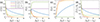 |
Fig. 2. (a) Gas (G), (b) stars (S), and (c) locked-in matter (L) compartments as well as (d) the formation rate |

4. Cosmic star formation history
As an astrophysical application, we considered the present-day (redshift z = 0) gas/star matter ratio and the cosmic star formation history (SFH) of the Universe, which is proportional to the star formation rate (6) as a function of real time. The present-day gas/star matter ratio G(z = 0)/[S(z = 0)+L(z = 0)] = G(z = 0)/[1 − G(z = 0)] in our Milky Way is about 0.1, and a little higher in galaxy clusters. If we take this ratio as characteristic for the whole Universe and allow for a possible contribution of hidden baryons in the intergalactic gas, a value of
 (31)
(31)
seems reasonable (Bland-Hawthorn & Gerhard 2016).
With respect to the cosmic SFH, far-ultraviolet and -infrared measurements have indicated (Madau & Dickinson 2014) that the best-fit SFR density per time t is
![Mathematical equation: $$ \begin{aligned} \psi (z)&={0.015\,(1+z)^{2.7}\over 1+\left[{(1+z)\over 2.9}\right]^{5.6}}\,\mathrm{M}_{\odot }\,\text{ yr}^{-1}\,\text{ Mpc}^{-3} \nonumber \\&={3.22\cdot 10^{-47}\,(1+z)^{2.7}\over 1+\left[{(1+z)\over 2.9}\right]^{5.6}}\,\text{ kg}\,\text{ s}^{-1}\,\text{ m}^{-3}, \end{aligned} $$](/articles/aa/full_html/2024/12/aa51888-24/aa51888-24-eq54.gif) (32)
(32)
where the time t(z) has been expressed as a function of redshift z using a flat ΛCDM Friedmann cosmology (Ryden 2017; Weinberg 2008; Carroll et al. 1992; Peebles 1993), and M⊙ = 1.989 ⋅ 1030 kg in SI-units1. The data used for the best-fit (32) are given in Table 1 of Madau & Dickinson (2014). The SFR density (32) attains its maximum value ψmax = 0.133 M⊙ yr−1 Mpc−3 at redshift z = 1.8632, which is practically constant at small redshifts well below unity, and it decreases at large redshifts ψ(z ≫ 2.9)≃1.25 ⋅ 10−44(1 + z)−2.9 kg s−1 m−3.
Also available in Table 2 and Fig. 11 of Madau & Dickinson (2014) is the integrated stellar density ρ*(z), which according to Madau & Dickinson (2014) fulfills dρ*(z)/dt = (1 − R)ψ(z) and is therefore more explicitly given by
 (33)
(33)
where according to Madau & Dickinson (2014)R is the return factor or the mass fraction of newly born stars; this is put back into the interstellar gas that has been treated as a free fit parameter. As we argue below, within the compartmental model considered here, 1 − R = 1 − L(t(z)) had to be replaced by the time- or redshift-dependent term 1 − L(t) with the fraction L(t) of locked-in stellar matter.
It is worth mentioning earlier works (such as Somerville et al. 2015 and references therein) that have attempted to reproduce the cosmic star formation history and stellar-mass-density evolution jointly with semi-analytic models (see their Fig. 17). The approach followed here is different with respect to the simplicity of the ordinary differential Eqs. (1)–(5), which allowed us to infer analytic constraints (see Sects. 5.1 and 5.2).
4.1. Timescales
We first discuss the relation of our dynamical evolution timescale  for stationary spontaneous SFRs with the look-back time and redshift z in a flat ΛCDM Friedmann cosmology. In a flat ΛCDM Friedmann cosmology with Ωm = Ω0 = 0.3 and H0 = 70 h70 km s−1 Mpc−1 = 2.268 ⋅ 10−18 h70 s−1, the look-back time TL is related to the redshift according to Peebles (1993), Hogg (2000), Boylan-Kolchin & Weisz (2021)
 (34)
(34)
The look-back time TL from now (redshift z = 0) back to redshift z refers to the time that would have elapsed on the clock of an observer moving with the Hubble flow between these redshifts. The look-back time (34) corresponds to the age of the universe T0 given by
 (35)
(35)
The relation between the real time t, the look-back time TL(z), and the age of the Universe T0 is given by
![Mathematical equation: $$ \begin{aligned} t&= T_0-T_L(z)=H_0^{-1}\int _{1+z}^\infty {\mathrm{d}x\over x\sqrt{1-\Omega _0+\Omega _0x^3}} \nonumber \\&={2\over 3\sqrt{1-\Omega _0}H_0} \nonumber \\&\quad \times \ln \left[ {(1+\sqrt{1-\Omega _0})(\sqrt{1-\Omega _0}+\sqrt{1-\Omega _0+\Omega _0(1+z)^3})\over \sqrt{\Omega _0}(1+\sqrt{1-\Omega _0})(1+z)^{3\over 2}}\right], \end{aligned} $$](/articles/aa/full_html/2024/12/aa51888-24/aa51888-24-eq59.gif) (36)
(36)
implying
 (37)
(37)
Consequently,
 (38)
(38)
so, for a constant, spontaneous SFR coefficient β(t) = β0, we obtained
![Mathematical equation: $$ \begin{aligned} \tilde{t}\,(z)&=\beta _0[T_L(1100)-T_L(z)]={2\beta _0\over 3\sqrt{1-\Omega _0}H_0} \nonumber \\&\quad \times \ln \left[{(1101)^{3\over 2}\left(\sqrt{1-\Omega _0}+\sqrt{1-\Omega _0+\Omega _0(1+z)^3}\right)\over (1+z)^{3\over 2}\left(\sqrt{1-\Omega _0}+\sqrt{1-\Omega _0+\Omega _0(1101)^3}\right)}\right] \nonumber \\&={2\beta _0\over 3\sqrt{1-\Omega _0}H_0}\ln \left[\left({1101\over 1+z}\right)^{3\over 2} {1+\sqrt{1+{3\over 7}(1+z)^3}\over 1+\sqrt{1+{3\over 7}(1101)^3}}\right] \nonumber \\& = 3.513\cdot 10^{17}{\beta _0\over h_{70}}\left[0.424+ \ln {1+\sqrt{1+{3\over 7}(1+z)^3}\over (1+z)^{3\over 2}}\right] \text{ s}. \end{aligned} $$](/articles/aa/full_html/2024/12/aa51888-24/aa51888-24-eq62.gif) (39)
(39)
For later use, we note that
 (40)
(40)
with
 (41)
(41)
Accordingly, the reduced time (39) for all values of z is well approximated by
 (42)
(42)
In Fig. 3, we show the variation of Eq. (39) as a function of the redshift z. Obviously, large redshifts correspond to early dynamical times  , whereas small redshifts correspond to late dynamical times. Also shown in Fig. 3 is the approximation (42).
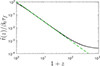 |
Fig. 3. Semi-logarithmic |

In the following two sections, we calculated the SFR density and the stellar density for the case of spontaneous star formation without and with stellar feedback using our results from Sect. 3. We did not consider triggered star formation here. We adopted a flat Universe with Ωtot = 1 so that the critical density would not evolve with redshift and is given by
 (43)
(43)
Consequently, with Ωm = 0.3 the matter density of the Universe is
 (44)
(44)
The matter density (44) includes contributions from dark matter and from baryonic matter, where the latter is a factor 8 smaller than the dark-matter contribution according to Davis et al. (2014). Hence, the baryonic matter density is given by
 (45)
(45)
In general,  is the theoretical cosmic SFR density and the integrated stellar density as a function of redshift,
  , or, equivalently,
 (46)
(46)
with  .
.
Using Eq. (46) thus provides for the integrated stellar mass density according to Eq. (33)
![Mathematical equation: $$ \begin{aligned} \rho _{\rm GSL}^*(z)&= \beta _0^{-1} \int _z^{1100} \mathrm{d}z\prime \,[1-L(z\prime )]\psi _{\rm GS}(z\prime ) \left|{\mathrm{d}\tilde{t}\prime \over \mathrm{d}z\prime }\right| \nonumber \\&\simeq \frac{3}{2} A_1\tau _f \int _z^{1100} \mathrm{d}z\prime \,[1-L(z\prime )] \frac{j(\tilde{t}(z\prime ))}{(1+z\prime )^5} \nonumber \\&= B_1 \int _z^{1100} \mathrm{d}z\prime \, [1-L(z\prime )]\frac{j(\tilde{t}\,(z\prime ))}{(1+z\prime )^5}, \end{aligned} $$](/articles/aa/full_html/2024/12/aa51888-24/aa51888-24-eq76.gif) (47)
(47)
with B1 = 2.24 ⋅ 108β02 kg m−3 and where we have replaced 1 − R = 1 − L(z). This factor enters the calculation of ρGSL*(z), but not the calculation of the SFR density (46) because all stars are born as luminous main-sequence stars. The fraction L(z) resulted from the stellar evolution to locked-in stellar matter, so only the fraction 1 − L(z) contributes to the observed integrated density of luminous stars.
4.2. Observational constraints
In the following sections, we compared the predictions of the GSL model without triggered star formation with the observations. We required the GSL model to be in agreement with the following five observational constraints.
First, the observed peak SFR density has large error bars,
 (48)
(48)
and occurs in the redshift ranges of 1.62–1.88 (Dahlen et al. 2007) and 1.7–2.5 (Cucciati et al. 2012).
Secondly, we required the following observed peak redshift:
 (49)
(49)
As a third constraint, we used the observed integrated stellar mass density at z = 0 (Perez-Gonzalez et al. 2008; Moustakas et al. 2013):
 (50)
(50)
As a fourth constraint, we required (dψ/dz)z = 0 > 0 in order to have at least one maximum of ψ(z) at positive z. As a fifth, more stringent constraint, we required ψGSL(z) to exhibit exactly one maximum within the redshift range z ∈ [0, 8]. While the first to fourth constraints could be dealt with analytically, the fifth constraint was verified by solving a highly nonlinear equation, Eq. (93), numerically.
5. Results for model without stellar evolution
We start with the spontaneous star formation without stellar evolution (a0 = c0 = 0). The omission of stellar evolution is justified as the evolution of most luminous stars occurs on a timescale on the order of the Hubble time (Portinari et al. 1998). We note that for c0 = 0 the fraction (21) of nonluminous locked-in stellar matter vanishes.
5.1. SFR density
We employed the expression (29) for  . With
  from Eq. (42), the SFR density (46) becomes
 (51)
(51)
where we introduced
 (52)
(52)
In terms of
 (53)
(53)
the Eq. (51) reads
 (54)
(54)
The first derivative of the function F(Z) is given by
![Mathematical equation: $$ \begin{aligned} {\mathrm{d}F(Z)\over \mathrm{d}Z}={5\over 3}Z^{2/3}[r_1+(1-0.6\,Z)e^{-Z}], \end{aligned} $$](/articles/aa/full_html/2024/12/aa51888-24/aa51888-24-eq86.gif) (55)
(55)
which is positive for all values of r1 > 0.6 e−5/3 ≈ 0.042, so the function F(Z) has no local extrema in this case.
In order to have a minimum of F(Z), corresponding to an extremum of ψGS(z), the ratio
 (56)
(56)
has to be rather small. For these values of r1, we could already conclude that the gas fraction at infinitely long times,
 (57)
(57)
is below 4%.
Provided restriction (56) holds, two extrema occur at
 (58)
(58)
in terms of the two branches of the Lambert function discussed in Appendix A, where ZE = ϵ0(1 + zE)−3/2. The maximum of ψGS is determined by zE employing the principal branch W0, while W−1 determines the position of the minimum. We had to require that the minimum does not exist for positive redshift values z; that is
 (59)
(59)
corresponding to
 (60)
(60)
which, since r1 > 0, requires ϵ0 > 5/3, or with Eq. (52) that
 (61)
(61)
as first constraint on the value of the spontaneous SFR coefficient β0. The maximum then occurs at the peak redshift:
![Mathematical equation: $$ \begin{aligned} z_E =\left[\frac{5}{3\epsilon _0} - \frac{1}{\epsilon _0}W_0\left(-\frac{5r_1e^{5/3}}{3}\right)\right]^{-2/3} - 1. \end{aligned} $$](/articles/aa/full_html/2024/12/aa51888-24/aa51888-24-eq93.gif) (62)
(62)
For small r1 ≪ 1, the Taylor expansion yielded
 (63)
(63)
The peak SFR density (51) evaluated to
![Mathematical equation: $$ \begin{aligned} \psi _{\rm GS}(z_E)&= {3A_1\over 5(1+r_1)\epsilon _0^{5/3}}Z_E^{8/3}e^{-Z_E} \nonumber \\&=-{A_1r_1\over (1+r_1)\epsilon _0^{5/3}} {\left[{5\over 3}-W_0\left(-\frac{5r_1e^{5/3}}{3}\right)\right]^{8/3} \over W_0\left(-\frac{5r_1e^{5/3}}{3}\right)} \nonumber \\&=-{A_1r_1\epsilon _0\over (1+r_1)W_0\left(-\frac{5r_1e^{5/3}}{3}\right) (1+z_E)^4} \nonumber \\&=-{5.37\cdot 10^{17}A_1r_1\beta _0\,h_{70}^{-1}\over W_0\left(-\frac{5r_1e^{5/3}}{3}\right)(1+z_E)^4} \simeq 1.69\cdot 10^7{\beta _0^3\over (1+z_E)^4} \nonumber \\& = 3.46\cdot 10^{-40}{\beta _0^{1/3}\,h_{70}^{8/3} \over (1+r_1)^{8/3}}\,\text{ kg}\,\text{ s}^{-1}\,\text{ m}^{-3}, \end{aligned} $$](/articles/aa/full_html/2024/12/aa51888-24/aa51888-24-eq95.gif) (64)
(64)
where we used the expansion W0(|x|≪1)≃x and Eq. (63). Equating (64) and (48) yielded
 (65)
(65)
This β0-value2 is partially consistent with the lower limit (61), especially for large values of the observed peak SFR density (48). Consequently, according to Eqs. (52) and (63) we obtained
 (66)
(66)
this large upper limit on zE, however, results from adopting large values of the observed peak SFR density (49) within its large error bars. The upper constraint on zE is consistent with the observational requirement (49).
Consequently, for large values of the observed peak SFR as well as the spontaneous formation rate (65), and values of r1 below the small value (56), the GS model with spontaneous star formation indeed provided a rough but far from optimal fit to the observed SFR density (see Fig. 4).
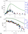 |
Fig. 4. GS model with zero triggered star formation (a0 = c0 = 0) with r1 = 0.001 and |

5.2. Stellar density
Here, we calculated the integrated stellar density for the spontaneous star formation model. With the help of
![Mathematical equation: $$ \begin{aligned} \int ^z \mathrm{d}z\, \frac{e^{-\alpha (1+z)^{-3/2}}}{(1+z)^5} = \frac{2}{3\alpha ^{8/3}} \Gamma \left[\frac{8}{3},\frac{\alpha }{(1+z)^{3/2}}\right], \end{aligned} $$](/articles/aa/full_html/2024/12/aa51888-24/aa51888-24-eq99.gif) (67)
(67)
the integrated stellar mass density (47) with L(z) = 0 becomes
![Mathematical equation: $$ \begin{aligned} \rho ^*_{\rm GS}(z)&= {B_1\over 1+r_1}\int _{z}^{1100} \mathrm{d}z\prime {r_1+e^{-\epsilon _0(1+z\prime )^{-3/2}}\over (1+z\prime )^5} \nonumber \\&={B_1\over 1+r_1}\left({r_1\over 4}\left({1\over (1+z)^4}-1100^{-4}\right) \right.\nonumber \\&\left.\quad + {2\over 3\epsilon _0^{8/3}}\left[\Gamma \left({8\over 3},(1100)^{3/2}\epsilon _0\right)- \Gamma \left({8\over 3},{\epsilon _0\over (1+z)^{3/2}}\right)\right]\right) \nonumber \\&\simeq {2.24\cdot 10^8\beta _0^2\over 4(1+r_1)}\left[{r_1\over (1+z)^4} +{8\over 3}{\gamma \left({8\over 3},{\epsilon _0\over (1+z)^{3/2}}\right)\over \epsilon _0^{8/3}}\right]\,\text{ kg}\,\text{ m}^{-3}, \nonumber \\ \end{aligned} $$](/articles/aa/full_html/2024/12/aa51888-24/aa51888-24-eq100.gif) (68)
(68)
where γ is the lower incomplete gamma function. The stellar mass density thus monotonically decreases from the value
 (69)
(69)
in a power-law fashion at large redshifts z ≫ zE,
 (70)
(70)
since γ(s, ϵ ≪ 1)≃s−1ϵs to the lowest order in ϵ. Equating the result (69) with the observed value (50) provides
 (71)
(71)
where we scaled
 (72)
(72)
in units of 10−17 Hz. The function  is shown in Fig. 5 and varies from 0 to the finite value Γ(8/3)≈1.504 at large arguments. For the nominal values r1 = 0 and h70 = 1, we obtained the following from Eq. (71)
 (73)
(73)
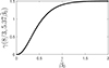 |
Fig. 5. Lower incomplete gamma function, |


which leads to
 (74)
(74)
The two determinations (65) and (74) of the rate of spontaneous star formation, resulting from reproducing the peak value of the SFR density and the present-day integrated stellar mass density within their partially large uncertainties, exclude each other by at a factor of at least 2.8. For example, it is not possible to explain these two constraints with the GS model with one single  value.
Adopting  as a best compromise value, we compared the SFR density and the integrated stellar densities for r1 = 0.001 in Fig. 4. This choice implied zE = 2.46 as peak redshift. Only because of the large error bars in the peak SFR density are the theoretical results of the simplified GS model marginally consistent with the observations. Figure 4 also illustrates the basic dilemma of this simplified model very well. Because of the dependencies
  in Eq. (64) and
  in Eq. (69) on the only free parameter,
  , it is obvious that by decreasing
  from its compromise value 2 would decrease ψGS(z) to smaller values, but it would increase ρGS*(z) at the same time. Alternatively, increasing
  from its compromise value 2 would decrease ρGS*(z) to smaller values, but at the same time it would make ψGS(z) even larger. With the compromise value
  and the ratio r1 = 0.04, the present-day gas fraction is
 (75)
(75)
which is basically identical to the gas fraction at infinite time G∞, and in marginal agreement with the observation (31).
5.3. Special case: Negligible stellar feedback (r1 = 0) and stellar evolution (r2 = 0)
The results of the last subsections included the GS model without stellar feedback (r1 = 0) and stellar evolution (r2 = 0) as a special case. As in this case some of the theoretical results are severely simplified and thus more transparent, we include a detailed analysis of this case here. The SFR density (51) simplified to
 (76)
(76)
with
 (77)
(77)
The density (76) attains its maximum value,
 (78)
(78)
at the peak redshift
 (79)
(79)
The two observational constraints (49) and (48) for zE and the peak SFR density then provided the constraints
 (80)
(80)
and
 (81)
(81)
respectively, which are consistent which each other due to the large uncertainty in the peak SFR density.
The integrated stellar mass density (68) simplifies to
 (82)
(82)
The stellar mass density thus monotonically decreases from the
 (83)
(83)
value in a power-law fashion at large redshifts z ≫ zE,
 (84)
(84)
since  . The estimate (74) for
  from the result (83) with the observed value (50) for the nominal values and h70 = 1 remains unchanged; that is
 (85)
(85)
The two determinations by Eqs. (80), (81), and (85) of the rate of spontaneous star formation, resulting from reproducing the peak redshift and peak value of the SFR density and the present-day integrated stellar mass density within their partially large uncertainties, exclude each other. E.g., it is not possible to explain these three constraints with the simplified GS model using one single  value. Again, a compromise value of
  is suggested. With this compromise value,
  and the present-day gas fraction, in the case of neglected stellar feedback
 (86)
(86)
is another strong disagreement with the observational constraint (31) of this model.
6. SFR and stellar density for spontaneous star formation with stellar feedback
Here, we extended the analysis of the previous section by also including stellar feedback (b0 ≠ 0) besides spontaneous star formation (β0 ≠ 0) and stellar evolution c0 ≠ 0 and using (20), instead of (29) for  .
.
6.1. Theoretical results
With  from Eq. (42) and Eq. (20) for
  the SFR density (46) becomes
![Mathematical equation: $$ \begin{aligned} \psi _{\rm GSL}(z)&= {A_1\over (1+z)^{5/2}} e^{-\mu \tilde{t}\,}\left[\cosh (\nu \tilde{t}) -{1-\mu \over \nu }\sinh (\nu \tilde{t}) \right] \nonumber \\&= {A_1\over \epsilon ^{5/3}}F(\tilde{t}\,), \end{aligned} $$](/articles/aa/full_html/2024/12/aa51888-24/aa51888-24-eq139.gif) (87)
(87)
with μ = (1 + r1 + r2)/2,  ,
,  , as before in Eq. (77), and the function3
![Mathematical equation: $$ \begin{aligned} F(\tilde{t}\,)=\tilde{t}\,^{5/3}e^{-\mu \tilde{t}\,}\left[\cosh (\nu \tilde{t}) +{\mu -1\over \nu }\sinh (\nu \tilde{t}) \right]. \end{aligned} $$](/articles/aa/full_html/2024/12/aa51888-24/aa51888-24-eq142.gif) (88)
(88)
As with Eq. (21), we obtained
![Mathematical equation: $$ \begin{aligned} 1-L(z)=e^{-\mu \tilde{t}\,}\left[\cosh \nu \tilde{t}\,+\, {\mu \over \nu }\sinh \nu \tilde{t}\,\right], \end{aligned} $$](/articles/aa/full_html/2024/12/aa51888-24/aa51888-24-eq143.gif) (89)
(89)
with  . Consequently, the integrated stellar density (47) is given by
![Mathematical equation: $$ \begin{aligned} \rho _{\rm GSL}^*(z)&=B_1\int _z^{1100}\mathrm{d}z\prime \, {e^{-2\mu \tilde{t}\,(z\prime )}\over (1+z\prime )^5} \Bigg [\cosh \nu \tilde{t}\,(z\prime ) \nonumber \\&\quad +{\mu \over \nu }\sinh \nu \tilde{t}\,(z\prime )\Bigg ] \left[\cosh \nu \tilde{t}\,(z\prime )+\, {\mu -1\over \nu }\sinh \nu \tilde{t}\,(z\prime )\right] \nonumber \\&\simeq {B_1\over 6\nu ^2\epsilon ^{8/3}}\int _0^{\epsilon \over (1+z)^{3/2}} \mathrm{d}\tilde{t}\, \tilde{t}\,^{5/3}e^{-2\mu \tilde{t}\,}[(\nu +\mu )e^{\nu \tilde{t}\,}+(\nu -\mu )e^{-\nu \tilde{t}\,}] \nonumber \\&\quad \times [(\nu +\mu -1)e^{\nu \tilde{t}\,}+(\nu +1-\mu )e^{-\nu \tilde{t}\,}] \nonumber \\&={B_1\over 6\nu ^2\epsilon ^{8/3}}\int _0^{\epsilon \over (1+z)^{3/2}} \mathrm{d}\tilde{t}\,\, \tilde{t}\,^{5/3}e^{-2\mu \tilde{t}\,}\left[2(\nu ^2+\mu (1-\mu )) \right.\nonumber \\&\left.\quad +(\nu +\mu )(\nu +\mu -1)e^{2\nu \tilde{t}\,}+(\nu -\mu )(\nu +1-\mu )e^{-2\nu \tilde{t}\,}\right] \nonumber \\&={B_1\over 6\nu ^2(2\epsilon )^{8/3}} \left[{2(\nu ^2+\mu (1-\mu ))\over \mu ^{8/3}}\gamma \left({8\over 3}, {2\mu \epsilon \over (1+z)^{3/2}}\right) \right.\nonumber \\&\quad +{(\nu +\mu )(\nu +\mu -1)\over (\mu -\nu )^{8/3}}\gamma \left({8\over 3},{2(\mu -\nu )\epsilon \over (1+z)^{3/2}}\right) \nonumber \\&\left.\quad +{(\nu -\mu )(\nu +1-\mu )\over (\mu +\nu )^{8/3}}\gamma \left({8\over 3},{2(\mu +\nu )\epsilon \over (1+z)^{3/2}}\right)\right]. \end{aligned} $$](/articles/aa/full_html/2024/12/aa51888-24/aa51888-24-eq145.gif) (90)
(90)
Moreover, the gas fraction (20) as a function of redshift reads
![Mathematical equation: $$ \begin{aligned} G(z)={1\over 2\nu }\left[(\nu +\mu -1)e^{(\nu -\mu )\epsilon \over (1+z)^{3/2}} +(\nu +1-\mu )e^{-{(\nu +\mu )\epsilon \over (1+z)^{3/2}}}\right]. \end{aligned} $$](/articles/aa/full_html/2024/12/aa51888-24/aa51888-24-eq146.gif) (91)
(91)
The first derivative of the function (88) is given by
![Mathematical equation: $$ \begin{aligned} {\mathrm{d}F(\tilde{t}\,)\over \mathrm{d}\tilde{t}\,}&= {\tilde{t}\,^{\,2/3}e^{-\mu \tilde{t}\,}\cosh \nu \tilde{t}\,\over \nu } \Bigg \{{5\over 3}\left[\nu +(\mu -1)\tanh (\nu \tilde{t}) \right] \nonumber \\&\quad +\tilde{t}\,\, \bigl [(\mu -r_2)\tanh (\nu \tilde{t}) -\, \nu \bigr ]\Bigg \}, \end{aligned} $$](/articles/aa/full_html/2024/12/aa51888-24/aa51888-24-eq147.gif) (92)
(92)
so a maximum occurs at  given by the solution of the transcendental equation
![Mathematical equation: $$ \begin{aligned} \left[\nu -(\mu -r_2)\tanh (\nu \tilde{t}_E)\right]\tilde{t}_E ={5\over 3}\left[\nu +(\mu -1)\tanh (\nu \tilde{t}_E)\right]. \end{aligned} $$](/articles/aa/full_html/2024/12/aa51888-24/aa51888-24-eq149.gif) (93)
(93)
As an aside, we note that for r1 = r2 = 0 Eq. (93) correctly reduces to  which is in agreement with Sect. 5.3. Likewise, for r2 = 0 one obtains ν = μ = (1 + r1)/2; with
  and Z defined in Eq. (53), Eq. (93) simplifies to
![Mathematical equation: $$ \begin{aligned} 0.6\,Z\left[1-\tanh {Z\over 2}\right] = 1+r_1+(r_1-1)\tanh {Z\over 2}, \end{aligned} $$](/articles/aa/full_html/2024/12/aa51888-24/aa51888-24-eq152.gif) (94)
(94)
correctly reproducing the determining Eq. (54) with tanh(Z/2) = (1 − e−Z)/(1 + e−Z) for the extrema in the case of negligible stellar feedback.
6.2. Constraints on parameters
First, the observed present-day integrated stellar-mass density (50) provided the following from Eq. (90)
 (95)
(95)
Adopting values of  and assuming |μ − ν|> 0.5, all incomplete γ functions are well approximated by 1.504; so, the constraint (95) simplified to
 (96)
(96)
Secondly, the observed peak redshift (49) yields for
 (97)
(97)
As a third constraint, we inferred the following from Eqs. (48) and (87)
 (98)
(98)
or
![Mathematical equation: $$ \begin{aligned}&0.227^{+0.473}_{-0.056}=\tilde{\beta }_0 ^{1/3}h_{70}^{8/3}F(\tilde{t}_E) =\bigg [\left(1.03^{+0.87}_{-0.36}\right)^{5/3}\tilde{\beta }_0 ^2h_{70} \nonumber \\&\quad \qquad \times \exp \left[-\left(1.03^{+0.87}_{-0.36}\right)\mu \tilde{\beta }_0 h_{70}^{-1}\right] \bigg (\cosh \left(\left(1.03^{+0.87}_{-0.36}\right)\nu \tilde{\beta }_0 h_{70}^{-1}\right) \nonumber \\&\quad \qquad +{\mu -1\over \nu }\sinh \left(\left(1.03^{+0.87}_{-0.36}\right)\nu \tilde{\beta }_0 h_{70}^{-1}\right)\bigg )\bigg ] \end{aligned} $$](/articles/aa/full_html/2024/12/aa51888-24/aa51888-24-eq158.gif) (99)
(99)
with
![Mathematical equation: $$ \begin{aligned} F(\tilde{t}_E)=\tilde{t}_E^{5/3}e^{-\mu \tilde{t}_E}\left[\cosh (\nu \tilde{t}_E)+ {\mu -1\over \nu }\sinh (\nu \tilde{t}_E)\right] \end{aligned} $$](/articles/aa/full_html/2024/12/aa51888-24/aa51888-24-eq159.gif) (100)
(100)
according to Eq. (88), and where we inserted Eq. (97).
As a fourth constraint, we required that (dψ/dz)z = 0 > 0 in order to have a maximum of ψ(z). With
 (101)
(101)
and Eq. (92), one has to require that
![Mathematical equation: $$ \begin{aligned} \nu +(\mu -1)\tanh (\nu \epsilon ) < {3\epsilon \over 5}[\nu -\, (\mu -r_2)\tanh (\nu \epsilon )], \end{aligned} $$](/articles/aa/full_html/2024/12/aa51888-24/aa51888-24-eq161.gif) (102)
(102)
leading, after insertion of Eq. (77), to
 (103)
(103)
6.2.1. Results for standard Hubble constant value h70 = 1
In Fig. 6, we calculated the compatibility of the five constraints on ψGSL(zE), zE, ρGSL*(0), and dψ(z)/dz|z = 0 in the r1–r2-parameter plane over nine decades worth of values each for the wide range of values of ![Mathematical equation: $ \tilde{\beta}_0 \in [0.5,2.7] $](/articles/aa/full_html/2024/12/aa51888-24/aa51888-24-eq163.gif) . Obviously, the tightest constraints on r1 and r2 are provided by the constraints on zE and ρGSL*(0). The green regions on the rightmost panel (labeled summary) for the values of
. Obviously, the tightest constraints on r1 and r2 are provided by the constraints on zE and ρGSL*(0). The green regions on the rightmost panel (labeled summary) for the values of ![Mathematical equation: $ \tilde{\beta}_0 \in[0.9,2.7] $](/articles/aa/full_html/2024/12/aa51888-24/aa51888-24-eq164.gif) indicated the range of parameters r1 and r2, where all five constraints are fulfilled. Although, there is no set of fit parameters
indicated the range of parameters r1 and r2, where all five constraints are fulfilled. Although, there is no set of fit parameters  where all four parameter constraints are fulfilled. This is certainly a significant improvement of the GSL model with spontaneous star formation over the simplified models considered in Sect. 5.
 |
Fig. 6. For each |


![Mathematical equation: $ \tilde{\beta}_0\in[0.9,2.7], $](/articles/aa/full_html/2024/12/aa51888-24/aa51888-24-eq170.gif)
To illustrate this improvement, we compared the redshift dependencies of the SFR density and the integrated stellar density for six different values of  in Fig. 7; this is for all pairs of (r1, r2) values residing either within the green (all five constraints fulfilled for
  ) or within the blue (three constraints fulfilled for
  ) areas of the corresponding panels in Fig. 6. Although the agreement was not perfect for any
  triplet, it was certainly an improvement compared to the model ignoring stellar feedback in Sect. 5. Even with three free parameters, it was still impossible to reproduce the observations nearly perfectly with the GSL model for spontaneous star formation only. Demonstrating that the inclusion of the triggered star formation process can remedy the situation significantly is a challenge for future work.
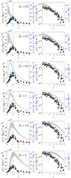 |
Fig. 7. Effect of |


For each of these four  values, we also determined the ranges of the present-day gas fraction from Eq. (91)
![Mathematical equation: $$ \begin{aligned} G(0)={1\over 2\nu }\left[(\nu +\mu -1)e^{(\nu -\mu )\epsilon } +(\nu +1-\mu )e^{-{(\nu +\mu )\epsilon }}\right]. \end{aligned} $$](/articles/aa/full_html/2024/12/aa51888-24/aa51888-24-eq181.gif) (104)
(104)
Using all admissible (r1, r2) pairs, we obtained G(0)∈[0.007, 0.014] for  , G(0)∈[0.0047, 0.0205] for
  , G(0)∈[2.2 × 10⁻⁵, 0.0077] for
  , and G(0)∈[1.48 × 10⁻⁶, 0.0041] for
  . All these values are within a precision level below about 2%.
6.2.2. Smaller values of the Hubble constant
We have previously noticed the strong dependency of the constraints on the adopted value of the Hubble constant with  ,
,  and
and  . Lowering the values of the Hubble constant to values of H0 = 63 km s−1 Mpc−1 or even of H0 = 60 km s−1 Mpc−1 indeed provided better agreement between our theoretical results in Fig. 7 and the observations; that is because in this case ψGLS(zE) and ρGLS(0) are reduced by the factors 0.755 and 0.663, respectively, whereas the peak redshift increases by the factors 1.07 and 1.11, respectively. In Fig. 8, we show the comparison for h70 = 0.857. Lowering the Hubble parameter is, however, not a likely solution as it would lead to violation of other cosmological constraints that we were not considering including the large-scale spatial clustering of galaxies, as reviewed by Wechsler & Tinker (2018).
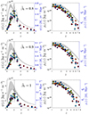 |
Fig. 8. Same as Fig. 7, but for H0 = 60 km s−1 Mpc−1 (corresponding to h70 = 0.857) for |

6.3. Special case of negligible stellar feedback
The general investigation of the case with stellar evolution (r2 > 0) indicated that the special case of negligible stellar evolution (r1 = 0) also meets all constraints. For completeness, we considered this special case here in more detail. We readily found from Eqs. (88) and (89) that
 (105)
(105)
which also holds for r2 = 1, where  . The function
  has a single maximum at
  , so the SFR density ψGLS(z) attains its maximum
 (106)
(106)
at the peak redshift
 (107)
(107)
Consequently,
![Mathematical equation: $$ \begin{aligned} {\psi _{\rm GLS}(z)\over \psi _{\rm GLS}(z_E)} =\left({1+z_E\over 1+z}\right)^{5/2}e^{-\epsilon [(1+z)^{-3/2}-(1+z_E)^{-3/2}]}. \end{aligned} $$](/articles/aa/full_html/2024/12/aa51888-24/aa51888-24-eq196.gif) (108)
(108)
As with μ = (1 + r2)/2 and ν = |1 − r2|/2, in this case Eq. (90) simplifies to
![Mathematical equation: $$ \begin{aligned}&\rho _{\rm GSL}^*(z,r_1 = 0,r_2)={2B_1\over 3(1-r_2)(2\epsilon )^{8/3}}\nonumber \\&\quad \times \left[\left({2\over 1+r_2}\right)^{8/3}\gamma \left({8\over 3}, {(1+r_2)\epsilon \over (1+z)^{3/2}}\right) -r_2\gamma \left({8\over 3},{2\epsilon \over (1+z)^{3/2}}\right)\right]; \end{aligned} $$](/articles/aa/full_html/2024/12/aa51888-24/aa51888-24-eq197.gif) (109)
(109)
in the particular case r2 = 1,
![Mathematical equation: $$ \begin{aligned}&\rho _{\rm GSL}^*(z,r_1 = 0,r_2 = 1)\simeq {2B_1\over 3\epsilon ^{8/3}} \int _0^{\epsilon \over (1+z)^{3/2}}\mathrm{d}\tilde{t}\,\, \tilde{t}\,^{5/3}(1+\tilde{t}\,)e^{-2\tilde{t}\,} \nonumber \\&\quad ={B_1\over 3(2\epsilon )^{8/3}}\left[2\gamma \left({8\over 3}, {2\epsilon \over (1+z)^{3/2}}\right) +\gamma \left({11\over 3}, {2\epsilon \over (1+z)^{3/2}}\right)\right], \end{aligned} $$](/articles/aa/full_html/2024/12/aa51888-24/aa51888-24-eq198.gif) (110)
(110)
while Eqs. (109) and (110) imply, for r2 ≠ 1,
![Mathematical equation: $$ \begin{aligned}&\rho _{\rm GSL}^*(z = 0,r_1 = 0)={2.660\cdot 10^{-29}\,h_{70}^{8/3}\over (1-r_2)\tilde{\beta }_0 ^{2/3}} \nonumber \\&\quad \times \left[\left({2\over 1+r_2}\right)^{8/3}\gamma \left({8\over 3}, 5.37(1+r_2)\right) -r_2\gamma \left({8\over 3},10.74\right)\right] \nonumber \\&\quad \simeq {4.00\cdot 10^{-29}\left[\left({2\over 1+r_2}\right)^{8/3}-r_2\right]h_{70}^{8/3}\over (1-r_2)\tilde{\beta }_0 ^{2/3}}\,\text{ kg}\,\text{ m}^{-3}, \end{aligned} $$](/articles/aa/full_html/2024/12/aa51888-24/aa51888-24-eq199.gif) (111)
(111)
whereas for r2 = 1
 (112)
(112)
here, we approximated both incomplete gamma functions by Γ(8/3) = 1.504 and Γ(11/3) = (8/3)Γ(8/3). We note that with the limit
![Mathematical equation: $$ \begin{aligned} \lim _{r_2\rightarrow 1}{\left[\left({2\over 1+r_2}\right)^{8/3}-r_2\right]\over 1-r_2} =\lim _{x\rightarrow 0}\left[{\left({2\over 2-x}\right)^{8/3}+x-1\over x}\right]={7/3} \end{aligned} $$](/articles/aa/full_html/2024/12/aa51888-24/aa51888-24-eq201.gif) (113)
(113)
one can directly infer Eq. (112) from Eq. (111).
The three constraints (48)–(50) then provided
 (114)
(114)
 (115)
(115)
and
![Mathematical equation: $$ \begin{aligned} \tilde{\beta }_0 =(1.080^{+0.548}_{-0.367})\left[{\left({2\over 1+r_2}\right)^{8/3}-r_2\over 1-r_2}\right]^{3/2}\,h_{70.}^4 \end{aligned} $$](/articles/aa/full_html/2024/12/aa51888-24/aa51888-24-eq204.gif) (116)
(116)
While the first two constraints (114) and (115) restricted the value of  , in Fig. 9 we illustrate the allowed range of values values of the parameters
  and r2 in the case r1 = 0 provided by constraint (116) from the observed ρ*(0).
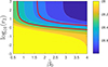 |
Fig. 9. Integrated stellar density (color-encoded) at r1 = 0. Shown is log10[ρGSL*(0) kg−1m3] versus |


For r1 = 0, in the limit r2 → ∞
 (117)
(117)
so  kg m−3. This latter expression agrees with the values for ρGSL(0) shown in Fig. 9 at r2 = 103.
Using Eqs. (25)–(27) and Eq. (42), we obtained the following in the case of negligible stellar feedback for the redshift dependencies of the three fractions:
 (118)
(118)
Adopting the value  for h70 = 1 as the best choice from constraints (114) and (115) thus provided r2 = 6.7 from the third constraint (116). In Fig. 10, we show the redshift dependencies of the three fractions (118) for the parameter set
  . For the present-day values at z = 0, we then found G(z = 0) = 4.67 ⋅ 10−3, S(z = 0) = 8.19 ⋅ 10−4. The vast majority (more than 99.4%) of the baryons in the present Universe reside in the form of locked-in stellar matter in white dwarfs, neutron stars, and black holes.

7. Summary and conclusions
The compartmental description, well known from the description of infectious diseases and epidemics, was applied to describe the temporal evolution of the baryonic matter in interstellar gas and stars. The introduction of gaseous and stellar fractions of the total baryonic matter as the basic dynamical variables was advantageous because it allowed us to apply the description to a variety of astrophysical systems.
In this first paper in a series, the competition of spontaneous star formation, stellar feedback, and stellar evolution was theoretically investigated in order to understand the baryonic matter cycle. The inclusion of the triggered star formation process will be the subject of the second paper of this series. Luminous baryonic matter occurs as interstellar and intergalactic gas with the fraction G(t) as well as in main-sequence stars with the fraction S(t). The third compartment with fraction L(t) denotes weakly luminous matter in white dwarfs, neutron stars, and black holes (referred to as locked-in matter), which have no significant stellar feedback to the gaseous matter compartment. The temporal evolution of the three fractions was controlled by the respective rates of spontaneous star formation (β(t)G(t)), of stellar feedback (b(t)S(t)) of stellar to gaseous matter, and of the formation (c(t)S(t)) of white dwarfs, neutron stars, and black holes from stellar evolution.
When introducing the dimensionless reduced time variable  for an arbitrarily given, time-dependent, spontaneous SFR coefficient β(t), as well as the ratios r1 = b(t)/β(t) and r2 = c(t)/β(t), the derived exact solutions of the dynamical equations hold for stationary rates and for the case of the same time dependence of all rates. The accuracy of the analytical solutions was proven by comparison with the exact numerical solutions of the dynamical equations.
Of particular interest was the understanding of the cosmic star formation history and the present-day gas fraction with compartmental models. For a flat ΛCDM Friedmann cosmology, the relationship between the reduced time variable  and the cosmological redshift z was used to calculate the redshift dependence of the cosmological star formation rate, the integrated stellar density, and the present-day gas fraction from the derived gaseous fraction determining the formation rate of new stars.
A comparison between the observed cosmological star formation rate and the integrated stellar density indicated that the simplified GS model ignoring stellar evolution cannot explain the observations reasonably well with one stationary and spontaneous SFR coefficient β0. The best compromise value β0 = 2.0 ⋅ 10−17 Hz implied a present-day gas fraction in the Universe of about 3.85%.
However, the situation was considerably improved in the full GSL model including stellar evolution, although the agreement with observations is not perfect. Here, the observed cosmological star formation rate and the integrated stellar density as a function of redshift were reasonably well explained by the compartmental model without triggered star formation by the competition of spontaneous star formation and stellar evolution. Conversely, the influence of stellar feedback was less important. The action of stellar evolution provided a significant redshift-dependent reduction factor when calculating the integrated stellar density from the star formation rate. The fits to the observation allowed us to draw conclusions on the relative importance of spontaneous star formation, stellar evolution, and feedback in the early Universe after the recombination era until today.
Lowering the value of the Hubble constant to below the nominal one (h70 = 1) improved the agreement of the GSL model with the observations. The present-day gas, luminous star, and locked-in stellar matter fractions indicated that the vast majority of the baryons (more than 99.4%) reside in the form of locked-in stellar matter in white dwarfs, neutron stars, and black holes. These objects are the astrophysical sites for any hidden baryons. However, both the relatively low value of the Hubble constant and the very high present-day mass fraction in locked-in matter should be interpreted with caution, as they were derived from the still incomplete and imperfect GSL model, which did not account for triggered star formation. The high locked-in matter fraction appeared inconsistent with expectations from stellar evolution models. In these models, for a reasonable choice of the initial mass function (see Kroupa 2001; Chabrier 2003), a stellar population of approximately 13 Gyr has only returned about R= 40% of its originally formed mass to the ISM, with (1 − R)∼60% remaining as surviving stars or remnants. Of that ∼60%, only ∼25% consists of remnants (white dwarfs, black holes, and neutron stars; see Sect. 2.1.2 of the review by Conroy 2013).
The non-perfect agreement of the GSL model with only spontaneous star formation process defines a challenge for future work to demonstrate that the inclusion of the triggered star formation process can remedy the situation significantly. In conclusion, this work has demonstrated that compartmental models of the type introduced here lead to new and original insights on the cosmological baryonic matter cycle in the Universe. The benefit of the proposed compartmental model lies in its simplicity, which enables the derivation of analytical constraints from observations and offers the potential to incorporate additional relevant physical processes.
We note that  .
.
We emphasize the extremely sensitive dependence on the value of the Hubble constant  and also on the ratio r1, as with the upper limit (56) for r1 the factor (1 + r1)8 < 1.39.
To evaluate  for large arguments
  (implying
  ) numerically, one can use
  .
.
Acknowledgments
We are grateful to the anonymous referee for his constructive report that greatly helped to improve the original version of the manuscript. R.S. gratefully acknowledges the institutional support by the Astrophysics Group headed by Prof. Dr. Wolfgang Duschl and Prof. Dr. Sebastian Wolf at the Institut für Theoretische Physik und Astrophysik of the Christian-Albrechts-Universität in Kiel, Germany.
References
- Bland-Hawthorn, J., & Gerhard, O. 2016, ARA&A, 54, 529 [Google Scholar]
- Bonnor, W. B. 1956, MNRAS, 116, 351 [NASA ADS] [CrossRef] [Google Scholar]
- Boylan-Kolchin, M., & Weisz, D. R. 2021, MNRAS, 505, 2764 [NASA ADS] [CrossRef] [Google Scholar]
- Carroll, B. W., & Ostlie, D. A. 2017, An Introduction to Modern Astrophysics 2nd edn. (Cambridge: Cambridge University Press) [Google Scholar]
- Carroll, S. M., Press, W. H., & Turner, E. L. 1992, ARA&A, 30, 499 [NASA ADS] [CrossRef] [Google Scholar]
- Chabrier, G. 2003, PASP, 115, 763 [Google Scholar]
- Clayton, D. D. 1983, Principles of Stellar Evolution and Nucleosynthesis (Chicago: University of Chicago Press) [Google Scholar]
- Conroy, C. 2013, ARA&A, 51, 393 [NASA ADS] [CrossRef] [Google Scholar]
- Cousin, M., Lagache, G., Bethermin, M., & Guiderdoni, B. 2015, A&A, 575, A33 [NASA ADS] [CrossRef] [EDP Sciences] [Google Scholar]
- Cucciati, O., Tresse, L., Ilbert, O., et al. 2012, A&A, 539, A31 [NASA ADS] [CrossRef] [EDP Sciences] [Google Scholar]
- Dahlen, T., Mobasher, B., Dickinson, M., et al. 2007, ApJ, 654, 172 [Google Scholar]
- Dave, R., Finlator, K., & Oppenheimer, B. D. 2011, MNRAS, 416, 1354 [CrossRef] [Google Scholar]
- Davis, A. J., Khochfar, S., & Dalla Vecchia, C. 2014, MNRAS, 443, 985 [NASA ADS] [CrossRef] [Google Scholar]
- Ebert, R. 1955, Z. Astrophys., 37, 215 [NASA ADS] [Google Scholar]
- Elmegreen, B. G. 1997, ApJ, 477, 196 [NASA ADS] [CrossRef] [Google Scholar]
- Estrada, E. 2020, Phys. Rep., 869, 1 [NASA ADS] [CrossRef] [Google Scholar]
- Frank, J., King, A., & Raine, D. 2002, Accretion Power in Astrophysics 3rd edn. (Cambridge: Cambridge University Press) [Google Scholar]
- Hansen, C. J., Kawaler, S. D., & Trimble, V. 2004, Stellar Interiors: Physical Principles, Structure, and Evolution 2nd edn. (New York: Springer) [Google Scholar]
- Hennebelle, P., & Chabrier, G. 2011, ApJ, 743, L29 [Google Scholar]
- Hethcote, H. W. 1989, Biomathematics, 18, 119 [Google Scholar]
- Hethcote, H. W. 2000, SIAM Rev., 42, 599 [CrossRef] [MathSciNet] [Google Scholar]
- Hogg, D. W. 2000, ArXiv e-prints [arXiv:astro-ph/9905116] [Google Scholar]
- Kendall, D. G. 1956, Proceedings of the Third Berkeley Symposium on Mathematical Statistics and Probability (Berkeley: University of California Press) [Google Scholar]
- Kermack, W. O., & McKendrick, A. G. 1927, Proc. R. Soc. A, 115, 700 [Google Scholar]
- Klessen, R. S., & Glover, S. C. 2023, ARA&A, 61, 65 [NASA ADS] [CrossRef] [Google Scholar]
- Kröger, M., & Schlickeiser, R. 2020, J. Phys. A, 53, 505601 [CrossRef] [Google Scholar]
- Kroupa, P. 2001, MNRAS, 322, 231 [NASA ADS] [CrossRef] [Google Scholar]
- Lang, K. R. 1999, Astrophysical Formulae: Space, Time, Matter, and Cosmology 3rd edn. (Berlin: Springer) [CrossRef] [Google Scholar]
- Lang, K. R. 2013, The Life and Death of Stars (Cambridge: Cambridge University Press) [CrossRef] [Google Scholar]
- Low, M. M. M., & Klessen, R. S. 2004, Rev. Mod. Phys., 76, 125 [NASA ADS] [CrossRef] [Google Scholar]
- Madau, P., & Dickinson, M. 2014, ARA&A, 52, 415 [Google Scholar]
- Maoz, D., & Graur, O. 2017, ApJ, 848, 25 [Google Scholar]
- Mercado, F. J., Bullock, J. S., Boylan-Kolchin, M., et al. 2021, MNRAS, 501, 5121 [NASA ADS] [CrossRef] [Google Scholar]
- Moustakas, J., Coil, A. L., Aird, J., et al. 2013, ApJ, 767, 50 [NASA ADS] [CrossRef] [Google Scholar]
- Naoz, S., & Perna, R. 2014, ApJ, 793, L29 [NASA ADS] [CrossRef] [Google Scholar]
- Pandya, V., Fielding, D. B., Bryan, G. L., et al. 2023, ApJ, 956, 118 [NASA ADS] [CrossRef] [Google Scholar]
- Peebles, P. J. E. 1993, Principles of Physical Cosmology (Princeton: Princeton University Press) [Google Scholar]
- Peng, Y., & Maiolino, R. 2014, MNRAS, 443, 3643 [NASA ADS] [CrossRef] [Google Scholar]
- Perez-Gonzalez, P. G., Rieke, G. H., Villar, V., et al. 2008, ApJ, 675, 234 [CrossRef] [Google Scholar]
- Péroux, C., & Howk, J. C. 2020, ARA&A, 58, 363 [CrossRef] [Google Scholar]
- Phillips, A. 1999, The Physics of Stars (Chichester: John Wiley& Sons) [Google Scholar]
- Portinari, L., Chiosi, C., & Bressan, A. 1998, A&A, 334, 505 [NASA ADS] [Google Scholar]
- Ryden, B. 2017, Introduction to Cosmology 2nd edn. (Cambridge: Cambridge University Press) [Google Scholar]
- Sadoun, R., Shlosman, I., Choi, J.-H., & Romano-Diaz, E. 2016, ApJ, 829, 71 [CrossRef] [Google Scholar]
- Shampine, L. F., & Reichelt, M. W. 1997, SIAM J. Sci. Comput., 18, 1 [NASA ADS] [CrossRef] [Google Scholar]
- Shapiro, S. L., & Teukolsky, S. A. 1983, Black Holes, White Dwarfs, and Neutron Stars: The Physics of Compact Objects (New York: Wiley-Interscience) [CrossRef] [Google Scholar]
- Somerville, R. S., & Dave, R. 2015, ARA&A, 53, 51 [NASA ADS] [CrossRef] [Google Scholar]
- Somerville, R. S., Popping, G., & Trager, S. C. 2015, MNRAS, 453, 4337 [Google Scholar]
- Tielens, A. G. G. M. 2005, The Physics and Chemistry of the Interstellar Medium (Cambridge: Cambridge University Press) [Google Scholar]
- Tinsley, B. M. 1980, Fundament. Cosmic Phys., 5, 287 [NASA ADS] [Google Scholar]
- Tortora, C., Hunt, L. K., & Ginolfi, M. 2022, A&A, 657, A19 [NASA ADS] [CrossRef] [EDP Sciences] [Google Scholar]
- Tumlinson, J., Peeples, M. S., & Werk, J. K. 2017, ARA&A, 55, 389 [Google Scholar]
- Wechsler, R. H., & Tinker, J. L. 2018, ARA&A, 56, 435 [NASA ADS] [CrossRef] [Google Scholar]
- Weinberg, S. 2008, Cosmology (Oxford: Oxford University Press) [Google Scholar]
- Woosley, S. E., & Janka, H.-T. 2005, Nat. Phys., 1, 147 [NASA ADS] [CrossRef] [Google Scholar]
Appendix A: Lambert functions
In this manuscript we encountered transcendental equations of the form
 (A.1)
(A.1)
with arbitrary values of A and C. Substituting y = e−x then yields for Eq. (A.1)
 (A.2)
(A.2)
which can be solved (see Appendix G in Kröger & Schlickeiser (2020)) as
 (A.3)
(A.3)
in terms of Lambert functions. Consequently, the solution of Eq. (A.1) is given by
 (A.4)
(A.4)
where we used Lambert’s equation
 (A.5)
(A.5)
defining the Lambert function W(z). The Lambert equation (A.5) can only be solved for real-valued z if z ≥ −1/e. One obtains the principal branch W0(z) for arguments z ≥ 0 and the two branches W0(z) and W−1(z) if −1/e ≤ z ≤ 0. For these negative real arguments the principal branch has values W0(z)∈[−1, 0] and the lower branch W−1(z) < − 1 has values smaller than −1.
All Figures
|
Fig. 1. Schematic diagram for nonlinear dynamical exchange (Eqs. (2)–(4)) between gas (G), star (S), and locked-in (L) baryonic matter fractions, regulated by the four potentially time-dependent rates a(t), b(t), c(t), and β(t). |
| In the text | |
|
Fig. 2. (a) Gas (G), (b) stars (S), and (c) locked-in matter (L) compartments as well as (d) the formation rate |
| In the text | |
|
Fig. 3. Semi-logarithmic |
| In the text | |
|
Fig. 4. GS model with zero triggered star formation (a0 = c0 = 0) with r1 = 0.001 and |
| In the text | |
|
Fig. 5. Lower incomplete gamma function, |
| In the text | |
|
Fig. 6. For each |
| In the text | |
|
Fig. 7. Effect of |
| In the text | |
|
Fig. 8. Same as Fig. 7, but for H0 = 60 km s−1 Mpc−1 (corresponding to h70 = 0.857) for |
| In the text | |
|
Fig. 9. Integrated stellar density (color-encoded) at r1 = 0. Shown is log10[ρGSL*(0) kg−1m3] versus |
| In the text | |
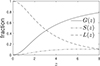 |
Fig. 10. G(z), S(z), and L(z) for r1 = 0, r2 = 6.7, and |
| In the text | |
Current usage metrics show cumulative count of Article Views (full-text article views including HTML views, PDF and ePub downloads, according to the available data) and Abstracts Views on Vision4Press platform.
Data correspond to usage on the plateform after 2015. The current usage metrics is available 48-96 hours after online publication and is updated daily on week days.
Initial download of the metrics may take a while.