| Issue |
A&A
Volume 692, December 2024
|
|
|---|---|---|
| Article Number | A153 | |
| Number of page(s) | 13 | |
| Section | Astrophysical processes | |
| DOI | https://doi.org/10.1051/0004-6361/202451568 | |
| Published online | 09 December 2024 | |
Thermal solutions of strongly magnetized disks and the hysteresis in X-ray binaries
1
Univ. Grenoble Alpes, CNRS, IPAG, 38000 Grenoble, France
2
School of Physics and Astronomy, University of Southampton, Highfield, Southampton, SO17 1BJ, UK
3
JILA, University of Colorado and National Institute of Standards and Technology, 440 UCB, Boulder, CO, 80309-0440, USA
4
Department of Astrophysial and Planetary Sciences, University of Colorado, 391 UCB, Boulder, CO, 80309-0391, USA
5
Institute of Astronomy, University of Cambridge, Madingley Road, Cambridge, CB3 OHA, UK
6
Nicolaus Copernicus Astronomical Center, Polish Academy of Sciences, Bartycka 18, PL-00-716 Warszawa, Poland
⋆ Corresponding author; This email address is being protected from spambots. You need JavaScript enabled to view it.
Received:
18
July
2024
Accepted:
11
October
2024
Abstract
Context. X-ray binaries (XRBs) exhibit a spectral hysteresis for luminosities in the range 10−2 ≲ L/LEdd ≲ 0.3, with a hard X-ray spectral state that persists from quiescent luminosities up to ≳0.3LEdd, transitioning to a soft spectral state that survives with decreasing luminosities down to ∼10−2LEdd.
Aims. We present a possible approach to explain this behavior based on the thermal properties of a magnetically arrested disk simulation.
Methods. By post-processing the simulation to include radiative effects, we solved for all the thermal equilibrium solutions as the accretion rate, Ṁ, varies during the XRB outburst.
Results. For an assumed scaling of the disk scale height and accretion speed with temperature, we find that two solutions exist in the range of 10−3 ≲ Ṁ/ṀEddington ≲ 0.1 at r = 8 rg (4 × 10⁻² ≲ Ṁ/ṀEddington ≲ 0.5 at r = 3 rg): a cold, optically thick solution, and a hot, optically thin one. This opens the possibility of a natural thermal hysteresis in the right range of luminosities for XRBs. We stress that our scenario for the hysteresis does not require us to invoke the strong advection-dominated accretion flow principle, nor does it require the magnetization of the disk to change during the XRB outburst. In fact, our scenario requires a highly magnetized disk in the cold soft state to reproduce the transition from soft to hard state at the right luminosities. Our scenario therefore predicts a jet, although possibly very weakly dissipative, in the soft state of XRBs. We also predict that if active galactic nuclei have similar hysteresis cycles and are strongly magnetized, they undergo a transition from soft to hard state at much lower L/LEdd than XRBs.
Key words: accretion / accretion disks / magnetohydrodynamics (MHD) / stars: black holes / galaxies: active / X-rays: binaries
© The Authors 2024
 Open Access article, published by EDP Sciences, under the terms of the Creative Commons Attribution License (https://creativecommons.org/licenses/by/4.0), which permits unrestricted use, distribution, and reproduction in any medium, provided the original work is properly cited.
This article is published in open access under the Subscribe to Open model. This email address is being protected from spambots. You need JavaScript enabled to view it. to support open access publication.
1. Introduction
X-ray binaries (XRBs) are compact binary systems containing a stellar-mass black hole or a neutron star that accretes from a stellar companion through an accretion disk. A large fraction of XRBs has outburst cycles during which their bolometric luminosities rise by several orders of magnitudes above the quiescent level (Dunn et al. 2010; Tetarenko et al. 2016). These outbursts last from weeks to years, and they usually recur on periods of years to decades (see Done et al. 2007, for a compilation of lightcurves of XRBs).
One of the most intriguing aspects of XRBs is that they change spectral state during their outburst, with the hardness ratio (the ratio of hard to soft X-rays) forming a hysteresis cycle (Dunn et al. 2010). For simplicity, we define two states: the soft state, and the hard state (Remillard & McClintock 2006). Schematically, XRBs start in quiescence in a hard state in which they remain up to luminosities of ≳30% of the Eddington luminosity before switching to the soft state (but see failed-transition outbursts; Alabarta et al. 2021). On their return to quiescence, XRBs stay in the soft state down to luminosities of ∼1% of the Eddington luminosity before switching back to a hard state and down to quiescence (Maccarone 2003). The hysteresis appears between 1% and ≳30% of the Eddington luminosity, where XRBs can be found in two different spectral states, depending on whether they are on their way up or down in luminosity (Dunn et al. 2010).
The soft state is dominated by thermal emission that peaks around 1 keV, while the hard state is a power-law-dominated state with a hard to inverted photon spectral index Γ ∼ 2.1 to 1.6 and a cutoff around 100 keV. In both states, a subdominant high-energy power-law tail extending to the MeV can be observed (Grove et al. 1998; Laurent et al. 2011; Jourdain et al. 2012; Cangemi et al. 2023). The usual interpretation of the soft state is that it originates from a relatively cold (≈107 K), optically thick disk that radiates as a multitemperature blackbody (Shakura & Sunyaev 1973; hereafter SS73). Since the SS73 model is valid in a very extended regime of accretion rates that extends from almost-Eddington sources to highly sub-Eddington sources, it is unclear why XRBs below 1% of the Eddington luminosity are never observed to be in a soft state (see Shaw et al. 2016 for the few known soft-to-hard state transitions at lower luminosities). The usual interpretation of the hard state is that it originates from hot (≈109 K), optically thin gas in which hot electrons scatter low-energy photons up to high energies by the inverse-Compton process and produce a power-law spectrum via multiple scattering (Sunyaev & Titarchuk 1980). Finally, the origin of the high-energy power-law tail that extends to the MeV regime is more strongly debated, but is usually thought to involve nonthermal electrons that are accelerated in a jet (Zdziarski et al. 2012) or in a hot region around the black hole, such as the plunging region (Hankla et al. 2022).
Although most models agree that the hard X-ray emission that peaks at 100 keV originates from a hot, optically thin component, called a hot corona (but see Sridhar et al. 2021; Grošelj et al. 2024 for simulations showing the formation of a cold corona), the physical nature of this hot corona is still under debate. At a low luminosity, where the electrons and protons are decoupled, it is now accepted that the hot corona can be associated with the entire accretion flow, that is, a hot, two-temperature, geometrically thick flow (Narayan 1996; Esin et al. 1997; Petrucci et al. 2010; Poutanen & Veledina 2014; Marcel et al. 2018a; Dexter et al. 2021). However, at high luminosities, analytical calculations and numerical simulations both predict that a hot accretion flow thermally collapses when the electrons become well coupled to the protons (Yuan & Narayan 2014; Dexter et al. 2021), leading to speculation regarding the nature and geometry of the hot X-ray corona at high luminosities. Two different geometries have been debated in the community: (1) A vertically extended geometry, such as the lamppost model, in which the corona is a compact source above the black hole (Matt et al. 1991; Martocchia & Matt 1996; Henri & Petrucci 1997; Dauser et al. 2013) that might be associated with an X-ray emitting jet (Markoff et al. 2005), or (2) a horizontally extended geometry, in which the hot corona replaces or truncates the inner geometrically thin, optically thick disk in the innermost parts of XRBs (Haardt et al. 1994; Ferreira et al. 2006; Schnittman et al. 2013; Marcel et al. 2018a; Kinch et al. 2021). However, recent measurements of the X-ray polarization angle by the Imaging X-ray Polarimetry Explorer mission (IXPE) have mostly settled this debate by showing that the polarization angle is perpendicular to the disk. This strongly favors models in which the corona is located in the disk plane (Krawczynski et al. 2022)1.
To form a horizontal corona that effectively replaces the inner optically thick disk in XRBs is no trivial task at high luminosities. Because the density in a hot accretion flow increases with luminosity, we expect a hot accretion flow to thermally collapse around L ≈ 10−2LEdd (Esin et al. 1997; Yuan & Narayan 2014). The two main scenarios for maintaining a hot inner flow at high densities either rely on the evaporation of the thin disk by a hot atmosphere (Meyer & Meyer-Hofmeister 1994; Spruit & Deufel 2002) or on a highly magnetized disk (Ferreira et al. 2006; Petrucci et al. 2010; Oda et al. 2012; Cao 2016; Marcel et al. 2018a,b, 2019). The evaporation scenario has recently been disfavored by shearing-box simulations (Bambic et al. 2024), while the high-magnetization scenario has been highly successful in explaining the phenomenology of XRBs (Marcel et al. 2018a,b). We focus on the magnetic scenario in the remainder of this paper.
The main idea behind all strongly magnetized models (see Sect. 2 for a quantitative definition of highly magnetized disks) is that strong magnetic fields enhance the radial speed of the accretion flow and its density scale height (Ferreira & Pelletier 1995; Ferreira et al. 2006; Oda et al. 2012; Scepi et al. 2024). This is true in self-similar solutions for the jet-emitting disk (JED; Ferreira & Pelletier 1995) and in general relativistic magneto-hydrodynamic (GRMHD) simulations of magnetically arrested disks (MAD; Scepi et al. 2024, hereafter referred to as SBD24). As a consequence, the density for a given accretion rate is lower in a strongly magnetized disk than in a weakly magnetized disk, which pushes hot, optically thin solutions to higher luminosities. This opens up the possibility that a hot, hard X-ray corona forms at high luminosities in XRBs (Ferreira et al. 2006; Petrucci et al. 2010; Oda et al. 2012; Cao 2016; Marcel et al. 2018a; Liska et al. 2022).
Moreover, the magnetization provides a second parameter, with the accretion rate, to produce a hysteresis cycle. Several authors have suggested that the transitions between the XRB spectral states are caused by sudden changes in the magnetization of the accretion flow (Ferreira et al. 2006; Petrucci et al. 2008; Igumenshchev 2009; Begelman & Armitage 2014; Cao 2016; Marcel et al. 2019). When the accretion flow is highly magnetized, it forms a hot corona (a hard spectral state), and when the accretion flow is weakly magnetized, it forms a cold, optically thick disk (a soft spectral state). This idea is supported by the fact that the compact radio emission that is observed in the hard state, which is usually associated with the presence of a magnetic jet, is quenched during the transition to the soft state (Fender et al. 2004, 2009; Corbel et al. 2012; but see Drappeau et al. 2017; Péault et al. 2019). However, we still lack an understanding of the mechanisms that could drive these magnetization changes. Most notably, there is no understanding of why the soft-to-hard transition occurs at almost the same luminosity in all XRBs if it is driven by a change in magnetization.
Following another approach, Marcel et al. (2018a) has investigated a scenario in which the hysteresis of XRBs could be a thermal instead of a magnetic hysteresis. In their scenario, a high-magnetization disk is present throughout the hysteresis cycle, so that there is no need for unknown mechanisms to drive the magnetization changes. However, the authors reported that a thermal hysteresis can only be formed in strongly magnetized disks in the range 10−4 ≲ L/LEdd ≲ 10−2. This is too low by at least an order of magnitude to explain the phenomenology of XRBs. Recently, SBD24 have shown that GRMHD simulations of thin MAD disks share many properties with JED semi-analytical solutions, but differ in several respects, namely in the magnetic support in the vertical direction (but see Zimniak et al. 2024) and in the higher radiative efficiency of the disk. These properties of MADs might be able to push the thermal hysteresis to higher luminosities, and this motivated us to revisit the scenario of Marcel et al. (2018a) in the present paper.
Our paper is structured as follows. In Sect. 2, we summarize the dynamical results of the GRMHD MAD simulation from SBD24. In Sect. 3, we post-process the simulation of SBD24 to include the cooling mechanisms and investigate the thermal structure of the hard state. In Sect. 4, we extrapolate the thermal solutions of the thin MAD simulation to the soft state, discuss the presence of thermal hysteresis, and compare it to the hysteresis found in JED semi-analytical solutions. At the end of Sect. 4, we also extrapolate our scenario to the case of active galactic nuclei (AGN) and discuss the possible presence of a jet in the soft state of XRBs.
2. Dynamical properties of strongly magnetized disks
We refer to strongly magnetized disks as disks with a magnetic field that is of dynamical importance, or more quantitatively, as disks with a large-scale vertical field, Bz, such that βz, mid ≡ 2(pgas + prad)/Bz, lam2(z = 0) is ≲100. Here, pgas, prad, and Bz, lam are the gas pressure, radiation pressure, and laminar vertical field, respectively. Although a vertical field with βz, mid ≈ 100 is not dynamically important by itself, it establishes other field components (both turbulent and laminar) through the action of the magneto-rotational instability and of magnetic winds that are dynamically important. Hence, we stress the importance of defining strongly magnetized disks with the βz, mid parameter and not with the β parameter, which includes all the other components (Jacquemin-Ide et al. 2021). Because the net magnetic flux cannot be desctructed, Bz can be regarded as a control parameter of the system, whereas the other field components are an outcome of physical mechanisms depending on Bz. Our definition of strongly magnetized disks includes both JED semi-analytical solutions and MAD numerical simulations, which share many dynamical properties (Scepi et al. 2024).
We post-processed the results of the GRMHD simulation of a thin MAD disk by SBD24. The simulation was performed with the code ATHENA++ (White et al. 2016; Stone et al. 2020) using Kerr-Schild coordinates and was initialized with a Fishbone & Moncrief (1976) torus with an inner radius of 16.45 rg and a pressure maximum at 34 rg, where rg ≡ GMBH/c2 is the gravitational radius, G is the gravitational constant, MBH is the mass of the black hole, and c is the speed of light. The black hole spin is a = 0.9375, and the βz, mid parameter is ≈100 throughout the initial torus. The effective resolution is 1024 × 512 × 1024 (four levels of static mesh refinement were used) for a domain of size [1.125 rg, 1500 rg],[0, π],[0, 2π] in the r, θ, and ϕ directions, respectively. A snapshot of the simulation at 40 400 rg/c was used for our analysis. We also used time-averaged and ϕ-averaged data from SBD24 for the heating rate2 in Sect. 3 and for all quantities in Sect. 4. We always used a time- and ϕ-averaged version of the heating rate because it is a noisy quantity. Time averages were made between 40 000 and 41 000 rg/c to isolate a local moment in time around our snapshot while having good statistics on the heating rate. We also tried the same averaging window as in SBD24, that is, between 40 000 and 44 000 rg/c, and did not find any substantial difference in our results.
To obtain a thin disk, SBD24 used an artificial cooling function to cool the disk to a targeted thermal scale height of hth/r = 0.03, where
 (1)
(1)
cs is the sound speed in the midplane, and vK is the relativistic Keplerian velocity around a Kerr black hole, defined as in Noble et al. (2009). The disk eventually became a thin MAD (Igumenshchev 2008), with βz, mid ≈ 26 when averaged over r < 10 rg (see Fig. 1) and a β parameter (also in the midplane, but including all field components) ≈0.2, so that magnetic effects dominated the dynamics of the disk.
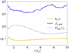 |
Fig. 1. Radial profiles of the geometrical density scale height (solid gold line), the βz, mid in the midplane (solid blue line) and the density-weighted radial three-vector velocity normalized by the sound speed (dashed gray line). The density scale height and the radial speed exceed expectations from standard theory. |
The dominance of the magnetic field causes the dynamical disk properties to diverge from standard theory in the following respects:
-
1.
The vertical structure is supported by the gradient of the turbulent magnetic pressure in the disk, not by the gradient of thermal pressure, as in SS73. Indeed, we plot in the top panel of Fig. 1 the geometrical scale height of the disk,
 (2)
(2)where
 as in McKinney et al. (2012). We find that hρ/r ≈ 0.09 for hth/r = 0.03, so that the geometrical scale height is three times larger than the thermal scale height.
 -
2.
The accretion is mostly due to large-scale magnetic stress originating from a magnetized wind (Blandford & Payne 1982; Ferreira & Pelletier 1993), not to viscous stress, as in SS73. As a result, the accretion speed is much higher than in standard theory, as was also found in JED solutions (Ferreira & Pelletier 1995; Ferreira 1997). This is shown in the bottom panel of Fig. 1, where we plot the accretion speed normalized by the sound speed,
 , where V is the three-vector velocity. We find vr/cs ≈ 0.8 when averaged over r < 10 rg, which can be compared with a prediction of 3 × 10⁻² for α = 1 in standard theory.
 -
3.
The dissipation profile does not follow the thermal pressure latitudinal profile, as in SS73, because it shows significant dissipation at the base of the wind. This is shown in Fig. 2, where we plot the ratio contours of the cumulative heating rate in the latitudinal direction up to θ to the cumulative heating rate in the latitudinal direction up to ∞. Less than 30% of the dissipation occurs within z/r ± 0.03 (i.e., z/hth ± 1).
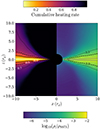
Fig. 2. Right panel: Time- and ϕ-averaged log of the density in the simulation of SBD24, normalized by the density in the midplane that would be obtained from the SS73 model with the same accretion rate, with α = 1 and hth/r = 0.03. The black lines show three contours of the color map. The gray lines show the surfaces of z/r = ±0.03. Left panel: Time- and ϕ-averaged cumulative heating rate, i.e., the ratio of the heating rate latitudinally integrated up to θ to the heating rate latitudinally integrated up to ∞. The black lines show three contours of the cumulative heating rate.
-
4.
There is a significant amount of heating inside the innermost stable circular orbit (ISCO) (Agol & Krolik 2000), which provides additional dissipation compared to the model of SS73.
An important consequence of magnetic support and wind-driven accretion is that the disk is much less dense than expected in standard theory (Ferreira et al. 2006). This is shown in Fig. 2, where the right panel shows the density in the SBD24 simulation, divided by the expected density in standard theory if the disk were accreting at the same accretion rate with α = 1. Even in the midplane, the disk density is three orders of magnitude lower than expected. Moreover, the density slope in the MAD simulation is very shallow. It scales as ∝r−1 compared to ∝r−15/8 in standard theory. This is the slope expected in a JED with an ejection index of ≈0.5, such as in SBD24, which once again shows the similarity between JED semi-analytical solutions and MAD numerical simulations. Finally, we stress that the low densities of strongly magnetized disks, coupled to the nonzero magnetic stress at the ISCO in the MAD simulation, enable the formation of a hot coronal state at high accretion rates, as we describe in the next section.
3. Post-processing of the hard state
3.1. Post-processing procedure
In this section, we post-process the simulation of SBD24 to solve for the gas temperature. We assumed that ions and electrons are well coupled so that the plasma has only one temperature. We discuss this assumption later on in this section. We also neglected feedback of thermal pressure and radiation pressure on the dynamical structure of the disk. This choice is motivated by the dominance of magnetic effects over thermal effects in setting the dynamical structure of the strongly magnetized disk in SBD24. This neglect of thermal feedback is likely to hold as long as the final post-processed temperature does not depart too much from the targeted temperature used in SBD24 (see Sect. 4, when we impose large deviations). As the targeted thermal scale height of hth/r = 0.03 used in SBD24 sets a temperature between 108 and 109 K in the inner 10 rg of an X-ray binary, this makes our post-processing particularly relevant to the study of the hot coronal hard spectral state. However, we note that in the cold solutions discussed in Section 4, where the departure from the targeted thermal scale height of hth/r = 0.03 is large, the radiation pressure starts to dominate the magnetic pressure for ṁ > 10−2, so that the disk structure is expected to be altered by the radiative effects in this case. It is beyond the scope of this paper to take these effects into account.
To solve for the gas temperature, we equated the fluid-frame heating rate per unit of proper time and volume as defined and measured in SBD24, qheat, with a cooling rate that we estimated in post-processing, qcool, following Esin et al. (1996). The heating rate is a measure of the amount of internal energy that was removed to keep a constant temperature in the disk in the simulation of SBD24. Hence, it also takes heat advection into account.
To compute the cooling rates, we made a few assumptions. We neglected bound-free and bound-bound cooling processes as the plasma in XRBs is expected to be highly ionized. We also neglected external Compton cooling, which was found to be subdominant at high luminosities (≈10%LEdd) in the JED solution of Marcel et al. (2018b) 3. This means that we only considered synchrotron self-Compton, denoted as qsynch, C, and bremsstrahlung self-Compton emission, denoted as qbrem, C, with the formulas taken from Esin et al. (1996). Hence, the cooling rate in the optically thin regime, which is purely local, is given by
 (3)
(3)
At large optical depths, we also take blackbody emission into account, given by
 (4)
(4)
where Te is the electron temperature. Here, τtot is a local estimate of the total optical depth,
 (5)
(5)
where κR = 5 × 1024ρT−3.5g cm−2 is the Rosseland mean opacity, and κes is the electron-scattering opacity4. Finally, we made the transition from the optically thin to the optically thick regime by using the bridge formula from Artemova et al. (1996),
![Mathematical equation: $$ \begin{aligned} q_{\rm cool} = q_{\rm thick}\left(1+\frac{4}{3 \tau _{\rm tot}}\left[1+\frac{1}{2\tau _{\rm abs}}\right]\right)^{-1} \end{aligned} $$](/articles/aa/full_html/2024/12/aa51568-24/aa51568-24-eq8.gif) (6)
(6)
where we defined the optical depth to absorption as
 (7)
(7)
It can easily be verified that in the effectively optically thin regime, when τabs ≪ 1 and  , Eq. (6) tends to qthin, while in the optically thick regime, when τabs ≫ 1 and τtot ≫ 1, Eq. (6) tends to qthick (Artemova et al. 1996).
The density in the ideal MHD simulation of SBD24 is a dimensionless parameter, which we converted into physical units using
 (8)
(8)
where Munit = ṀXRB/Ṁcode × tunit, Vunit ≡ (GMBH/c2)3, and tunit ≡ GMBH/c3. Here, ṀXRB, Ṁcode, and MBH are the accretion rate in cgs units, the accretion rate in code units from the simulation of SBD24, and the mass of the central black hole in cgs units, respectively. In the following, we use MXRB = 10M⊙ and ṁ = ṀXRB/ṀEdd, with ṀEddc2 ≡ LEdd/0.1, to set the accretion rate.
To summarize, in order to find the temperature in post-processing, we solved the following equation:
 (9)
(9)
where the choice of a black hole mass and an accretion rate sets the physical units of ρ and of the magnetic field, B.
3.2. Temperatures in the hard state
Figs. 3 and 4 show a poloidal cut and a midplane cut, respectively, of the post-processed temperature for different accretion rates. In the poloidal cut, we exclude the jet region (defined here as where the cold magnetization σ ≡ B2/ρ exceeds unity) from our analysis.
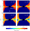 |
Fig. 3. Poloidal cuts of the post-processed temperature for four different accretion rates. The jet region (defined as the region where σ > 1) is excluded from our analysis. |
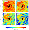 |
Fig. 4. Midplane cut of the post-processed temperature for four different accretion rates. The temperature is inhomogeneous, but even at high accretion rates, patches of hot gas can survive. |
In all cases, we find that a significant fraction of the gas can stay hot, even at high accretion rates. For example, for ṁ = 0.3, ≈75% of the heat is dissipated in regions with temperatures above 108 K. The averaged temperature weighted by qheat evolves from ≈1010 K for ṁ = 0.01 to ≈109 K for ṁ = 0.3. We note that the high-temperature region in the left corner of the panels of Fig. 4 is related to the presence of a previous MAD eruption (see Igumenshchev 2009; McKinney et al. 2012 for literature on the MAD eruptions). This region has a relatively low density, high magnetization, and is typically dominated by synchrotron self-Compton emission (see Fig. B.2). Remnants of MAD eruptions are present at any given time within 10 rg, so that these eruptions might play a large role in producing high-temperature spots in the inner disk.
We also plot in Fig. 5 the yC Compton parameter in the nonrelativistic limit,
 (10)
(10)
The averaged yC weighted by qheat evolves from ≈0.8 at ṁ = 0.01 to ≈20 for ṁ = 0.3, so that a relatively hard spectral index is expected from a spectral post-processing of our simulations.
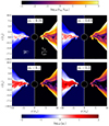 |
Fig. 5. Poloidal cut of the yC Compton parameter and the ratio of the electron-proton collision time to the advection time. |
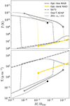 |
Fig. 6. Thermal solutions of the MAD numerical simulation at r = 8 rg for an XRB with MBH = 10 M⊙. In both panels, the gray line shows the hot, optically thin branch that extends up to ṁ ≈ 10−1, while the gold line shows the cold, optically thick branch that only extends down to ṁ ≈ 10−3. The black lines show reference solutions for comparison with the dash-dotted, dotted, and dashed lines, which show the solutions for a standard Shakura-Sunyaev disk, a one-temperature ADAF analytical solution, and a two-temperature JED semi-analytical solution, respectively. The uniqueness of our MAD thermal solutions is that they have two stable thermal branches within the range 10−3 ≲ ṁ ≲ 10−1. |
We also note the presence of localized dense clumps with temperatures of ≈106 − 7 in the body of the disk, which cool down through blackbody emission (as shown in Figs. B.1 and B.2). These clumps appear in the outer disk at a low accretion rate and spread to the inner disk as the accretion rate increases. This is reminiscent of the clumps reported in Liska et al. (2022). These cold clumps could cool the surrounding hot gas by external Compton scattering, an effect that we neglect here. However, these clumps are also embedded in hot gas, and so it remains to be seen whether they can survive when irradiated by the surrounding hard radiation.
By averaging over time and ϕ, we computed the density-weighted temperature as a function of radius and defined a truncation radius, that is, a radius within which the disk is hotter than 108 K. We find that for ṁ = 0.01, this radius is > 10 rg (i.e., beyond our analysis radius), while for ṁ = 0.3, this radius is ≈7 rg. The truncation thus naturally recedes inward as ṁ increases. We emphasize that the truncation radius does not recede inward because of a change in the magnetization of the disk. In our normalization procedure, we assumed that the magnetization stays the same for all ṁ. The truncation radius simply traces the radius at which the disk can no longer stay hot because the cooling rate would otherwise exceed the heating rate. The fact that the truncation radius appears in the outer part and propagates inward follows from the shallowness of the density profile in SBD24. As the density is relatively shallow, going as r−1, the cooling rate first starts to dominate the heating rate in the outer parts, with bremsstrahlung SC emission and blackbody emission becoming increasingly important in the outer parts of the disk, while the inner disk is mostly cooled through synchrotron SC (see Figs. B.1 and B.2). This result was also found in the JED solutions of Marcel et al. (2018a), but is in contrast with the hot ADAF (advection-dominated accretion flow) solutions, where the cold-disk solution appears in the inner disk as ṁ increases because the density profile in the ADAF solution is steep (Esin et al. 1996).
Finally, we verified our hypothesis that the fluid is one-temperature by plotting in Fig. 5 the electron-proton collision time, tep, divided by the inflow or outflow time, tadv. We defined tep as in Mahadevan & Quataert (1997), where we assumed the same temperature for electrons and protons to give an upper estimate, and tadv = r/|Vr|, where Vr is the time- and ϕ-averaged three-vector velocity from SBD24. We find that the averaged tep/tadv weighted by qheat is ≈1 for ṁ = 0.01, while it is ≈10−2 for ṁ = 0.3. This means that while the bulk of the disk might be able to have different proton and electron temperatures at ṁ = 0.01, the disk is expected to be one-temperature for ṁ > 0.01. This result disagrees with Liska et al. (2022), who found that a thin MAD can remain two-temperatures at luminosities as high as L = 0.3 LEdd, but the result is consistent with that of Dexter et al. (2021), who found that electrons and protons in a MAD become well coupled for ṁ > 0.01.
4. Exploration of the soft state and thermal hysteresis
4.1. Thermal solutions of strongly magnetized disks
In this subsection, we compute the thermal structure of the disk throughout an entire XRB outburst. The main difference with the preceding section is that we solve for the θ-averaged (along with the time- and ϕ-averaged as before) thermal structure of the disk. Moreover, to extrapolate the behavior of strongly magnetized disks to the very thin-disk and cold-disk regime, we make a few additional physically motivated assumptions regarding how the disk properties evolve with hth/r, that is, with the temperature. The simulation of SBD24 had hth/r = 0.03, which roughly gives a temperature of ≈4 × 10⁸ K at r = 10rg in an XRB. This is well suited for a study of the hard state, but is very hot compared to the soft state, where we expect hth/r to be as low as 3 × 10⁻³.
First, we assumed that although the effective scale height of the disk is larger (by a factor of 3 in SBD24) than the thermal scale height, the former scales proportionally with the latter, such that
 (11)
(11)
In the same spirit, we assumed that the accretion speed scales proportionally with the sound speed, such that
 (12)
(12)
This scaling is equivalent to vr ∝ (hth/r), which is the expected scaling when angular momentum is removed mostly through large-scale wind-driven torques (Ferreira & Pelletier 1995).
These assumptions were motivated by our working hypothesis that the magnetization stays the same throughout an outburst (because the magnetic field reorganizes rapidly, as we discuss in Sect. 4.2). In reality, the actual ratios of the disk scale height and the thermal scale height as well as the accretion speed and the sound speed are likely to be functions of the magnetization, which we assumed to be constant for simplicity. We emphasize that these two assumptions are crucial ingredients of our scenario, especially for the existence of a cold, optically thick solution, as we show below in this section.
Taken together, these two assumptions give the following scaling for the θ-averaged density in the disk:
 (13)
(13)
Hence, to compute the thermal solutions of strongly magnetized disks, we used the scaling of ρ0 with the temperature to renormalize the time- ϕ- andθ- averaged run of SBD24. This means that we solved for all the different temperatures satisfying Eq. (9) at a given radius in the disk, where the θ-averaged density is now given by
 (14)
(14)
where ρ0, cgs is given by Eq. (8), and T0.03(r) is the effective temperature of a disk with hth/r = 0.03.
We also note that other quantities such as the amount of advected energy in the disk, the amount of energy that goes into the wind, or the ratio of the turbulent to wind-driven torque are expected to depend on hth/r. This would introduce an additional dependence of qheat and ρ with hth/r. These dependences are largely unconstrained in MAD simulations, and because our study is exploratory in nature, we neglected these effects here.
We show in Fig. 6 the thermal solutions of our strongly magnetized disk at a radius of 8 rg5. We also show in Fig. 7 the thermal solutions at 3 rg for comparison. We only show the stable solutions here, although there are always three different solutions: two stable solutions, and one unstable solution. The solid gray lines show the hot, optically thin branch, and the solid gold lines show the cold, optically thick branch. We also show the standard solution of the one-temperature ADAF of Esin et al. (1996) as a dotted black line and the standard optically thick disk of SS73 as a dash-dotted black line. The end of a solution is denoted by a filled circle, and the continuation of a solution is denoted by an arrow.
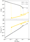 |
Fig. 7. Thermal solutions of the MAD numerical simulation for an XRB with MBH = 10 M⊙ at two different radii of r = 8 rg (solid lines) and r = 3 rg (dashed lines). The gray lines show the hot, optically thin branches, and the gold lines show the cold, optically thick branches. The inner radii can stay hot to higher ṁ than the outer radii. |
The most interesting feature of the MAD simulation of SBD24 is that it can have two stable thermal solutions at the high end of the ṁ range. For r = 8 rg, two solutions exist in the range 0.001 ≲ ṁ ≲ 0.1, while for r = 3 rg, two solutions exist in the range 0.04 ≲ ṁ ≲ 0.5. The inner disk stays hot to larger ṁ, and the disk cools from the outside in. For r = 8 rg, the optically thin solution exists up to ṁ ≲ 0.1 so that our optically thin strongly magnetized solution can survive to values of ṁ that are an order of magnitude higher than the one-temperature hot-flow solution of Esin et al. (1996). The optically thin MAD solution acts as a prolongation at high ṁ of the solution from Esin et al. (1996). Our MAD simulation also has an optically thick solution that exists down to ṁ ≳ 0.001 for r = 8 rg and ṁ ≳ 0.04 for r = 3 rg. It is interesting to note that the optically thick MAD solution does not exist at any radius at low accretion rates, in contrast to the SS73 solution, which is a valid solution down to ṁ as low as ≈10−14, at which point it becomes optically thin. This is because the surface density is much lower (by almost two orders of magnitude) in the MAD numerical solution than in the SS73 analytical solution.
We also show in Fig. 6 the comparison between the thermal solutions coming from the MAD numerical simulation of SBD24 and the two-temperature JED semi-analytical solution of Marcel et al. (2018a) with a sonic Mach number ms ≡ vr/cs = 0.5 and βz, mid = 20. The JED solution has two thermal solutions in the range 6×10⁻⁵ ≲ ṁ ≲ 2 × 10⁻², but cannot stay optically thin for ṁ ≳ 2 × 10⁻²⁶. Our MAD simulation has ms ≈ 0.8 and βz, mid ≈ 26 (see Fig. 1). Despite this difference of 37% in ms (translating into a difference in Σ), the two situations can be readily compared, and the two stable thermal branches are shifted. In the MAD thermal solutions, the two stable thermal branches are shifted to higher ṁ by a factor of ≈6 compared to the JED thermal solutions. We show in Sect. 5.1 that the reasons for this difference lie in another phenomenon.
4.2. Tentative hysteresis cycle
There is ample evidence that the outbursts of X-ray binaries are triggered in the outer disk (Lasota 2001). One promising mechanism for triggering the eruption is the ionization instability model (see Coriat et al. 2012 for observational evidence supporting this mechanism), in which the instability triggers an increase in the accretion rate in the outer parts of the disk, which then propagates inward and places the entire disk in a highly accreting state. This is the rise to outburst. As accretion proceeds, it depletes the disk until the ionization instability is triggered again where the density is too low. This is the return to quiescence (Dubus et al. 2001; Lasota 2001). In this framework, all the timescales involved in the X-ray binary hysteresis are then governed by the outer disk, and we can treat the inner disk as being in a quasi-steady state with constant ṁ.
Although the hysteresis is a global problem involving a range of radii, we explain our scenario using a local approach, placing ourselves at r = 8 rg, for simplicity. We showed in the previous section that given our assumption that hρ ∝ T1/2, the MAD solution of SBD24 has two thermal equilibria in the range 0.001 ≲ ṁ ≲ 0.1 at r = 8 rg. We now make the crude approximation that the radiative efficiency is the same for the two thermal solutions above ṁ ≳ 0.01 and is ≈0.2, a value close to what is generally found in MAD simulations (Avara et al. 2016; Dexter et al. 2021; Liska et al. 2022; Scepi et al. 2024). With this radiative efficiency, our two solutions have the potential of producing a thermal hysteresis in the range of luminosities 0.004 ≲ L ≲ 0.2. This is very reminiscent of the range in which spectral hysteresis is observed in X-ray binaries. The radiative efficiency might be lower in the hard state than in the soft state by as much as a factor of 5 (see Fig.6 of Marcel et al. 2018b). This would reduce the maximum luminosity of the hard state and increase the maximum luminosity of the soft state. However, other effects such as X-ray absorption along the line of sight should be taken into account for a detailed comparison with observations, and our assumption of a constant radiative efficiency is only a first step for this exploratory paper.
We showed in Sect. 3 that the hot, optically thin (cold, optically thick, respectively) MAD solution qualitatively has the right temperatures to produce a hard state (soft state7, respectively). Now, we can draw a sketch for a tentative spectral hysteresis cycle. We assumed that the inner disk stays MAD (i.e., stays highly magnetized) throughout the outburst, and we assumed a radiative efficiency of 0.2 for simplicity. The disk starts in quiescence, and ṁ starts increasing at the beginning of the outburst. It was shown by Dexter et al. (2021) that MADs can reproduce the properties of the hard state (power-law and cutoff evolution) from quiescence to L ≲ 10−3 LEdd. For L ≳ 10−3 LEdd, the disk starts to cool to temperatures close to 109 K (Dexter et al. 2021), at which point the magnetization increases even further (SBD24). This extremely magnetically dominated state can sustain a hot, optically thin solution, which can be seen as a magnetized extension of the hot one-temperature flow of Esin et al. (1996) (see Fig. 6), as was also found in the JED solutions of Petrucci et al. (2010), Marcel et al. (2018a). Consequently, the disk naturally transits from one optically thin solution to the next. The disk tracks the optically thin solution until the latter ceases to exist. In a MAD, this occurs at L ≈ 0.2 LEdd (at r = 8 rg), although the exact value would change if on-the-fly radiation were included in the simulation. At this point, the disk has to switch to the only available solution, which is the cold, optically thick one. This corresponds to the transition to the soft state at high luminosities. Similarly, as ṁ decreases back to quiescence, the disk stays in the cold, optically thick solution until this solution ceases to exist. In a MAD, this occurs for L ≲ 0.004 LEdd (at r = 8 rg), where the only available solution is the hot, optically thin one. Again, the exact value most likely changes when more realistic simulations of this very cold state are available. Nonetheless, the disappearance of the cold solution offers a physical mechanism for X-ray binaries to transit back from the soft state to the hard state at L ≈ 10−2 LEdd. Finally, the disk returns to quiescence and stays in the only available solution, the hot, optically thin one, and a new cycle begins.
In this scenario, we assumed that the disk keeps the same magnetization level during the entire outburst. This means that although the radial dependence of Bz is fixed, the absolute value of Bz needs to adjust to the evolving accretion rate. Magnetic rearrangements are expected to occur on a timescale that is at least as fast as the accretion timescale (Jacquemin-Ide et al. 2021), so that this is not an issue. In our scenario, however, we need to keep a strongly magnetized disk even at low hth/r, which has historically been known to be a potential issue (Lubow et al. 1994). However, every simulation of magnetized thin disks has shown so far (Avara et al. 2016; Liska et al. 2018, 2022; Zhu & Stone 2018; Mishra et al. 2020; Scepi et al. 2024) that thin disks are able to retain a strong magnetic field even for hth/r as low as 0.03. Still, the regime of h/r ≈ 10−3 that we reach in the soft state remains inaccessible to numerical simulations, and our hypothesis that thin disks can be highly magnetized throughout an entire outburst therefore remains to be confirmed with future numerical simulations.
We focused on the simplest features of the hysteresis cycle of XRBs. However, many XRBs show more complex behaviors, such as failed transitions to the soft state or different transition luminosities from the hard to the soft state in a given object. These complex behaviors are likely to involve the physics of the entire disk, for instance, how the outer disk feeds the inner disk with a magnetic field and impacts its magnetization. It is beyond the scope of this paper to explain these features. We focused here on the physics of the inner disk.
5. Discussion
5.1. Comparison to the literature
Very few simulations in the geometrically thin magnetized regime exist for comparison with this work. Nonetheless, our work agrees to some extent with the recent radiative GRMHD simulation of Liska et al. (2022), who showed that a thin disk at L = 0.3 LEdd naturally evolves to a temperature of 109 K when it is strongly magnetized. This hot solution is allowed because, as in the simulation of SBD24, the density is much lower than in standard theory. However, we find that our simulation should be one-temperature at a high accretion rate, in contrast to Liska et al. (2022). Moreover, we argue from our present analysis that there should be another solution that is optically thick at the same luminosity. This solution, however, would be hard to obtain from a radiative GRMHD simulation since it requires a start from a very cold disk. Numerical simulations are now restricted because of the resolution to aspect ratios of hth/r ≈ 0.03, while a temperature of 107 K corresponds to hth/r ≈ 10−3, which is lower by an order of magnitude than what is currently feasible.
We pointed out above the similarities between MAD numerical simulations and the JED semi-analytical solutions of Petrucci et al. (2008, 2010), Marcel et al. (2018a, b, 2019). In Fig. 6, we plot our thermal solutions for our MAD simulation over a two-temperature JED solution with similar properties, that is, a sonic Mach number of ms = 0.5 and a βz, mid = 20. The JED solution has two thermal solutions in the range 6 × 10⁻⁵ ≲ ṁ ≲ 2 × 10⁻², which is lower by roughly an order of magnitude than in our case. This difference can probably be attributed to two effects:
(1) The effective scale height of the disk in our MAD solution was set to 3hth (due to the additional support of magnetic pressure), while in the JED, it was set to hth. Because the surface densities between the JED and the MAD hot solutions are roughly similar (see Fig. 6), this means that our MAD solution is three times less dense than the JED solution for a given accretion rate8.
(2) An additional source of energy comes from the innermost part of the disk in the MAD solution compared to the JED solution. To see this additional energy input, we refer to Appendix A, where we analyze the energy balance of our MAD simulation in detail. Briefly, we find that in our MAD solution, there is roughly twice the local binding energy that is available at large radii because magnetic stresses redistribute energy outward from the innermost radii (including the plunging region). In contrast, in the JED framework, it is assumed that only the local binding energy is available at each radius (Marcel et al. 2018a). This comes from the neglected GR effects and the related assumption of a Newtonian Keplerian rotation law. These assumptions forbids an innermost plunging region where radially oriented magnetic field lines are able to efficiently transfer angular momentum in the radial direction.
5.2. A dark jet?
A prominent feature of the hard-to-soft state transition is the disappearance of the radio emission, which is associated with a compact jet (Mirabel & Rodriguez 1994; Fender et al. 1999; Tetarenko et al. 2017). The upper limits on the radio flux in 4U 1957+11 show that the radio emission from the jet is reduced by at least 2.5 orders of magnitudes when it enters the soft state (Russell et al. 2011). Many scenarios therefore advocate for a change in the magnetization as the driver of the hard-to-soft state transition (Ferreira et al. 2006; Igumenshchev 2009; Begelman & Armitage 2014). We argue that if the XRB hysteresis is driven by a thermal hysteresis, a high magnetization must be present throughout the XRB outburst to explain the state transition luminosities. Hence, we would expect that a powerful Blandford-Znakek jet (Blandford & Znajek 1977) is present during the entire outburst since it is an unavoidable outcome of every MAD simulation. However, we argue that it is not clear that this jet would be visible throughout the outburst for two reasons. First, SBD24 reported that the efficiency of the BZ jet evolves as hth/r, so that the radio emission could be expected to decrease by a factor of as much as 100 when going from the hard state to the soft state. Avara et al. (2016) suggested an even steeper dependence of the jet efficiency of (hth/r)2. This is marginally enough to explain the quenching of the jet. The second point is that the power of the BZ jet is related in a no-trivial way to the radio emission that is observed. The particles need to be accelerated somehow, and there is no consensus regarding the origin of the particle acceleration in jets. The internal shock model of Malzac (2013) suggested that particles are accelerated inside shocks due to to the differential jet velocity. One prediction of this internal shock model is the presence of a dark weakly dissipative jet in the soft state (Drappeau et al. 2017; Péault et al. 2019), which would fit our scenario well9. Other models invoking particle acceleration in the sheath of the jet at the interface with the wind or accretion flow (Sironi et al. 2021) could produce a weakly dissipative jet in the soft state. Because the disk is much thinner in the soft state, it would indeed be natural to expect the interaction between the jet sheath and the wind or accretion flow to be much weaker in the soft state than in the hard state. Recent improvements in radio sensitivity with the Square Kilometre Array telescope (SKA) might allow us to revisit the lower radio-detection limits and test again for the presence of a weak jet in the soft state of XRBs.
5.3. Application to AGN
It is often argued that AGN are scaled-up versions of XRBs, so that the population of AGN should imprint the properties of the XRB hysteresis (Körding et al. 2008; Ruan et al. 2019; Fernández-Ontiveros & Muñoz-Darias 2021; Hagen et al. 2024). To test this hypothesis, we applied our post-processing procedure to determine the thermal equilibrium curves of an AGN around a BH of MBH = 108 M⊙. Figure 8 shows the comparison of the thermal hysteresis drawn by an AGN (solid line) compared to an XRB (dashed line). The AGN case has a thermal hysteresis over a much wider range of ṁ from 3 × 10⁻⁸ ≲ ṁ ≲ 0.1, compared to 10−3 ≲ ṁ ≲ 0.1 for the XRB case. While the hot, optically thin branch has its highest ṁ in equilibrium at ≈0.1 in both the AGN and XRB cases, the cold, optically thick branch has its lowest ṁ in equilibrium at ≈3 × 10⁻⁸ in the AGN case, that is, much lower than the ṁ ≈10−3 for the XRB case. This difference arises because on the cold, optically thick branch, the temperature of an AGN is much lower than that of an XRB. Since the Rosseland opacity depends so drastically on temperature, this means that the density for an AGN has to decrease by a very large amount compared to an XRB for the disk to become optically thin on the cold branch.
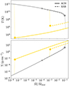 |
Fig. 8. Comparison of the thermal solutions for the MAD numerical simulation at r = 8 rg in an AGN with MBH = 108 M⊙ (solid lines) and in an XRB with MBH = 10 M⊙ (dashed lines). The gray and gold lines show the hot and cold branches, respectively. The hysteresis cycle for AGN extends over a much wider range of ṁ, so that low-luminosity AGN with ṁ as low as 10−7 are expected to be found in a disk-like spectral state. |
In our thermal hysteresis scenario, we would therefore not expect AGN and XRB to have the same hysteresis cycle. The properties of an individual object in the hard state are expected to be similar in an AGN and an XRB, for example, the anticorrelation between the X-ray hardness and the luminosity above 10−2 LEdd. However, in contrast to XRBs, we expect to find that low-luminosity AGN with ṁ ≳ 10−7 are divided quite evenly between objects with a hard-state and a soft-state spectrum. The exact ratio of hard- to soft-state objects at a given luminosity depends on the ratio of the time spent during the rise to outburst compared to the time spent during the decay to quiescence. This ratio in turn depends on the mechanism that drives the AGN eruptions. The ionization instability model, which was successfully applied to XRBs, fails to explain the AGN population properties and does not produce outbursts similar to the XRB case (Hameury et al. 2009). A mechanism involving gravitational instability in the outer disk might also be at work, and so it is unclear what the secular outburst of an AGN should look like. Moreover, the few changing-look AGN that are observed to change spectral states evolve on timescales that are much shorter than a scale-up of the XRB timescales. This makes it hard for us to give a precise number for the expected fraction of low-luminosity AGN in a soft disk-like state. Nonetheless, this fraction is expected to be higher than in XRBs, and we do not expect to retrieve an observed lack of soft-state AGN below 10−2 LEdd, as is usually expected in analogy to XRBs. While recent observational surveys by Fernández-Ontiveros & Muñoz-Darias (2021) and Hagen et al. (2024) have suggested that all AGN do transit to a hard state below 10−2 Eddington, we note that a recent X-ray sky-survey by eROSITA found a lack of soft X-ray emitting AGN compared to what was expected from models based on the XRB analogy (Arcodia et al. 2024). Clearly, this crucial point deserves a more detailed study on the theoretical and observational fronts.
6. Conclusions
We have studied the thermal properties of wind-driven accretion disks that are magnetically dominated (βz, mid < 100). They are recognized as MADs in GRMHD simulations or as JEDs in analytical studies. By including radiative cooling in post-processing in a simulation from SBD24, we solved for all the equilibrium temperatures of the disk at different accretion rates during an XRB outburst.
We found that a MAD can maintain a hot inner disk (with temperatures ≳108 − 9 K) up to luminosities as high as 0.2 LEdd (for an accretion efficiency of ≈0.2), which might explain the high-luminosity hard state in XRBs. This hot inner disk is not homogeneous, with cold patches of dense gas in the midplane. The hot inner disk cools from the outside in as the luminosity increases, yielding a truncation radius (i.e., a transition radius between a hot, optically thin inner disk and a cold, optically thick outer disk) that moves inward with increasing luminosity.
By assuming simple scalings for the disk scale height and accretion speed with temperature, we find that magnetically arrested disks have two thermal equilibrium solutions in the regime of 0.001 ≲ ṁ ≲ 0.1 at r = 8 rg and 0.04 ≲ ṁ ≲ 0.5 at r = 3 rg. This provides the means for a thermal hysteresis in XRBs without invoking a strong ADAF-principle, as is often done. Starting from the quiescent state, the disk stays in the hard state until no hot solution is possible any longer. This occurs around 0.2 LEdd at r = 8 rg, where the disk reaches the only available solution, the cold branch. In quiescence, the disk then stays in the cold solution until it ceases to exist. At 8 rg, this occurs at luminosities of ≈0.002 LEdd. Within our assumptions, our transition luminosities between the cold and hot solutions match the transitions observed in the hysteresis of XRBs reasonably well. We found that our transition luminosities are six times higher than in the case of the Newtonian JED semi-analytical solution of Marcel et al. (2018a) because of the effect of magnetic pressure and additional energy transport, mediated by magnetic stresses, from the innermost part of the disk below the ISCO.
Finally, we emphasize that in our case, the spectral hysteresis is purely thermal and the disk is always strongly magnetized. This means that we expect a jet, although possibly weakly dissipative, to be present even in the soft state. We also naively extrapolated our analysis to the case of AGN and found that the hysteresis would occur over a much wider range of accretion rate, that is, for 10−7 ≲ ṁ ≲ 2 × 10⁻¹. This means that under the hypothesis that the structure of the inner disk of an AGN is the same as that of an XRB, we expect a significantly larger fraction of low-luminosity AGN to be in a soft state compared to the XRB case.
Although note that the high X-ray polarization degree seen in Cyg X-1 seems to point towards a moderately relativistic outflowing corona (Poutanen et al. 2023; Dexter & Begelman 2024).
See SBD24 for the definition of the heating rate.
Note that the importance of external Compton also depends a lot on the geometry of the outer optically thick disk that irradiates the inner optically thin corona. For a very flared outer disk, external Compton could become important (see Marcel et al. 2018b).
Our computation of the opacities can only be an approximation without a proper radiative transfer that follows the path of individual photons.
Note that our solutions being one-temperature, the temperature of the optically thin solution for ṁ ≲ 0.01 is likely to be underestimated. However, since our focus is mostly on the high luminosity regime this approximation is of little consequence here.
To fit the X-ray spectrum of XRBs at high luminosity, such as GX 339-4 (Marcel et al. 2019) or MAXI J1820+070 (Marino et al. 2021), a larger ms = 1.5 is used for the JED semi-analytical solution. However, note that those solutions at high ms do not posses a cold, optically thick thermal solution.
The relatively low densities and strong dissipation away from the midplane in our cold, optically thick solution might produce large color corrections. This might make it challenging to reproduce the spectrum of XRBs with very soft states, such as LMC-X3, where spin measurements through continuum fitting with moderate color corrections already give a low spin value (Davis et al. 2006; Yilmaz et al. 2023). However, a large color correction might help to explain the apparent sizes of AGN (Hall et al. 2018).
A turbulent magnetic pressure in JED solutions was recently included by Zimniak et al. (2024).
In the original idea of the internal shock model, the fluctuations in velocity in a Blandford-Payne-type jet cause the shocks. These fluctuations themselves are driven by the fluctuations in the accretion rate in the disk. Here, we implicitly assumed that the relation between the jet and the accretion flow is the same, regardless of whether the jet is driven by a Blandford-Znajek or Blandford-Payne mechanism.
We add the continuity equation to remove the rest-mass energy contribution (see Sądowski 2016).
tbeg and tend are defined in SBD24
Note that radial derivatives introduce a lot of noise in the procedure.
Acknowledgments
We thank the referee for their constructive report that improved siginificantly the clarity of our paper. NS thanks Eliot Quataert for fruitful discussions on an early version of the paper and for suggesting that we extend our scenario to AGN. NS acknowledges partial financial support from the European Research Council (ERC) under the European Union Horizon 2020 research and innovation programme (Grant agreement No. 815559 (MHDiscs)) and the UK’s Science and Technology Facilities Council [ST/M001326/1]. We also acknowledge financial support from NASA Astrophysics Theory Program grants NNX16AI40G, NNX17AK55G, 80NSSC20K0527, 80NSSC22K0826 and an Alfred P. Sloan Research Fellowship (JD). GM acknowledges financial support from the Polish National Science Center grant 2023/48/Q/ST9/00138.
References
- Agol, E., & Krolik, J. H. 2000, ApJ, 528, 161 [NASA ADS] [CrossRef] [Google Scholar]
- Alabarta, K., Altamirano, D., Méndez, M., et al. 2021, MNRAS, 507, 5507 [NASA ADS] [CrossRef] [Google Scholar]
- Arcodia, R., Merloni, A., Comparat, J., et al. 2024, A&A, 681, A97 [NASA ADS] [CrossRef] [EDP Sciences] [Google Scholar]
- Artemova, I. V., Bisnovatyi-Kogan, G. S., Bjoernsson, G., & Novikov, I. D. 1996, ApJ, 456, 119 [NASA ADS] [CrossRef] [Google Scholar]
- Avara, M. J., McKinney, J. C., & Reynolds, C. S. 2016, MNRAS, 462, 636 [NASA ADS] [CrossRef] [Google Scholar]
- Bambic, C. J., Quataert, E., Kunz, M. W., & Jiang, Y.-F. 2024, MNRAS, 530, 1812 [CrossRef] [Google Scholar]
- Begelman, M. C., & Armitage, P. J. 2014, ApJ, 782, L18 [NASA ADS] [CrossRef] [Google Scholar]
- Blandford, R. D., & Payne, D. G. 1982, MNRAS, 199, 883 [CrossRef] [Google Scholar]
- Blandford, R. D., & Znajek, R. L. 1977, MNRAS, 179, 433 [NASA ADS] [CrossRef] [Google Scholar]
- Cangemi, F., Rodriguez, J., Belloni, T., et al. 2023, A&A, 669, A65 [NASA ADS] [CrossRef] [EDP Sciences] [Google Scholar]
- Cao, X. 2016, ApJ, 817, 71 [NASA ADS] [CrossRef] [Google Scholar]
- Corbel, S., Dubus, G., Tomsick, J. A., et al. 2012, MNRAS, 421, 2947 [CrossRef] [Google Scholar]
- Coriat, M., Fender, R. P., & Dubus, G. 2012, MNRAS, 424, 1991 [NASA ADS] [CrossRef] [Google Scholar]
- Dauser, T., Garcia, J., Wilms, J., et al. 2013, MNRAS, 430, 1694 [Google Scholar]
- Davis, S. W., Done, C., & Blaes, O. M. 2006, ApJ, 647, 525 [NASA ADS] [CrossRef] [Google Scholar]
- Dexter, J., & Begelman, M. C. 2024, MNRAS, 528, L157 [Google Scholar]
- Dexter, J., Scepi, N., & Begelman, M. C. 2021, ApJ, 919, L20 [NASA ADS] [CrossRef] [Google Scholar]
- Done, C., Gierliński, M., & Kubota, A. 2007, A&ARv., 15, 1 [NASA ADS] [CrossRef] [Google Scholar]
- Drappeau, S., Malzac, J., Coriat, M., et al. 2017, MNRAS, 466, 4272 [NASA ADS] [Google Scholar]
- Dubus, G., Hameury, J. M., & Lasota, J. P. 2001, A&A, 373, 251 [NASA ADS] [CrossRef] [EDP Sciences] [Google Scholar]
- Dunn, R., Fender, R., Körding, E., Belloni, T., & Cabanac, C. 2010, MNRAS, 403, 61 [NASA ADS] [CrossRef] [Google Scholar]
- Esin, A. A., Narayan, R., Ostriker, E., & Yi, I. 1996, ApJ, 465, 312 [Google Scholar]
- Esin, A. A., McClintock, J. E., & Narayan, R. 1997, ApJ, 489, 865 [NASA ADS] [CrossRef] [Google Scholar]
- Fender, R., Corbel, S., Tzioumis, T., et al. 1999, ApJ, 519, L165 [NASA ADS] [CrossRef] [Google Scholar]
- Fender, R. P., Belloni, T. M., & Gallo, E. 2004, MNRAS, 355, 1105 [NASA ADS] [CrossRef] [Google Scholar]
- Fender, R. P., Homan, J., & Belloni, T. M. 2009, MNRAS, 396, 1370 [NASA ADS] [CrossRef] [Google Scholar]
- Fernández-Ontiveros, J. A., & Muñoz-Darias, T. 2021, MNRAS, 504, 5726 [CrossRef] [Google Scholar]
- Ferreira, J. 1997, A&A, 319, 340 [Google Scholar]
- Ferreira, J., & Pelletier, G. 1993, A&A, 276, 625 [NASA ADS] [Google Scholar]
- Ferreira, J., & Pelletier, G. 1995, A&A, 295, 807 [NASA ADS] [Google Scholar]
- Ferreira, J., Petrucci, P.-O., Henri, G., Saugé, L., & Pelletier, G. 2006, A&A, 447, 813 [NASA ADS] [CrossRef] [EDP Sciences] [Google Scholar]
- Fishbone, L. G., & Moncrief, V. 1976, ApJ, 207, 962 [NASA ADS] [CrossRef] [Google Scholar]
- Grošelj, D., Hakobyan, H., Beloborodov, A. M., Sironi, L., & Philippov, A. 2024, Phys. Rev. Lett., 132, 085202 [CrossRef] [Google Scholar]
- Grove, J. E., Johnson, W. N., Kroeger, R. A., et al. 1998, ApJ, 500, 899 [NASA ADS] [CrossRef] [Google Scholar]
- Haardt, F., Maraschi, L., & Ghisellini, G. 1994, ApJ, 432, L95 [NASA ADS] [CrossRef] [Google Scholar]
- Hagen, S., Done, C., Silverman, J. D., et al. 2024, MNRAS, 534, 2803 [NASA ADS] [CrossRef] [Google Scholar]
- Hall, P. B., Sarrouh, G. T., & Horne, K. 2018, ApJ, 854, 93 [Google Scholar]
- Hameury, J.-M., Viallet, M., & Lasota, J.-P. 2009, A&A, 496, 413 [NASA ADS] [CrossRef] [EDP Sciences] [Google Scholar]
- Hankla, A. M., Scepi, N., & Dexter, J. 2022, MNRAS, 515, 775 [NASA ADS] [CrossRef] [Google Scholar]
- Henri, G., & Petrucci, P. O. 1997, A&A, 326, 87 [NASA ADS] [Google Scholar]
- Igumenshchev, I. V. 2008, ApJ, 677, 317 [NASA ADS] [CrossRef] [Google Scholar]
- Igumenshchev, I. V. 2009, ApJ, 702, L72 [NASA ADS] [CrossRef] [Google Scholar]
- Jacquemin-Ide, J., Lesur, G., & Ferreira, J. 2021, A&A, 647, A192 [EDP Sciences] [Google Scholar]
- Jourdain, E., Roques, J. P., Chauvin, M., & Clark, D. J. 2012, ApJ, 761, 27 [NASA ADS] [CrossRef] [Google Scholar]
- Kinch, B. E., Schnittman, J. D., Noble, S. C., Kallman, T. R., & Krolik, J. H. 2021, ApJ, 922, 270 [CrossRef] [Google Scholar]
- Körding, E., Rupen, M., Knigge, C., et al. 2008, Science, 320, 1318 [CrossRef] [Google Scholar]
- Krawczynski, H., Muleri, F., Dovčiak, M., et al. 2022, Science, 378, 650 [NASA ADS] [CrossRef] [Google Scholar]
- Lasota, J.-P. 2001, New Astron. Rev., 45, 449 [Google Scholar]
- Laurent, P., Rodriguez, J., Wilms, J., et al. 2011, Science, 332, 438 [Google Scholar]
- Liska, M., Hesp, C., Tchekhovskoy, A., et al. 2018, MNRAS, 474, L81 [Google Scholar]
- Liska, M. T. P., Musoke, G., Tchekhovskoy, A., Porth, O., & Beloborodov, A. M. 2022, ApJ, 935, L1 [NASA ADS] [CrossRef] [Google Scholar]
- Lubow, S. H., Papaloizou, J. C. B., & Pringle, J. E. 1994, MNRAS, 267, 235 [NASA ADS] [Google Scholar]
- Maccarone, T. J. 2003, A&A, 409, 697 [NASA ADS] [CrossRef] [EDP Sciences] [Google Scholar]
- Mahadevan, R., & Quataert, E. 1997, ApJ, 490, 605 [Google Scholar]
- Malzac, J. 2013, MNRAS, 429, L20 [NASA ADS] [CrossRef] [Google Scholar]
- Manikantan, V., Kaaz, N., Jacquemin-Ide, J., et al. 2024, ApJ, 965, 175 [NASA ADS] [CrossRef] [Google Scholar]
- Marcel, G., Ferreira, J., Petrucci, P. O., et al. 2018a, A&A, 615, A57 [NASA ADS] [CrossRef] [EDP Sciences] [Google Scholar]
- Marcel, G., Ferreira, J., Petrucci, P. O., et al. 2018b, A&A, 617, A46 [NASA ADS] [CrossRef] [EDP Sciences] [Google Scholar]
- Marcel, G., Ferreira, J., Clavel, M., et al. 2019, A&A, 626, A115 [NASA ADS] [CrossRef] [EDP Sciences] [Google Scholar]
- Marino, A., Barnier, S., Petrucci, P. O., et al. 2021, A&A, 656, A63 [NASA ADS] [CrossRef] [EDP Sciences] [Google Scholar]
- Markoff, S., Nowak, M. A., & Wilms, J. 2005, ApJ, 635, 1203 [NASA ADS] [CrossRef] [Google Scholar]
- Martocchia, A., & Matt, G. 1996, MNRAS, 282, L53 [NASA ADS] [CrossRef] [Google Scholar]
- Matt, G., Perola, G., & Piro, L. 1991, A&A, 247, 25 [Google Scholar]
- McKinney, J. C., Tchekhovskoy, A., & Blandford, R. D. 2012, MNRAS, 423, 3083 [Google Scholar]
- Meyer, F., & Meyer-Hofmeister, E. 1994, A&A, 288, 175 [NASA ADS] [Google Scholar]
- Mirabel, I., & Rodriguez, L. 1994, Nature, 371, 46 [NASA ADS] [CrossRef] [Google Scholar]
- Mishra, B., Begelman, M. C., Armitage, P. J., & Simon, J. B. 2020, MNRAS, 492, 1855 [NASA ADS] [CrossRef] [Google Scholar]
- Narayan, R. 1996, ApJ, 462, 136 [Google Scholar]
- Noble, S. C., Krolik, J. H., & Hawley, J. F. 2009, ApJ, 692, 411 [NASA ADS] [CrossRef] [Google Scholar]
- Oda, H., Machida, M., Nakamura, K. E., Matsumoto, R., & Narayan, R. 2012, PASJ, 64, 15 [NASA ADS] [CrossRef] [Google Scholar]
- Péault, M., Malzac, J., Coriat, M., et al. 2019, MNRAS, 482, 2447 [CrossRef] [Google Scholar]
- Petrucci, P.-O., Ferreira, J., Henri, G., & Pelletier, G. 2008, MNRAS, 385, L88 [NASA ADS] [CrossRef] [Google Scholar]
- Petrucci, P.-O., Ferreira, J., Henri, G., Malzac, J., & Foellmi, C. 2010, A&A, 522, A38 [NASA ADS] [CrossRef] [EDP Sciences] [Google Scholar]
- Poutanen, J., & Veledina, A. 2014, Space Sci. Rev., 183, 61 [CrossRef] [Google Scholar]
- Poutanen, J., Veledina, A., & Beloborodov, A. M. 2023, ApJ, 949, L10 [NASA ADS] [CrossRef] [Google Scholar]
- Remillard, R. A., & McClintock, J. E. 2006, ARA&A, 44, 49 [Google Scholar]
- Ruan, J. J., Anderson, S. F., Eracleous, M., et al. 2019, ApJ, 883, 76 [NASA ADS] [CrossRef] [Google Scholar]
- Russell, D., Miller-Jones, J., Maccarone, T., et al. 2011, ApJ, 739, L19 [NASA ADS] [CrossRef] [Google Scholar]
- Sądowski, A. 2016, MNRAS, 459, 4397 [CrossRef] [Google Scholar]
- Scepi, N., Begelman, M. C., & Dexter, J. 2024, MNRAS, 527, 1424 [Google Scholar]
- Schnittman, J. D., Krolik, J. H., & Noble, S. C. 2013, ApJ, 769, 156 [NASA ADS] [CrossRef] [Google Scholar]
- Shakura, N. I., & Sunyaev, R. A. 1973, A&A, 24, 337 [NASA ADS] [Google Scholar]
- Shaw, A., Gandhi, P., Altamirano, D., et al. 2016, MNRAS, 458, 1636 [NASA ADS] [CrossRef] [Google Scholar]
- Sironi, L., Rowan, M. E., & Narayan, R. 2021, ApJ, 907, L44 [CrossRef] [Google Scholar]
- Spruit, H. C., & Deufel, B. 2002, A&A, 387, 918 [NASA ADS] [CrossRef] [EDP Sciences] [Google Scholar]
- Sridhar, N., Sironi, L., & Beloborodov, A. M. 2021, MNRAS, 507, 5625 [NASA ADS] [CrossRef] [Google Scholar]
- Stone, J. M., Tomida, K., White, C. J., & Felker, K. G. 2020, Am. Astron. Soc., 249, 4 [Google Scholar]
- Sunyaev, R., & Titarchuk, L. 1980, A&A, 86, 121 [NASA ADS] [Google Scholar]
- Tetarenko, B. E., Sivakoff, G. R., Heinke, C. O., & Gladstone, J. C. 2016, ApJS, 222, 15 [Google Scholar]
- Tetarenko, A. J., Sivakoff, G. R., Miller-Jones, J. C., et al. 2017, MNRAS, 469, 3141 [NASA ADS] [CrossRef] [Google Scholar]
- White, C. J., Stone, J. M., & Gammie, C. F. 2016, ApJS, 225, 22 [NASA ADS] [CrossRef] [Google Scholar]
- Yilmaz, A., Svoboda, J., Grinberg, V., et al. 2023, MNRAS, 525, 1288 [CrossRef] [Google Scholar]
- Yuan, F., & Narayan, R. 2014, ARA&A, 52, 529 [NASA ADS] [CrossRef] [Google Scholar]
- Zdziarski, A. A., Lubiński, P., & Sikora, M. 2012, MNRAS, 423, 663 [NASA ADS] [CrossRef] [Google Scholar]
- Zhu, Z., & Stone, J. M. 2018, ApJ, 857, 34 [Google Scholar]
- Zimniak, N., Ferreira, J., & Jacquemin-Ide, J. 2024, A&A, 692, A99 [NASA ADS] [CrossRef] [EDP Sciences] [Google Scholar]
Appendix A: Energy balance in a MAD simulation
We start by recalling that the continuity equation and the conservation of energy in GRMHD read as
 (A.1)
(A.1)
 (A.2)
(A.2)
where the stress-energy tensor is
 (A.3)
(A.3)
and ℱμ represents an optically thin cooling source term that is defined as in Noble et al. (2009). Additionally, pgas is the gas pressure, ug = pgas/(γad − 1) is the internal energy of the gas in the comoving frame, γad = 5/3 is the adiabatic index and bμ is the fluid frame 4-magnetic field.
We then define a surface delimiting the boundary between the disk and the wind. For simplicity, we define this boundary at a fixed θ to have only fluxes along θ in the wind contribution and fluxes along r in the disk contribution. We define this boundary at θ± = π/2 ± π/8. We have checked that our choice of the disk surface is close to the surface where the angular momentum flux, Tϕr, changes sign (Ferreira & Pelletier 1995; Manikantan et al. 2024). We then integrate the sum of Eq. A.1 and Eq. A.2 10 over the volume [tbeg, tend]×[θ+, θ−]×[0, 2π] in the t, θ, ϕ11 directions and we assume steady-state conditions to define qtot, the total energy loss in the disk,
![Mathematical equation: $$ \begin{aligned} q_{\rm tot}\equiv \int ^{\theta ^+}_{\theta ^-} \partial _r(\sqrt{-g} \langle T^{r}_{t} \rangle )d\theta + \big [ \sqrt{-g} \langle T^{\theta }_{t} \rangle \big ]^{\theta ^+}_{\theta ^-} + \int ^{\theta ^+}_{\theta ^-} \sqrt{-g}\langle \mathcal{F} _t \rangle d\theta = 0, \end{aligned} $$](/articles/aa/full_html/2024/12/aa51568-24/aa51568-24-eq21.gif) (A.4)
(A.4)
where ⟨⟩ means an azimuthal and time average. We see that by construction, qtot should be equal to 0. This can be seen to be approximately true 12 on Fig. A.1 except near the horizon where the heavy use of ceilings on the magnetic field breaks energy conservation.
To gain physical insight, we decompose qtot into five type of energy losses that reduce to well-known quantities in a Newtonian framework. With this decomposition, we have
 (A.5)
(A.5)
with
 (A.6)
(A.6)
 (A.7)
(A.7)
 (A.8)
(A.8)
![Mathematical equation: $$ \begin{aligned} q_{\rm Stress}&= \int _{\theta } \partial _r(\sqrt{-g}\langle \delta ([\rho +\gamma _{\rm ad}u_g] u^r) \delta u_t + b^2 u^ru_t -b^rb_t \rangle ) d\theta , \end{aligned} $$](/articles/aa/full_html/2024/12/aa51568-24/aa51568-24-eq26.gif) (A.9)
(A.9)
![Mathematical equation: $$ \begin{aligned} q_{\rm Wind}&= \big [ \sqrt{-g}\langle (\rho +\gamma _{\rm ad}u_g+b^2) u^\theta u_t -b^\theta b_t \rangle \big ]^{\theta _{\rm +}}_{\theta _{\rm -}}. \end{aligned} $$](/articles/aa/full_html/2024/12/aa51568-24/aa51568-24-eq27.gif) (A.10)
(A.10)
Here qRad is the radiative energy loss, qBind is the binding energy loss, qAdv is the disk internal energy advection energy loss, qStress is the energy loss due to stresses through the disk and qWind is the energy loss due to the wind. Note that to define qBind, qAdv and qStress we divided the ⟨(ρ + γadug)urut⟩ into a laminar component ⟨(ρ + γadug)ur⟩⟨ut⟩ (going into qBind and qAdv) and a turbulent component ⟨δ([ρ + γadug]ur)δut⟩≡⟨(ρ + γadug)urut⟩−⟨(ρ + γadug)ur⟩⟨ut⟩ (going into qStress).
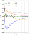 |
Fig. A.1. Balance of energy loss or gain in the disk as a function of radius. The blue, green, red, grey and gold lines show respectively qBind (the binding energy gain), qAdv (the disk internal energy advected energy), qRad (the radiative energy loss), LWind (energy loss due to the wind) and qStress (energy loss or gain due to stresses in the disk). qStress changes sign around 4.5 rg meaning that energy is redistributed from the inner region to the outer regions of the disk by magnetic stresses. |
We plot on Fig. A.1 these five contributions. Note that a positive (negative) energy loss means that the disk effectively loses (gains) energy. For example, qRad, qAdv and qWind are positive, meaning that radiation, advection and the wind remove energy from the disk. In fact, advection is almost negligible here but the wind takes a large part of the energy compared to radiation. On the other hand, qBind is negative meaning that binding energy is deposited in the disk. Now, qStress changes sign around 4.5 rg going from positive to negative. This means that energy is redistributed from the inner region to the outer regions of the disk by magnetic stresses. This is similar to what happens in a standard model using a zero-torque boundary condition at the horizon of the black hole (but not at the ISCO as usually assumed). We find that this redistribution of energy can induce a local energy gain that can be as much as 3.5 times the local binding energy gain at r = 10 rg.
To be more quantitative, we look at the difference of the luminosities between 7.5 rg and 8.5 rg to see how much energy is deposited or taken away at r = 8 rg (the radius at which Fig. 6 is made). We write ΔEX = ∫7.5 rg8.5 rgqXdr. As such, we can rewrite Eq. A.5 in a form close to Eq. 10 of Petrucci et al. (2010),
 (A.11)
where −ΔEStress represents an additional source of energy, on top of the local binding energy, compared to the Eq. 10 of Petrucci et al. (2010).
We find that ΔERad ≈ 0.33, ΔEBind ≈ −0.48, ΔEAdv ≈ 0.005, ΔEStress ≈ −0.77 and ΔEWind ≈ 0.90. Again, this means that roughly 2.5 times the equivalent of the binding energy is locally available at each radii. Out of this local energy roughly three quarters is taken out by the wind while only one quarter is locally radiated away.
It is intriguing that qStress is not zero at the ISCO as this means that magnetic stresses could potentially tap into the rotational energy of the black hole inside the ergosphere. To check this idea, we have run a preliminary thin (hth/r = 0.03 as in SBD24) MAD simulation with zero spin. We find that qStress is similar in the cases with zero and high spin, disfavoring the rotational energy of the black hole as a source of energy here. Clearly, this point deserves more work and will be the subject of a separate paper (Scepi et al. in preparation), in which we will present the details of a simulation with zero spin.
Appendix B: Decomposition of the cooling mechanisms
Figures B.1 and B.2 respectively show the dominant cooling mechanisms in each cell of the grid in a poloidal cut and a midplane cut of the disk. The snapshots are the same as used in Fig. 3 and Fig. 4 to allow comparisons with the temperature maps. At low accretion rates, we see that the disk is cooling entirely through optically thin processes (synchrotron self-Compton (SSC) and bremsstrahlung self-Compton (BSC)). The inner parts of the disk are cooling mostly through SSC whereas the outer parts are cooling mostly through BSC. This is because the magnetic field goes as r−1.5 whereas the density goes as r−1. Because of their low density, the upper layers of the disk are also dominated by SSC emission. As the accretion rate increases and the density increases, we see that BSC starts to gradually take over SSC in the inner disk. We also see that the densest part of the disk start to cool through optically thick black-body emission to form clumps of cold materials (as can be seen in Fig. 3 and Fig. 4.)
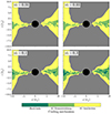 |
Fig. B.1. Poloidal cut showing the dominant cooling mechanism in each cell for four different ṁ. The grey region shows the jet region (defined as the region where σ > 1) that is excluded from our analysis. The snapshot used is the same as in Fig. 4 to allow comparison of the two Figures. |
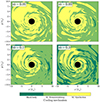 |
Fig. B.2. Midplane cut showing the dominant cooling mechanism in each cell for four different ṁ. The snapshot used is the same as in Fig. 3 to allow comparison of the two Figures. |
All Figures
|
Fig. 1. Radial profiles of the geometrical density scale height (solid gold line), the βz, mid in the midplane (solid blue line) and the density-weighted radial three-vector velocity normalized by the sound speed (dashed gray line). The density scale height and the radial speed exceed expectations from standard theory. |
| In the text | |
|
Fig. 2. Right panel: Time- and ϕ-averaged log of the density in the simulation of SBD24, normalized by the density in the midplane that would be obtained from the SS73 model with the same accretion rate, with α = 1 and hth/r = 0.03. The black lines show three contours of the color map. The gray lines show the surfaces of z/r = ±0.03. Left panel: Time- and ϕ-averaged cumulative heating rate, i.e., the ratio of the heating rate latitudinally integrated up to θ to the heating rate latitudinally integrated up to ∞. The black lines show three contours of the cumulative heating rate. |
| In the text | |
|
Fig. 3. Poloidal cuts of the post-processed temperature for four different accretion rates. The jet region (defined as the region where σ > 1) is excluded from our analysis. |
| In the text | |
|
Fig. 4. Midplane cut of the post-processed temperature for four different accretion rates. The temperature is inhomogeneous, but even at high accretion rates, patches of hot gas can survive. |
| In the text | |
|
Fig. 5. Poloidal cut of the yC Compton parameter and the ratio of the electron-proton collision time to the advection time. |
| In the text | |
|
Fig. 6. Thermal solutions of the MAD numerical simulation at r = 8 rg for an XRB with MBH = 10 M⊙. In both panels, the gray line shows the hot, optically thin branch that extends up to ṁ ≈ 10−1, while the gold line shows the cold, optically thick branch that only extends down to ṁ ≈ 10−3. The black lines show reference solutions for comparison with the dash-dotted, dotted, and dashed lines, which show the solutions for a standard Shakura-Sunyaev disk, a one-temperature ADAF analytical solution, and a two-temperature JED semi-analytical solution, respectively. The uniqueness of our MAD thermal solutions is that they have two stable thermal branches within the range 10−3 ≲ ṁ ≲ 10−1. |
| In the text | |
|
Fig. 7. Thermal solutions of the MAD numerical simulation for an XRB with MBH = 10 M⊙ at two different radii of r = 8 rg (solid lines) and r = 3 rg (dashed lines). The gray lines show the hot, optically thin branches, and the gold lines show the cold, optically thick branches. The inner radii can stay hot to higher ṁ than the outer radii. |
| In the text | |
|
Fig. 8. Comparison of the thermal solutions for the MAD numerical simulation at r = 8 rg in an AGN with MBH = 108 M⊙ (solid lines) and in an XRB with MBH = 10 M⊙ (dashed lines). The gray and gold lines show the hot and cold branches, respectively. The hysteresis cycle for AGN extends over a much wider range of ṁ, so that low-luminosity AGN with ṁ as low as 10−7 are expected to be found in a disk-like spectral state. |
| In the text | |
|
Fig. A.1. Balance of energy loss or gain in the disk as a function of radius. The blue, green, red, grey and gold lines show respectively qBind (the binding energy gain), qAdv (the disk internal energy advected energy), qRad (the radiative energy loss), LWind (energy loss due to the wind) and qStress (energy loss or gain due to stresses in the disk). qStress changes sign around 4.5 rg meaning that energy is redistributed from the inner region to the outer regions of the disk by magnetic stresses. |
| In the text | |
|
Fig. B.1. Poloidal cut showing the dominant cooling mechanism in each cell for four different ṁ. The grey region shows the jet region (defined as the region where σ > 1) that is excluded from our analysis. The snapshot used is the same as in Fig. 4 to allow comparison of the two Figures. |
| In the text | |
|
Fig. B.2. Midplane cut showing the dominant cooling mechanism in each cell for four different ṁ. The snapshot used is the same as in Fig. 3 to allow comparison of the two Figures. |
| In the text | |
Current usage metrics show cumulative count of Article Views (full-text article views including HTML views, PDF and ePub downloads, according to the available data) and Abstracts Views on Vision4Press platform.
Data correspond to usage on the plateform after 2015. The current usage metrics is available 48-96 hours after online publication and is updated daily on week days.
Initial download of the metrics may take a while.