| Issue |
A&A
Volume 692, December 2024
|
|
|---|---|---|
| Article Number | A127 | |
| Number of page(s) | 11 | |
| Section | Extragalactic astronomy | |
| DOI | https://doi.org/10.1051/0004-6361/202451406 | |
| Published online | 05 December 2024 | |
Studies of stationary features in jets: BL Lacertae
II. Trajectory reversals and superluminal speeds on sub-parsec scales
1
I. Physikalisches Institut, Universität zu Köln, Zülpicher Strasse 77, Köln, Germany
2
Byurakan Astrophysical Observatory after V.A. Ambartsumian, Aragatsotn Province 378433, Armenia
3
Astrophysical Research Laboratory of Physics Institute, Yerevan State University, 1 Alek Manukyan St., Yerevan, Armenia
4
Crimean Astrophysical Observatory, 298409 Nauchny, Crimea
5
Institute for Nuclear Research of the Russian Academy of Sciences, 60th October Anniversary Prospect 7a, Moscow 117312, Russia
6
Department of Physics and Astronomy, Denison University, Granville, OH 43023, USA
⋆ Corresponding author; This email address is being protected from spambots. You need JavaScript enabled to view it.
Received:
6
July
2024
Accepted:
23
October
2024
Abstract
Context. High-resolution very long baseline interferometry observations have revealed a quasi-stationary component (QSC) in the relativistic jets of many blazars, which represents a standing recollimation shock. VLBA monitoring of the BL Lacertae jet at 15 GHz shows the QSC at a projected distance of about 0.26 mas from the radio core.
Aims. We study the trajectory and kinematics of the QSC in BL Lacertae on sub-parsec scales using 15 GHz VLBA data of 164 observations over 20 years from the MOJAVE program and 2 cm VLBA Survey. Methods. To reconstruct the QSC’s intrinsic trajectory, we used moving average and trajectory refinement procedures to smooth out the effects of core displacement and account for QSC positioning errors.
Results. We identified 22 QSC reversal patterns with a frequency of ∼1.5 per year. Most reversals have an acute angle < 90° and a few have a loop-shaped or arc-shaped trajectory. Where observed, combinations of reversals show reversible and quasi-oscillatory motion. We propose a model in which a relativistic transverse wave passes through the QSC, generating a short-lived reverse motion, similar to the transverse motion of a seagull on a wave. According to the model, relativistic waves are generated upstream and the reverse motion of the QSC is governed by the amplitude, velocity, and tilt of the wave as it passes through. The apparent superluminal speeds of the QSC (∼2 c) are then due to the relativistic speed of the jet’s transverse wave (< 0.3 c in the host galaxy rest frame) combined with the relativistic motion towards the observer. The measured superluminal speeds of the QSC indirectly indicate the presence of relativistic transverse waves, and the size of the QSC scattering on the sky is proportional to the maximum amplitude of the wave. We find that most of the transverse waves are twisted in space. In the active state of the jet, the directions of the twisting waves are random, similar to the behaviour of the wave in a high-pressure hose, while in the jet stable state, the wave makes quasi-oscillations with regular twisting.
Conclusions. The study of QSC dynamics in BL Lac-type blazars is important for evaluating the physical characteristics of relativistic transverse jet waves. The latter have important implications for jet physics and open up possibilities for modelling the physical conditions and location in the jet necessary for the excitation of relativistic transverse waves.
Key words: galaxies: active / BL Lacertae objects: individual: BL Lacertae / galaxies: jets
© The Authors 2024
 Open Access article, published by EDP Sciences, under the terms of the Creative Commons Attribution License (https://creativecommons.org/licenses/by/4.0), which permits unrestricted use, distribution, and reproduction in any medium, provided the original work is properly cited.
This article is published in open access under the Subscribe to Open model. This email address is being protected from spambots. You need JavaScript enabled to view it. to support open access publication.
1. Introduction
Active galactic nuclei of blazars (flat-spectrum BL Lac objects, quasars, and radio galaxies) are the most energetic sources of radiation generated by accretion disc and relativistic jets of plasma material. High-resolution Very Long Baseline Array (VLBA) monitoring of jets at 15 GHz and 43 GHz shows the existence of quasi-stationary radio components (QSCs) in many blazars (see Cohen et al. 2014, and references therein). Analysis of the data of the 110 VLBA 15 GHz observations of the BL Lac object Cohen et al. (2014) revealed the brightest QSC (labelled as C7) next to the core at a distance of 0.26 mas and moving superluminal components, which emanate after the C7 component. Cohen et al. (2015) studied the kinematics of the jet ridge lines downstream of C7 and reported transverse waves propagating downstream at relativistic speeds. Based on the similarity of the change in the position angle of C7 and the jet ridge line at ∼1 mas, they propose a model of a rapidly shaking whip at C7, which represents a recollimation shock and acts as a jet nozzle, trapping the jet stream and exciting superluminal transverse waves propagating downstream. Arshakian et al. (2020) report that, during the active state of the jet, large displacements of C7 are accompanied by the generation of strong transverse waves at C7, while quasi-sinusoidal waves with an amplitude ⪅0.02 mas are generated when the jet is in a steady state. They show that the apparent motion of C7 is a combination of the core displacements and the intrinsic motion of C7, and that the contribution from both factors is equally important. They conclude that to study the intrinsic trajectory and velocity of C7, the core displacements and asymmetric positioning errors of C7 must be properly accounted for. The speeds of C7 were found to be superluminal (> 1.2 c), which was unexpected, since the motion of the C7 occurs in a plane almost perpendicular to the line of sight and relativistic effects should be relaxed.
To address the above issues, we have conducted a thorough study of the trajectory and kinematics of the QSC in BL Lac using 20 years of 15 GHz VLBA monitoring data from the MOJAVE program (Monitoring Of Jets in Active Galactic nuclei with VLBA Experiments, Lister et al. 2009). Section 2 describes briefly the observational data. In Sect. 3, we analyse the C7 trajectory and classify the C7 reverse trajectories, and in Sect. 4 present a model for reversible motion. We describe the C7 superluminal speeds in the framework of the proposed C7 model in Sect. 5 and discuss the model in Sect. 6.
For the BL Lac at redshift z = 0.0686 (Vermeulen et al. 1995), the linear scale is 1.296 pc mas−1, assuming a flat cosmology with Ωm = 0.27, ΩΛ = 0.73, and H0 = 71 km s−1 Mpc−1 (Komatsu et al. 2009).
2. Observational data and errors of measurements
We used 172 epochs of VLBA observations of BL Lacertae between 1999.37 and 2019.97 made under the MOJAVE program and 2 cm VLBA survey (Lister et al. 2009; Kellermann et al. 1998). Data reduction, imaging, and a model fit of the visibility data were carried out as in Arshakian et al. (2020). A QSC is present in 165 epochs. One epoch was excluded because the component stands well apart from the main cluster of positions. The remaining 164 QSC positions cluster within 0.1 mas at the position angle PA ≈ −169°. The epochs of observations have a gap between 2004.8 and 2006.4 (Fig. 1), and the frequency of observations is lower before the gap and higher after 2006.4 by a factor of about 1.5.
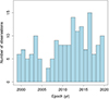 |
Fig. 1. Distribution of 164 observational epochs. |
The positions of C7 on the sky and their positional errors are shown in Fig. 2. Positional errors were estimated in directions along the positional angle relative to the core and transverse to it. The estimates of positional errors were obtained as in Arshakian et al. (2020) using the procedure suggested by Lampton et al. (1976) and based on minimising the χ2 statistics. The median standard errors of C7 positions along and across the jet axis are δj ≈ 4.8 μas and δn ≈ 1.5 μas, respectively. The measured errors are treated as lower limits, while the true errors can be higher by a factor of a few. They also estimated the flux leakage effect between the radio core and C7 and concluded that it is typically small, within 10%. Throughout the paper, we assume that the measured positional uncertainties are close to proper errors.
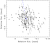 |
Fig. 2. Scatter of 164 positions of C7 on the sky plane. The sizes of the crosses correspond to C7 positional errors in the directions towards and across the core. The median position of the scatter is marked by a blue plus sign. The dashed blue line connects the median position of C7 and the core. |
We verified this assumption by using the AIPS task UVMOD (Greisen 2003) to create 20 simulated VLBA epochs using homogeneous sphere models based on real BL Lacertae structure and noise levels, randomised for (u, v)-coverage and epoch. The simulations were model-fit by another member of our team who did not know the location of C7 in each simulation. A comparison of the fitted location with known simulated C7 positions revealed standard deviations of 5.0 μas and 2.7 μas in the declination (Dec) and right-ascension (RA) directions, respectively, which are very similar to the estimated uncertainties given above.
3. Trajectory analysis of quasi-stationary component
The compact radio core of the jet is usually the brightest feature when analysing images from VLBA observations and is used as a reference point for measuring the angular distances to the radio components of the jet. Measuring the distance between the core and C7 at different epochs allows us to study the dynamics of C7 and for this purpose Arshakian et al. (2020) introduced the apparent displacement vector, r, which defines the direction of motion of C7 between two consecutive epochs, t and t + Δt, and the length of the displacement, r = |r|. If the radio core has proper motion, the measured apparent displacement of C7 is a combination of the radio core displacement (c) and the C7 proper motion (s). The distributions of apparent displacements and their errors, δr, which were calculated by propagating the positional uncertainties of C7 at two consecutive epochs, are similar to those in Arshakian et al. (2020). The median displacement and its mean error are 0.028 mas and 0.008 mas, respectively.
Arshakian et al. (2020) found that the larger displacement vectors have a tendency to be aligned along the jet axis. They interpret this as evidence of the radio core wiggling along the jet axis due to changes in the physical conditions in the core region, which in turn scatters the intrinsic positions of C7 along the jet axis, and developed a method to estimate the intrinsic mean and standard deviation of the core and C7 displacements. The mean displacement of the core is  and standard deviation σc = 0.025 mas, while the intrinsic motion of the C7 has a mean value of
  mas and σs = 0.012 mas. They conclude that both the anisotropic motion of the core and the intrinsic motion of C7 make a comparable contribution to the apparent motion of C7. Here, we assume that the apparent motion of C7 is mainly due to the anisotropic motion of the core and the intrinsic motion of C7.
3.1. Optimal time interval of a sliding window for the moving average procedure
To study the dynamics of the C7 intrinsic motion, we need to reduce the contribution of anisotropic core displacements, which have been shown to occur along the jet axis (Arshakian et al. 2020), and treat the asymmetric errors of the C7 positions. We used a moving average method that averages the anisotropic random motion of the radio core and any random C7 motions over a given time interval. For each epoch, the moving average procedure computes the average position of C7 and its error over a given time interval. The choice of the time interval of the sliding window should be optimal to average out the effects of the core displacement and at the same time preserve as far as possible the intrinsic trajectories of C7. For this purpose, we analysed the changes in the Dec of C7 with time. The effect of the core displacement should be stronger along the Dec axis than along the RA axis (Fig. 3), because the direction of the central axis of the jet (PAjet = −169°), along which the core wiggles, almost coincides with the Dec axis. Indeed, the change in the position along the Dec axis (bottom panel) shows stronger variation on scales of observing time intervals. The width of a sliding window should include several ups and downs for a reasonable smoothing of core displacements. Otherwise, the smoothing curve will follow the ups and downs, which means that the core effect is not well smoothed. The quasi-oscillatory changes in C7’s position between 2015.5 and 2019 happen on timescales of about 1 yr (Fig. 3, bottom panel). It is unclear whether these changes are due to the effect of core displacement and/or intrinsic changes in C7’s position. To properly smooth these quasi-oscillatory changes, the averaging time interval should be of the order of about one year – the timescale of the quasi-oscillatory changes.
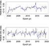 |
Fig. 3. Change in RA and Dec with epoch (black line). Smoothing was done with the moving average procedure using the fixed time interval of 1 yr (blue line). |
Another estimate of the timescales of cores displacements comes from consideration of the ejection rate of moving components. Core displacements happen due to particle density and magnetic fields changes as well as brightening of the core due to the passage of moving radio components through the core, as the region where opacity reaches τ = 1. For the BL Lac, the latter happens about once per year (Lister et al. 2021). If the moving component is brighter than the core (e.g. as a result of the injection of denser plasma into the jet stream (Plavin et al. 2019)), the inner region of the jet in the very long baseline interferometry (VLBI) image becomes elongated downstream with the brighter head displaced from the position of the core, resulting in an apparent displacement of the core. This suggests that the optimal smoothing time interval of Δtopt = 1 yr is indeed a reasonable choice.
In the BL Lac case, the propagating density perturbation of the jet plasma reaches the recollimation region (C7) from the core at 15 GHz after about four months (Arshakian et al. 2020), and its passage through the standing shock wave can affect its apparent motion in the direction of the jet axis both upstream and downstream. The timescale of these displacements should be comparable to the timescale of the core displacements; that is, of the order of one year or less. Therefore, we believe that a smoothing time interval of about one year will smooth out the apparent motion of C7 along the jet axis.
Another potential bias in the fitted position of the components, which could lead to apparent regular changes in the position of C7, could be the result of model fitting, where we feed up the source model taken from the previous epoch for the current one and let it relax. However, this approach is justified for the model fitting adopted in the MOJAVE program data analysis, as (i) every source in the MOJAVE sample has its individual observing cadence according to the rate of its morphological changes derived from initial observing epochs, and (ii) BL Lacertae is a record holder in terms of the number of observing epochs over all sources of the entire MOJAVE sample, with the highest cadence of one month. For a more detailed discussion of data reduction and model fitting, we refer the reader to Lister et al. (2009, 2018).
3.2. Smoothing the trajectory on timescale of one year
The trajectory of C7 smoothed by a moving average on timescales of about a year is shown in Fig. 4 for four time periods. The average number of epochs in a rolling window of one year is about nine. The moving average procedure reduces the number of epochs to 155. The mean position error is asymmetric and it is represented as an ellipse (Fig. 4) with the major axis directed to the core. The asymmetric 1σ position errors are represented by half of the major and minor axes.
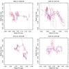 |
Fig. 4. Trajectory of C7 smoothed by the moving average procedure on a timescale of 1 yr (blue line). For clarity, the smoothed trajectory is represented for four time periods: 1999.37–2004.08, 2006.26–2013.42, 2013.42–2016.61, and 2016.61–2019.98. Average asymmetric positioning errors are shown by ellipses. The median scatter position over the whole time range from 1999.37 to 2019.98 is marked with a red plus sign. The dashed red line is the central axis of the jet connecting the median position of C7 and the radio core. |
It is evident that ellipse errors are intersecting along the displacement when it is small, which means that estimates of small displacements can be unreliable. For this, we assume that the measurement of displacement is unreliable if the error ellipses of two consecutive positions are intersecting along the displacement vector or 1σi + 1σi + 1 > ri. The algorithm based on this criterion compares the error ellipses between two consecutive positions. If the displacement between two consecutive positions is less than the sum of their 1σi and 1σi + 1 positioning errors along the displacement (when the error ellipses intersect), the position with the larger error is discarded, and the smaller position error is compared to the ellipse error of the next position; otherwise, if 1σi + 1σi + 1 ≤ ri then the ellipse errors σi + 1 and σi + 2 of the next two consecutive positions are compared. The application of this algorithm to the smoothed trajectory filters out about 60% of the positions. The resulting refined trajectory of C7 is shown in Fig. 5.
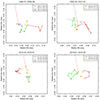 |
Fig. 5. Refined trajectory of C7 shown for four time intervals: 1999.37–2004.08, 2006.26–2013.42, 2013.42–2016.61, and 2016.61–2019.05. The arrows indicate the direction of movement. Red circles indicate reversal points for R- and RL-type; blue circles for A-type. Coloured sections of the trajectory indicate the path lengths of identified reversals and their combinations. The median scatter position over the whole time range from 1999.37 to 2019.98 is marked with a red plus sign. The dashed red line is the jet central axis, which connects the median position of C7 and the radio core. |
We now carry out a visual inspection of the refined trajectory. The component C7 starts in 1999.37 far from the median centre (plus sign) on the east side towards the median centre (red line), then makes a loop-like reversal at 2001.50 (yellow line) and moves to the south and sharply reverses at 2002.81 (green line). Notable is the long arcing movement to the northwest between 2002.81 and 2004.08 (yellow and green lines). There is a large gap in the observations between 2004.80 and 2006.26. After 2007.36, C7 moves in a long bending trajectory to the southeast and makes another sharp reversal at 2008.48 (red line). It shows a quasi-oscillatory clockwise (CW) motion between 2009.56 and 2011.70 (yellow line) and a sharp backward motion in 2012.48 (green line). Remarkably, starting around 2013.42, C7 begins its distinctive CW bending away from the centre in a westerly direction and then back towards the centre (red line). It reverses at 2014.66 to the south along the jet axis (yellow line). Also noteworthy is the large arc-like trajectory from 2016.61 to 2016.94 (red line), which reverses shortly before and makes a counterclockwise (CCW), near-oscillatory motion with an elongated orbit until late 2019 (green line). The whole trajectory of C7’s motion can be represented as a combination of reversible and arc-like motions on various timescales or spatial scales.
3.3. Reverse motion
The first step in analysing the motion of C7 is to check its randomness. If the motion of C7 is random, we should expect the number of angles between successive displacements with > 90° to be approximately equal to the number of angles with < 90°; that is, their ratio to be n(> 90 ° )/n(< 90 ° ) ≈ 1 for randomly directed displacements. This ratio is actually 2.5 times larger for angles estimated from the refined trajectory, 48/19 = 2.5. This suggests that the movement of C7 is not random, but rather directional, with alternating turns or reverse motion.
Another approach is to estimate the random probability of directional motion of C7: the probability that a sequence of k random displacement vectors lies within a given angle, ϕ. We simulated 160 displacements with an amplitude equal to one and a random orientation from 0 to 2π, and estimated the number of sequences of length k. We repeated this simulation 1000 times and estimated the average number of sequences of displacements,  . For example, we find that there are
  displacement sequences with three consecutive random displacements (k = 3) that are aligned within ϕ = 60°. The number of displacement sequences in the smoothed trajectory is n3 = 13, which is about three times larger and indicates that parts of the C7 trajectory are not random but rather directional in nature.
The general reverse motion is the key to understanding the nature of C7’s movement. Persistent reverse patterns are present on various spatial scales. To characterise the reverse motion, we distinguished between a reversible trajectory (R) with an angle ε ≤ 90° at the turning point and an arc-shaped reversal (RA) that has no inner turning point (ε > 90°). If an R-type motion formed a loop, we called it RL-type.
We defined the time at which the reversal occurs, ΔtR = te − ts, where ts and te are the start and end times of the reversal, respectively, and length of the reversal, ΔlR, between ts and te. The epoch at the pivot point of the reversal is denoted by tR.
In Table 1, we give 22 identifications of C7 trajectories. There are 21 reversing patterns with pivot points marked by circles in Fig. 5. Among them, 17 are R-type, 3 are RL-type, and 1 is RA-type (see Table 1). One trajectory between 2003.14 and 2004.08 (blue line) is identified as a probable RA-type reversal with an unknown epoch of a turning point. Most of the reversals are R-type. For clarity, we chose the likely epochs for the beginning and end of each reversal, ts and te, and have presented the trajectory of the reversals in different colours (Fig. 5). A clear R-shaped trajectory reversal at spatial scales of the order of 0.05–0.07 mas is observed between 2007.36 − 2009.15 (red line) and 2014.50 − 2014.96 (yellow line). We believe that a reversal of the same order occurs in an easterly direction with a pivot point at 1999.41 (red line), but we only observe its backward motion towards the median centre of C7 positions. There are 14 more R-type reversals on scales from about 0.01 to 0.05 mas (Table 2). We suppose that reversals on smaller scales are there but the scale of the smoothing interval (1 yr) and cleaning procedure puts a lower limit on the visibility of small reversals. A remarkable example of an arc-shaped reversal (RA-type) is observed between 2016.54 and 2016.94 (red line). Here, we assume that the reversal pivot point is at 2016.85, whose position is at the maximum distance from the starting position of the reversal. It is possible that a reversal of the same type occurs after 2003.14 (blue line), but the paucity of data at the threshold of the observational gap does not allow us to draw a decisive conclusion.
Characteristics of reverse motion.
Among the 22 reversals (Table 1), 13 are CW and 9 are CCW. This difference is statistically insignificant, and we assume that the direction of rotation of reversals is random.
We measured the radial distances, dr, between the pivot points of reversals and the median centre of the scatter of C7 positions. The radial distances of the reversal points are mainly in the range of 0.003 mas to 0.037 mas, with an average radial distance of about 0.025 ± 0.004 mas (see Fig. 6). The distribution of radial distances to the reversal points with CCW motion (shaded area) is not statistically different from the one for those with CW motion. The azimuthal angles of the turning points were measured with respect to the jet axis (CCW). There is a lack of turning points between 90° and 180°, which may be due to the small number of angle statistics. The CW and CCW reversals have similar distributions; that is, their pivot points occur in random directions.
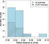 |
Fig. 6. Distribution of radial distances of 21 turning points from the median position of the C7 scatter. The shaded area shows the distribution of radial distances of the turning points of reversals with CCW motion. |
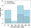 |
Fig. 7. Distribution of azimuthal angles for 21 turning points. The shaded area shows the distribution of azimuthal angles of the turning points of reversals with CCW motion. |
We measured 18 time intervals between pivots of successive reversals, Δτ (three time intervals were excluded from the statistics: one time interval due to the uncertain epoch of the turning point of the RA-type reversal and two time intervals between 2002.81 and 2008.48 due to the observation gap). They have a fairly flat distribution within the range of 0.03–1.34 yr and a mean value of  yr, which corresponds to a reversal frequency of fR ≈ 1.5 yr−1.
Combination of reversals. We observe reversible trajectories consisting of a combination of smaller reversals (or sub-reversals). For example, three consecutive reversals – two R-type with vertices at 2002.52 and 2002.60 and one RL reversal at 2002.81 (three red circles in Fig. 5; Table 1) – have two common displacements, and spatial scales of about 0.012, 0.011, and 0.008 mas, respectively, and two of them have reversal angles close to 90°. We assume that all three reversals are part of a large reversal occurring between 2001.79 and 2003.14 (see the green line in Fig. 5 and Table 2) with a turning point at 2002.81, which is the furthest from the initial onset of the reversal. Three analogous small-scale reversals, manifesting within spatial scales below 0.01 mas, contribute to a large R-type reversal observed between 2013.42 and 2014.50. The latter comprises two R-type reversals and one RL-type reversal, occurring, respectively, at 2013.61, 2013.64, and 2013.96 (red circles). Notably, 2013.61 is the furthest reversal point from the initial onset, and is thus designated as the primary pivot point (Fig. 5; Table 1). We call a reversal consisting of a combination of sub-reversals an RC-type.
Characteristics of reversals and reversal combinations. The latter are marked with a grey bar.
We identify another type of reversal combination, such as the trajectory between 2009.56 and 2011.70 (yellow line), which exhibits a quasi-oscillatory motion consisting of two R-type reversals and one RL-type reversal on a small spatial scale of 0.012 mas (Table 2). This is consistent with the small amplitude of the transverse jet wave (≈0.02 mas) during the period of low jet activity between 2010 and 2012 (Cohen et al. 2015; Arshakian et al. 2020). A similar quasi-oscillatory trajectory is observed between 2017.65 and 2019.05 (green line) on timescales of about 0.03 mas, which consists of one RL- and two R-type reversals at turning points 2018.52 and 2018.86. The combination of reversals exhibiting quasi-oscillatory motion is labelled as RO-type. Notably, RO-reversals consist of sub-reversals with the same direction of motion, CW or CCW (see Table 1).
We estimate the apparent speeds of C7 during reverse motion as βs* = ΔlR/ΔtR, and they range from 0.03 c to 0.77 c (Table 2). These subluminal speeds are actually lower limits as the ΔlR distances decrease due to smoothing of the C7 trajectory on timescales of one year. For the same reason, the spatial scales of reversals, which are estimated as the maximum reversal size, represent lower limits. The highest speed (0.77 c) of C7 is observed for the RA-type reversal (red line between 2016.61 and 2016.94 and Table 2), while the lowest speed of 0.03 c is estimated for the R-type reversal. It is noteworthy that both reversals occur at a spatial scale of 0.03 mas. The average time interval of the R and RL reversals is about 1.1 ± 0.2 yr, which is about three times that of one RA type. As for the four combined reversals, the average time interval is about 1.2 yr and 1.8 yr for the two RC and two RO types, respectively. Additional statistics for RA, RC, and RO types are needed to confirm these data. We also compared the distributions of time intervals ΔtR for CW and CCW reversals and found no significant difference.
To test whether the results of Sect. 3 hold for a smoothing time interval longer than the optimal interval of one year, we repeated the analysis of this section for a smoothing time interval of 1.5 yr. The number of reversals decreased from 22 to 12 with an equal number of CW and CCW movements (Table 1). The ratio characterising the directional motion of C7 becomes larger, n(> 90 ° )/n(< 90 ° ) = 38/12 ≈ 3, indicating that the movement of C7 is not random. All seven reversals on timescales of ≳1.5 years were preserved (Table 2). Among them there are three R-type, two RO-type, one RC, and one RL-type in 2001.5, which changed to R-type after smoothing. The remaining reversals are R-type (or change to it) on timescales of > 0.3 year. Thus, the C7 movement is directional, the reversals persist mainly on longer timescales, and the directions of the reversals are random. We conclude that the main results of this section remain unchanged.
4. Model for reversible motion
Cohen et al. (2015) report a close correlation between C7 position angles and the jet ridge line. Based on this relationship, they suggest that C7 excites transverse waves that propagate downstream from the jet with relativistic speeds. Arshakian et al. (2020) show a correspondence between the spatial scales of C7 motion and the amplitudes of relativistic transverse waves. In this study, we have shown that C7 performs reversible motion on different spatial scales. This suggests that the reversible motion of the stationary component of C7 is a projection of its motion along the transverse wave of the jet. Here, we assume that transverse waves are generated up to C7 upstream of the jet. In this case, the passage of the wave through the location of C7 causes it to make oscillatory motions across the jet, similar to the motion of a boat at anchor on a wave. Depending on the geometry of the wave, reversible motions of different types can be observed. If we consider a simple case in which the line of sight coincides with the central axis of the jet and the wave propagates in the plane passing through the line of sight, then the motion of the wave along the axis of the jet will shift the stationary component C7 across the jet axis. If the wave is periodic, then C7 will oscillate transverse to the axis and the observer will register a linear reversal motion of C7. Such a linear reversal motion can also be observed if the jet axis makes some angle with respect to the line of sight and the plane of the wave passes through the jet axis and the line of sight (or close to them). In this case, the direction of the linear reversal should be parallel (or nearly parallel) to the jet axis, as for example in the case of the reversal occurring between 2007.36 and 2009.15 (Fig. 5, red line). In most cases, the reversal motions of C7 are not linear, indicating that the waves have a twist in three-dimensional space; that is, a swirling structure. If the wave is periodic and the twist angle is constant, C7 exhibits quasi-circular motion (like the yellow line between 2009.56 and 2011.70 and the green line between 2017.65 and 2019.05) if the jet is viewed within the jet opening angle, and ellipse-like motion (e.g. green line in 2011.70–2013.42) when the jet viewing angle is larger than the jet opening angle. Certain combinations of wave twist angle, wave twist direction, and jet viewing angle can lead to looping reversals, such as the RL-type reversal observed during 2000.01–2001.79.
In this scenario, the passage of the wave through the C7 position moves the latter from the wave trough down the slope towards the crest, round the crest, and then towards the wave trough. This movement of C7 is observed as a reversible movement with a pivot point at the wave ridge position. Each observed reversal corresponds to a transverse wave passing through C7; hence, the mean transverse wave frequency, fw = fR = 1.5 yr−1, and mean wave period,  yr. We defined the wave amplitude, Aw, as the distances from the pivot point to the midpoint of the distance between the initial and final positions of the reversal. We used the measured spatial scales of the reversals (Table 2) as a proxy for their amplitudes. There is a small deviation between the two for reversals with large angles at the turning points (see, e.g., Fig. 5, yellow line between 2014.50 and 2014.96), but for the other reversals the deviation is negligible. The most energetic waves with large amplitudes of Aw ∼ 0.05 mas belong to the R-type, and conversely the weakest waves have small amplitudes of the order of 0.01 mas and appear as different types, R and RO. The speed of C7 in the reference frame of the host galaxy depends on the velocity of the transverse wave and wave’s twist at the position of C7. In the next section, we detail the apparent speeds of C7 measured by the observer in the context of the proposed C7 model.
5. Superluminal speeds of quasi-stationary component
Arshakian et al. (2020) estimated 111 transverse speeds of C7. The mean apparent speed was found to be superluminal,  , with ≈90% of the speeds larger than the speed of the light (this fraction holds also for the 163 transverse speeds measured in this study). They attributed this to significant core displacements and used projections of the C7 displacements onto the axis transverse to the jet, which is unbiased (i.e. free of core displacement effects), to estimate the C7 apparent speeds and found that the lower limits of most speeds, βs > 1.2 c, still remain superluminal. It remained unclear why the speeds of the QSC, which moves in a plane almost normal to the jet axis, should be superluminal. To register superluminal speeds, there must be a relativistic component that moves at a small angle to the line of sight. We assume that the transverse wave of the jet moving with relativistic speed at a small viewing angle shifts the QSC in the transverse direction from the jet with subluminal speed, which in the observer’s rest frame is registered as superluminal. For simplicity, we assume that the wave propagates in the sagittal plane (the plane containing the line of sight and the central axis of the jet; see Fig. 6 in Cohen et al. 2015). The sagittal plane is shown in Fig. 8 when viewed from a direction normal to the sagittal plane.
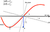 |
Fig. 8. Sketch of the apparent transverse motion of the QSC C7 (CB) as the relativistic transverse wave travels along the jet axis (AB). The jet axis makes an angle, θ, to the line of sight. |
Assuming that the QSC is located at the intersection of the transverse wave and the jet axis at point C: while the wave propagates along the jet central axis with relativistic speed,  (in the frame of a host galaxy), and passes the distance
  in the longitudinal direction in a time interval, δtg, the C7 travels a distance,
  , in the direction transverse to the jet axis with a speed of
  . We let θ be the viewing angle of the jet along the central axis. An observer measures the displacement of C7 (rs = rs, tr cos θ) over time, δt, and hence the apparent transverse velocity of C7, βs = rs/δt. Given that
  and relativistic time transformation of
  , we obtain an expression for the transverse velocity of C7 in the frame of a host galaxy,
 (1)
(1)
We consider the ratio
 (2)
(2)
where φ is the wave twist angle; that is, the angle between the wave tangent and the direction of the jet central axis, which ranges from 0° to φmax < 90°. Using Eq. (2), we invert Eq. () to express the apparent transverse speed of C7 measured by the observer,
 (3)
(3)
If the wave propagates in a plane perpendicular to the sagittal plane, the transverse motion vector of the C7 makes a right angle to the line of sight and remains so irrespective of changing the viewing angle. In this case,  and Eq. (3) transforms to
 (4)
(4)
The apparent speeds of the same waves propagating in the sagittal plane and normal to the sagittal plane (Eqs. (3) and (4)) may differ substantially if the viewing angle is large. For small θ < 10° (Cohen et al. 2015; Pushkarev et al. 2017; Homan et al. 2021), the speed difference is negligible.
Transverse wave speeds. Cohen et al. (2015) estimated the longitudinal speeds of four transverse waves adopting θ = 6° (see their Table 1). They used the shift of ridge lines in time at a distance of about 2–3 mas from the radio core. All transverse waves have relativistic speeds and are in the range of  , which corresponds to the range of Lorentz factors, Γwave = 3.5 − 15. We assume that transverse waves have the same speeds at a time when passing C7. The change in βs as a function of φ and
  for the fastest and slowest transverse waves,
  and
and  (Fig. 9, full and dashed lines).
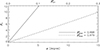 |
Fig. 9. Apparent transverse velocity, βs, of C7 as a function of the wave twist angle, φ, and transverse velocity, |


The transverse speed,  , of C7 depends on the wave speed,
  , and its twist angle, φ. The fastest wave (full line) with slopes > 0.5° moves C7 with subrelativistic speeds,
  , which appear to be superluminal with βs > 1 in the observer frame. In the case of the slowest transverse wave (dashed line), the wave twist angle and transverse velocity of C7 must be three times larger, ≈1.5° and ≈0.03 c, to measure apparent speeds exceeding the speed of light. We estimate the mean and dispersion of apparent speeds of C7 to be βs = 9.32 ± 0.96 and σβs = 8.06 for smaller observing intervals less than a month, implying that the latter describe more realistic trajectories. Then, possible transverse speeds of C7 and twist angles of waves lie in the ranges (0.08 − 0.28) c and 4 ° −14°, respectively (see Fig. 9). It should be noted that these estimates are obtained for the case when the transverse wave propagates in the sagittal plane, which causes C7 to perform a linear reversing movement along the jet axis. An example close to such a movement is the linear reversal marked in red between 2007.36 and 2009.15 (Fig. 5). In fact, in most cases we observe non-linear reversals, indicating that the plane of the transverse waves makes some angle with the sagittal plane and/or the transverse waves have a twist in space. Thus, our speed estimates should be taken as evidence that relativistic transverse waves are capable of producing the apparent superluminal speeds of C7.
Intrinsic apparent speed of C7. The transverse velocity of C7 in the frame of the host galaxy,  , is a function of the velocity of a transverse wave, the C7 intrinsic apparent transverse velocity, and the viewing angle of the jet (Eq. ()). To estimate
  , we adopted θ = 6° and the range of transverse wave speeds discussed above,
  . The intrinsic apparent speeds, βs = rs/Δt, cannot be directly measured, but their statistical characteristics such as the mean
  and standard deviation σβs can be estimated. We used the statistical approach developed in Arshakian et al. (2020) to estimate the unbiased mean and standard deviation of C7 displacements from their Eqs. (9,10):
 (5)
(5)
and
 (6)
(6)
where  is the mean of the measured displacement projections transverse to the jet central axis and
  is the mean of the rn squared. They argued that more realistic displacements are those with smaller observation intervals, Δt < 35 days, and used them to estimate the
  mas and σrs = 0.011 mas for 54 observational intervals (see their Table 1). Adopting the same constraint, we chose 63 of the 163 observation intervals in our sample and obtained the same values for
  and σrs and the mean observation interval
  yr and σΔt = 0.026 yr. Then, the C7 mean apparent speed,
  , is superluminal with σβs = 1.13 using the error propagation in the ratio. For 35 shorter observation intervals limited to Δt < 20 days, the mean speed is
  and σβs = 1.98. For our analysis, we adopted the latter values as more realistic.
The mean apparent speed of C7  corresponds to a mean speed of
  and
and  in the host galaxy frame (Fig. 9). Given
  variation in mean speed, we measured ranges of
  and
and  . The upper limits of the twist angles and speeds of φ ≲ 12° and
  (the latter is still subluminal) are given at a 3σβs ≈ 6 level. If the apparent speed is subluminal βs < 1, then φ ≲ 1.5° and
  . We note that these estimates are model-dependent and may vary with changes in the values adopted for the transverse wave velocity and jet viewing angle.
6. Discussion
The averaging filter and trajectory refinement algorithm smooth the structures on spatial scales of ≲0.01 mas. Because of the asymmetric positioning errors of C7, refinement of its trajectory affects structures extended in the jet direction to a greater extent than those in the transverse jet direction. For example, the turn enveloping the median centre of C7 positions is elongated in the jet direction (upper left panel in Fig. 4), and, after trajectory refinement, the reversal turns into an arc-shaped trajectory (upper left panel in Fig. 5). The refinement procedure can affect the reversal type; for example, changing it from RL- to R-type, as in the case of an R-type reversal (red line in the upper right panel of Fig. 5) that looked like an RL-type before refinement (upper right panel of Fig. 5). Trajectory refinement does not affect the direction (CW or CCW) of the reversal.
The jet ridge line and moving components appear downstream from C7, the median position of which is at a distance of 0.26 mas from the 15 GHz core (Cohen et al. 2014, 2015). At high resolution based on a single epoch observation at 86 GHz, the jet ridge line is detected up to a projected distance of about 0.4 mas from the core (Kim et al. 2023). We believe that the component at the core separation of approximately 0.3 mas is the C7 QSC. The reasoning behind this is that this component is the brightest feature in the 86 GHz jet beyond 0.1 mas from the core and is situated at the expected core separation, taking into account the frequency-dependent core shift effect (e.g. Lobanov 1998; Sokolovsky et al. 2011; Pushkarev et al. 2012). The jet at 86 GHz has a complex structure with multiple bends within 0.4 mas from the core. This suggests that the transverse waves are generated upstream of C7 and become visible at 15 GHz downstream of C7. The magnetic fields upstream and downstream of C7 have a strong toroidal component, indicating that there is a dense spiral field at sub-parsec (Kim et al. 2023) and parsec scales (Pushkarev et al. 2023), and that the magnetic field still dominates the jet dynamics at these scales. This argues in favour of a magnetohydrodynamic (MHD) wave model (Meier et al. 2001) in which C7 is the ‘master’ recollimation shock wave, while the moving jet components are compressions of slow and fast magnetosonic waves generated beyond the recollimation shock (Cohen et al. 2014, and references therein), and the transverse patterns of the ridge line are Alfvén MHD waves excited by C7 (Cohen et al. 2015). The latter is analogous to the excitation of a wave on a whip by shaking the handle. The C7 model proposed in Sect. 4 assumes that the transverse waves are generated upstream of C7, somewhere between the base of the jet and C7. This diverges from the shaking whip model, where C7 is the site of wave excitation.
Disturbance of the plasma across the jet leads to the excitation of transverse Alfvén waves (Gurnett & Bhattacharjee 2005) that propagate downstream at relativistic speed, similar to hose waves excited under high pressure. In favour of this scenario is the random nature of the twisting wave direction (or reversal direction) discussed earlier. The characteristics of the jet wave, such as amplitude, velocity, and frequency of generation, depend on the characteristics of the toroidal magnetic fields and the jet plasma.
We assume that during the active state of the jet, powerful transverse waves with large amplitudes of ≲0.05 mas are generated, which we observe as irregular C7 reversal patterns in random directions across the jet. When the plasma disturbance weaken, the steady state of the jet comes in the form of quasi-oscillatory waves with an amplitude ≲0.02 mas during 2010–2012 (Cohen et al. 2015; Arshakian et al. 2020), which we observe as quasi-oscillatory C7 motion on spatial scales of ≈0.01 mas between 2009.56 and 2011.70 (see the yellow line in Fig. 5 and Table 2). We speculate that the quasi-oscillatory waves observed during the steady state of the jet reflect the wobbling of the inner jet near the accretion disc, as is seen in three-dimensional MHD simulations of the black hole-accretion disc-jet system (McKinney et al. 2013). Modelling of relativistic MHD waves is necessary to shed light on the physical conditions of the plasma and magnetic field configuration required for the transition from the stable jet state to the active jet state, and to determine the region of wave excitation.
The excited Alfvén waves propagate along the spiral magnetic ‘muzzle’ of the jet and pass through the location of the recollimation shock wave C7. In this scenario, C7 acts as a jet nozzle whose dynamics and direction are controlled by transverse wave characteristics such as amplitude, twist angle, and velocity. The brightness of C7 depends on the intrinsic brightness of the jet beam, its velocity, and the viewing angle of the jet at the C7 position (Arshakian et al. 2020). The latter varies with the angle of wave twist at C7. Downstream of C7, the jet opening angle is about 4°, and the shape is parabolic, which changes to conical at a distance of 2.5 mas (∼3 pc) from the core (Pushkarev et al. 2017; Kovalev et al. 2020). The size of the C7 positional spread (∼0.1 mas) is determined by the maximum amplitude of the transverse wave (∼0.05 mas).
The advantage of studying QSCs in light of the new model is that the C7 characteristics allow us to study the transverse jet wave dynamics at small spatial scales, which are unattainable when analysing smoothed jet ridge lines (Cohen et al. 2014), as it is constructed in the image domain, while in this work we derive the positions of C7 from the data in the Fourier plane achieving significantly higher effective resolution. We believe that the study of the dynamics and brightness variations of the QSC can give detailed physical and statistical characterizations of relativistic transverse waves. The QSC dynamics can be strongly influenced by the effect of the core displacements. It is desirable that the dispersion of the core displacements be relatively small compared to the mean intrinsic displacement of the QSC. This allows us to use smaller smoothing intervals, and hence to study the dynamics on small temporal and spatial scales. If a QSC is too close to the core, a flux density leakage can easily occur between them, affecting the model fitting results by increasing the corresponding uncertainties. Therefore, to effectively study the dynamics of the QSC, it should be compact and bright, leading to small position errors, and have long-term VLBI observations with periods of significantly high cadence to study the dynamics on different timescales and assess the true position errors based on results from the nearest observing epochs.
7. Summary
We have studied the intrinsic trajectory of the QSC of the jet in BL Lac on sub-parsec scales using 164 epochs of observations made with the VLBA at 15 GHz over 20 years within the MOJAVE and VLBA 2 cm Survey. We highlight the following key results:
-
To recover the C7 intrinsic trajectory, we applied a moving average procedure to the apparent C7 trajectory, which smooths out the effect of the core displacement caused by the non-stationary nature of the jet. The optimal smoothing interval is about one year.
-
The overall smoothed and refined C7 trajectory is a sequence of reversible trajectories of different spatial scales. We identified 22 reversals, most of which are of R-type. Reversal motion occurs on average every 1.5 years. The number of reversals with CW and CCW motion (13 and 9, respectively) suggests that the trajectory twist is random. The distributions of radial distances and azimuthal angles of reversal turn points are not statistically different for CW and CCW reversals. We determined that a combination of successive reversals can form a larger RC-type reversal or a quasi-oscillatory trajectory identified as an RO-type reversal.
-
To describe the reversible motion of C7, we propose a model in which C7 is a standing recollimation shock wave and its dynamics is governed by the passage of relativistic transverse waves (Alfvén waves) through the stationary component of C7, which moves in a plane normal to the central axis of the jet, similar to the motion of a seagull on a wave. In the active state of the jet, irregular transverse waves with random twist are excited. The jet stabilises into quasi-oscillatory waves with regular twist, which is observed as a quasi-oscillatory motion of C7. We estimate the mean wave frequency to be about 1.5 per year, which is the upper limit. The amplitude of the transverse waves ranges approximately from 0.01 to 0.05 mas (0.013 − 0.065 pc).
-
The measured mean superluminal speeds of C7 can be understood within the framework of the proposed model. The relativistic transverse wave moves C7 at subluminal speed (∼0.04 c) in the host galaxy’s reference frame, while the observer detects it as superluminal, ∼2 c. The apparent transverse speed of C7 is superluminal for a maximum wave speed of 0.998 c (or Lorentz factor, Γwave = 15) and wave twist angle at the C7 position of ≳0.5°.
-
Important implications of the C7 model are that relativistic transverse waves are generated upstream of QSC and are mostly twisted in space, and the dynamics and kinematics of the QSC are determined by the speed, amplitude, and twist angle of the transverse wave, the maximum wave amplitude is about half of the QSC scattering size, and the superluminal speeds of the QSC indicate the presence of relativistic transverse waves in the jet.
Acknowledgments
We thank Yuri Y. Kovalev, Andrei Lobanov and Eduardo Ros for valuable comments and discussions. The VLBA is a facility of the National Radio Astronomy Observatory, a facility of the National Science Foundation that is operated under cooperative agreement with Associated Universities, Inc. This research has made use of data from the MOJAVE database that is maintained by the MOJAVE team (Lister et al. 2018). The research was supported by the YSU, in the frames of the internal grant. A.B.P. is supported in the framework of the State project “Science” by the Ministry of Science and Higher Education of the Russian Federation under the contract 075-15-2024-541.
References
- Arshakian, T. G., Pushkarev, A. B., Lister, M. L., & Savolainen, T. 2020, A&A, 640, A62 [EDP Sciences] [Google Scholar]
- Cohen, M. H., Meier, D. L., Arshakian, T. G., et al. 2014, ApJ, 787, 151 [Google Scholar]
- Cohen, M. H., Meier, D. L., Arshakian, T. G., et al. 2015, ApJ, 803, 3 [Google Scholar]
- Greisen, E. W. 2003, Astrophys. Space Sci. Lib., 285, 109 [NASA ADS] [Google Scholar]
- Gurnett, D. A., & Bhattacharjee, A. 2005, Introduction to Plasma Physics (Cambridge: Cambridge University Press) [CrossRef] [Google Scholar]
- Homan, D. C., Cohen, M. H., Hovatta, T., et al. 2021, ApJ, 923, 67 [NASA ADS] [CrossRef] [Google Scholar]
- Kellermann, K. I., Vermeulen, R. C., Zensus, J. A., & Cohen, M. H. 1998, AJ, 115, 1295 [NASA ADS] [CrossRef] [Google Scholar]
- Kim, D.-W., Janssen, M., Krichbaum, T. P., et al. 2023, A&A, 680, L3 [NASA ADS] [CrossRef] [EDP Sciences] [Google Scholar]
- Komatsu, E., Dunkley, J., Nolta, M. R., et al. 2009, ApJS, 180, 330 [NASA ADS] [CrossRef] [Google Scholar]
- Kovalev, Y. Y., Pushkarev, A. B., Nokhrina, E. E., et al. 2020, MNRAS, 495, 3576 [NASA ADS] [CrossRef] [Google Scholar]
- Lampton, M., Margon, B., & Bowyer, S. 1976, ApJ, 208, 177 [Google Scholar]
- Lister, M. L., Cohen, M. H., Homan, D. C., et al. 2009, AJ, 138, 1874 [NASA ADS] [CrossRef] [Google Scholar]
- Lister, M. L., Aller, M. F., Aller, H. D., et al. 2018, ApJS, 234, 12 [CrossRef] [Google Scholar]
- Lister, M. L., Homan, D. C., Kellermann, K. I., et al. 2021, ApJ, 923, 30 [NASA ADS] [CrossRef] [Google Scholar]
- Lobanov, A. P. 1998, A&A, 330, 79 [NASA ADS] [Google Scholar]
- McKinney, J. C., Tchekhovskoy, A., & Blandford, R. D. 2013, Science, 339, 49 [NASA ADS] [CrossRef] [Google Scholar]
- Meier, D. L., Koide, S., & Uchida, Y. 2001, Science, 291, 84 [Google Scholar]
- Plavin, A. V., Kovalev, Y. Y., Pushkarev, A. B., & Lobanov, A. P. 2019, MNRAS, 485, 1822 [Google Scholar]
- Pushkarev, A. B., Hovatta, T., Kovalev, Y. Y., et al. 2012, A&A, 545, A113 [NASA ADS] [CrossRef] [EDP Sciences] [Google Scholar]
- Pushkarev, A. B., Kovalev, Y. Y., Lister, M. L., & Savolainen, T. 2017, MNRAS, 468, 4992 [Google Scholar]
- Pushkarev, A. B., Aller, H. D., Aller, M. F., et al. 2023, MNRAS, 520, 6053 [NASA ADS] [CrossRef] [Google Scholar]
- Sokolovsky, K. V., Kovalev, Y. Y., Pushkarev, A. B., & Lobanov, A. P. 2011, A&A, 532, A38 [CrossRef] [EDP Sciences] [Google Scholar]
- Vermeulen, R. C., Ogle, P. M., Tran, H. D., et al. 1995, ApJ, 452, L5 [NASA ADS] [Google Scholar]
All Tables
Characteristics of reversals and reversal combinations. The latter are marked with a grey bar.
All Figures
|
Fig. 1. Distribution of 164 observational epochs. |
| In the text | |
|
Fig. 2. Scatter of 164 positions of C7 on the sky plane. The sizes of the crosses correspond to C7 positional errors in the directions towards and across the core. The median position of the scatter is marked by a blue plus sign. The dashed blue line connects the median position of C7 and the core. |
| In the text | |
|
Fig. 3. Change in RA and Dec with epoch (black line). Smoothing was done with the moving average procedure using the fixed time interval of 1 yr (blue line). |
| In the text | |
|
Fig. 4. Trajectory of C7 smoothed by the moving average procedure on a timescale of 1 yr (blue line). For clarity, the smoothed trajectory is represented for four time periods: 1999.37–2004.08, 2006.26–2013.42, 2013.42–2016.61, and 2016.61–2019.98. Average asymmetric positioning errors are shown by ellipses. The median scatter position over the whole time range from 1999.37 to 2019.98 is marked with a red plus sign. The dashed red line is the central axis of the jet connecting the median position of C7 and the radio core. |
| In the text | |
|
Fig. 5. Refined trajectory of C7 shown for four time intervals: 1999.37–2004.08, 2006.26–2013.42, 2013.42–2016.61, and 2016.61–2019.05. The arrows indicate the direction of movement. Red circles indicate reversal points for R- and RL-type; blue circles for A-type. Coloured sections of the trajectory indicate the path lengths of identified reversals and their combinations. The median scatter position over the whole time range from 1999.37 to 2019.98 is marked with a red plus sign. The dashed red line is the jet central axis, which connects the median position of C7 and the radio core. |
| In the text | |
|
Fig. 6. Distribution of radial distances of 21 turning points from the median position of the C7 scatter. The shaded area shows the distribution of radial distances of the turning points of reversals with CCW motion. |
| In the text | |
|
Fig. 7. Distribution of azimuthal angles for 21 turning points. The shaded area shows the distribution of azimuthal angles of the turning points of reversals with CCW motion. |
| In the text | |
|
Fig. 8. Sketch of the apparent transverse motion of the QSC C7 (CB) as the relativistic transverse wave travels along the jet axis (AB). The jet axis makes an angle, θ, to the line of sight. |
| In the text | |
|
Fig. 9. Apparent transverse velocity, βs, of C7 as a function of the wave twist angle, φ, and transverse velocity, |
| In the text | |
Current usage metrics show cumulative count of Article Views (full-text article views including HTML views, PDF and ePub downloads, according to the available data) and Abstracts Views on Vision4Press platform.
Data correspond to usage on the plateform after 2015. The current usage metrics is available 48-96 hours after online publication and is updated daily on week days.
Initial download of the metrics may take a while.