| Issue |
A&A
Volume 692, December 2024
|
|
|---|---|---|
| Article Number | A82 | |
| Number of page(s) | 14 | |
| Section | Planets, planetary systems, and small bodies | |
| DOI | https://doi.org/10.1051/0004-6361/202450549 | |
| Published online | 04 December 2024 | |
Detectability of biosignatures in warm, water-rich atmospheres
1
Institut für Planetenforschung (PF), Deutsches Zentrum für Luft- und Raumfahrt (DLR) „
Rutherfordstraße 2,
12489
Berlin,
Germany
2
Zentrum für Astronomie und Astrophysik (ZAA), Technische Universität Berlin (TUB),
Hardenbergstraße 36,
10623,
Berlin,
Germany
3
Institut für Methodik der Fernerkundung (IMF), German Aerospace Center (DLR),
82234
Wessling,
Germany
4
Institut für Geologische Wissenschaften, Freie Universität Berlin (FUB),
Malteserstraße 74-100,
12249
Berlin,
Germany
★ Corresponding author; benjamin.taysum@dlr.de
Received:
29
April
2024
Accepted:
22
October
2024
Context. Warm rocky exoplanets within the habitable zone of Sun-like stars are favoured targets for current and future missions. Theory indicates these planets could be wet at formation and remain habitable long enough for life to develop. However, it is unclear to what extent an early ocean on such worlds could influence the response of potential biosignatures.
Aims. In this work we test the climate-chemistry response, maintenance, and detectability of biosignatures in warm, water-rich atmospheres with Earth biomass fluxes within the framework of the planned LIFE mission.
Methods. We used the coupled climate-chemistry column model 1D-TERRA to simulate the composition of planetary atmospheres at different distances from the Sun, assuming Earth’s planetary parameters and evolution. We increased the incoming instellation by up to 50% in steps of 10%, corresponding to orbits of 1.00 to 0.82 AU. Simulations were performed with and without modern Earth’s biomass fluxes at the surface. Theoretical emission spectra of all simulations were produced using the GARLIC radiative transfer model. LIFEsim was then used to add noise to and simulate observations of these spectra to assess how biotic and abiotic atmospheres of Earth-like planets can be distinguished.
Results. Increasing instellation leads to surface water vapour pressures rising from 0.01 bar (1.31%, S = 1.0) to 0.61 bar (34.72%, S = 1.5). In the biotic scenarios, the ozone layer survives because hydrogen oxide reactions with nitrogen oxides prevent the net ozone chemical sink from increasing. Methane is strongly reduced for instellations that are 20% higher than that of the Earth due to the increased hydrogen oxide abundances and UV fluxes. Synthetic observations with LIFEsim, assuming a 2.0 m aperture and resolving power of a R = 50, show that ozone signatures at 9.6 µm reliably point to Earth-like biosphere surface fluxes of O2 only for systems within 10 parsecs. The differences in atmospheric temperature structures due to differing H2O profiles also enable observations at 15.0 µm to reliably identify planets with a CH4 surface flux equal to that of Earth’s biosphere. Increasing the aperture to 3.5 m and increasing instrument throughput to 15% increases this range to 22.5 pc.
Key words: Earth / planets and satellites: atmospheres / planets and satellites: detection / planets and satellites: terrestrial planets / planet-star interactions
© The Authors 2024
 Open Access article, published by EDP Sciences, under the terms of the Creative Commons Attribution License (https://creativecommons.org/licenses/by/4.0), which permits unrestricted use, distribution, and reproduction in any medium, provided the original work is properly cited.
This article is published in open access under the Subscribe to Open model. Subscribe to A&A to support open access publication.
1 Introduction
Rocky exoplanets in the inner habitable zone (IHZ) are at the cutting edge of exoplanetary research. Ongoing missions such as the Transiting Exoplanet Survey Satellite (TESS, Ricker et al. (2010)) are in the midst of discovering rocky planets in the so-called Venus Zone (Ostberg et al. 2023). These warm worlds have rather small orbital periods and will be discovered and characterised before their cooler counterparts in the middle and outer habitable zone. Furthermore, recently adopted missions to Venus by ESA (EnVision,Ghail et al. (2016)) and NASA (Veritas and DAVINCI; Smrekar et al. (2020), Garvin et al. (2022)) will also have a knock-on effect on exo-Venus research. Regarding volatile delivery, current theories suggest that rocky worlds forming in and around the IHZ of Sun-like stars will likely accrete water inventories that are broadly comparable with objects formed in the mid habitable zone (see e.g. Lammer et al. 2018). Recent studies (e.g. Way & Del Genio 2020; Höning et al. 2021) suggest an extended early habitability of Venus and Venus-like worlds (see e.g. Westall et al. 2023). The evolution of Venus-like planets and possible early habitability is a central issue in exoplanet science.
Current theory does not rule out modest, warm, water-rich atmospheres due to ocean evaporation as warm, rocky planets evolve through and beyond their habitable phase (Kasting 1993; Zahnle et al. 2010; Elkins-Tanton 2012). During early evolution, however, rocky exoplanets can feature giant, hot steam atmospheres, typically from the close of the magma ocean (MO) period when crustal formation leads to strong volatile out-gassing. These steam atmospheres are believed to play a crucial role in the early evolution of terrestrial planets and can eventually condense to form global oceans and hence lead to long-lived habitable conditions. Early Earth likely featured such a giant steam atmosphere at the close of its final MO period after the Moon-forming event (Elkins-Tanton 2008; Lebrun et al. 2013; Sossi et al. 2020; Gaillard et al. 2022; Sossi et al. 2023; Dorn & Lichtenberg 2021).
Regarding Venus, O’Rourke et al. (2023) recently reviewed planetary evolution and note that early climate runaway, and hence the timing and extent of a potential giant steam atmosphere phase, is likely sensitive to the global coverage and refractive properties of its clouds, which are not well known. For example, Salvador et al. (2023) reviewed water delivery and the blanket effect influencing the giant steam atmosphere climate on early Venus. Westall et al. (2023) reviewed Venus’s evolution, including volatile cycling and the consequences for long-term habitability. Lichtenegger et al. (2016) suggested that several hundred bars of steam atmosphere on early Venus could have been removed in the first 100 Myr, mainly due to non-thermal escape, depending on the uncertain extreme-UV flux of the early Sun. Way & Genio (2020) discuss the implications of the deuterium (2H) and protium (1H) ratio (D/H) data from Pioneer Venus, which suggest an extended shallow ocean on early Venus. The 3D model study by Turbet et al. (2021), however, suggests that the early Venusian giant steam atmosphere did not condense. Resolving these issues requires improved (more accurate and spatially extended) isotope and other proxy data, as discussed in, for example, Widemann et al. (2023).
Regarding rocky exoplanets, giant steam atmospheres are also likely during the early evolution. Their duration will depend on the interplay between, for example, outgassing, escape, and climate (which are not well determined) and could vary from several thousand to several million years after the close of the MO phase, as discussed in Nikolaou et al. (2019). Numerous studies have addressed the emergence, evolution, and climate of early, giant steam atmospheres by applying radiative-convective models. Abe & Matsui (1985) highlight the effectiveness of a steam-dominated atmosphere in thermally insulating the surface, but their assumption of a grey atmosphere (i.e. the absorption coefficients are assumed to be constant) led to an underestimation of surface warming. Kasting (1988) applied a 1D climate model to study the response of Earth-like atmospheres to large increases in instellation. More recently, Marcq et al. (2017) used a 1D radiative-convective model of H2O–CO2 atmospheres to study the thermal blanketing effect of steam atmospheres. Katyal et al. (2019, 2020) used a radiative-convective model to study the evolution of a steam atmosphere around the time of Earth’s final MO. Kite & Schaefer (2021) suggested that inward migrating sub-Neptunes can evolve into hot, rocky exoplanets and attain thick steam atmospheres from their original gas mantles. Harman et al. (2022) suggest that a 100 bar steam atmosphere on TOI-1266c could be detected with about 20 hours of observing time by the James Webb Space Telescope.
Earth-like atmospheric biosignatures and their responses to varying planetary and stellar parameters have been widely studied, for example: the response to the central star (e.g. Segura et al. 2005; Grenfell et al. 2007), the response over planetary evolution timescales (e.g. Gebauer et al. 2018; Rugheimer & Kaltenegger 2018), and the response to clouds (e.g. Kitzmann et al. 2011), to name but a few. None of these studies, however, investigated atmospheric biosignatures with consistent climate chemistry throughout the IHZ for conditions in which warm, water-rich atmospheres can form. Therefore, despite a rich, emerging literature focusing on, for example, early steam atmospheres in the Solar System and beyond, to our knowledge there are no dedicated climate-chemistry coupled studies for warm rocky exoplanets with water-rich atmospheres from evaporating oceans. Such models require flexible radiative transfer modules that can operate over a large range of atmospheres as well as comprehensive chemistry modules. Including coupled climate-chemistry models is important for three main reasons: (1) The gas-phase (photo)chemistry of water-rich atmospheres could directly affect atmospheric biosignatures; water-rich atmospheres can generate strong abundances of hydrogen oxides, HOX (=OH+HO2), via the photolytic breakdown of water by UV radiation. HOX can in turn destroy potential biosignatures such as ozone via catalytic cycles and methane via direct gas-phase reactions with the hydroxyl (OH) radical, which can also stabilise climate gases such as CO2 (Yung & DeMore 1998). (2) Via abiotic processes, steam can rapidly photolyse in the upper atmosphere. The resulting H atoms can be lost via escape, whereas the ground-state oxygen (O(3P)) atom is left behind. These oxygen atoms can self-react, leading to abiotic production of molecular oxygen and ozone (see e.g. Meadows 2017). (3) Due to UV shielding and climate blanketing, steam atmospheres shield UV and heat, which can directly affect photolysis and temperature-dependent gas-phase chemical reactions.
In this work we address these issues by performing coupled climate-chemistry model simulations of warm rocky planets with oceans for scenarios with and without Earth-like biospheres at the surface across the IHZ. These simulations produce high abundances (>10%) of water vapour at higher instellation runs.
2 Model and methods
2.1 Atmospheric column model, 1D-TERRA
1D-TERRA is a global-mean, stationary, coupled convective-climate-photochemical model consisting of one hundred layers extending from the planetary surface to 10−5 hPa. The convective-climate module (Scheucher et al. 2020) applies an adiabatic lapse rate in the lower atmosphere, with a convec-tive regime and radiative transport above according to the Schwarzschild criterium. The model is valid for pressures up to 1000 bar and temperatures up to 1000 K and can reproduce the atmospheric parameters and compositions of modern Earth, Venus, and Mars (Scheucher et al. 2020). The climate module uses the random overlap method for the frequency integration from 100 000 cm−1 (100 nm) to 0 cm−1 and the delta two-stream approximation for the angular integration. Up to 20 absorbing species in the visible/IR and 81 cross-sections in the UV-visible are available. The model includes Rayleigh scattering and the option to include self and foreign continua. Convective adjustment is considered applying the dry adiabat or the wet adiabat for H2O and CO2 condensibles and including adjustable ocean reservoirs (Manabe & Wetherald 1967).
The chemistry module from Wunderlich et al. (2020) features 1127 reactions for 128 species including photolysis for 81 absorbers. Dry and wet deposition as well as biomass, lightning (Chameides et al. 1977) and volcanic mass fluxes can be included flexibly. Adaptive eddy mixing depending on concentration and temperature profiles is employed, using the approach similar to Gao et al. (2015) that uses the equations developed by Gierasch & Conrath (1985).
2.2 1D-TERRA boundary parameters
Table 1 lists the surface fluxes, volcanic outgassing fluxes, and dry deposition velocities for trace gas species used in all model runs in this work. Surface fluxes deliver the species to the first model layer (centred at ~500 m) only, whereas volcanic fluxes are evenly distributed across the lower 10 km of the model domain. For all species except CO2 and O2, the surface fluxes are the sum of the modern Earth’s biogenic and anthropogenic emissions (Wunderlich et al. 2020). Volcanic outgassing fluxes are similarly representative of the modern Earth (Catling & Kasting 2017; Khalil & Rasmussen 1984; Etiope & Ciccioli 2009; Pyle & Mather 2009).
The values for CO2 and O2 surface fluxes were chosen such that the model run with a solar constant value of 1.0 approximately reproduces the modern Earth atmospheric CO2 and O2 abundances (355 ppm and 0.21 mol/mol, respectively). The negative flux used for CO2 represents surface uptake processes not included in our model involving, for example, biological and sub-surface processes.
1D-TERRA uses the Manabe-Wetherald relative humidity profile (Manabe & Wetherald 1967) in all simulations, which recreates the mean atmospheric water vapour profile of the modern Earth for a solar constant of 1.0 with a fixed surface relative humidity of 80%. The Chameides et al. (1977) lightning model was used to produce modern-Earth concentrations of NO and NO2 within the troposphere, and rainout rates of trace gas species were accounted for using the Giorgi & Chameides (1985) approach with effective Henry’s law constants via temperature-dependent parameterisations from Sander (2015).
Biomass surface fluxes, dry deposition velocities, and volcanic outgassing fluxes for trace gas species used in all model runs in this work.
2.3 GARLIC spectral model
GARLIC (General purpose Atmospheric Radiative transfer Line-by-line Infrared-microwave Code) was used to calculate theoretical transmission and emission spectra based on input of temperature and composition from 1D-TERRA output. GARLIC uses an optimised Voigt function with a three-grid approach for line-by-line modelling of molecular cross-sections using HITRAN or GEISA data as well as continua, collision induced absorption, and Rayleigh and aerosol extinction. The Jacobians (derivatives with respect to the unknowns of the atmospheric inverse problem) are constructed via automatic differentiation (Schreier et al. 2015). GARLIC has been validated via inter-comparison with other codes (Schreier et al. 2018a) and by comparing its synthetic spectra with observed spectra for modern Earth and Venus (Schreier et al. 2018b). Further details can be found in Schreier et al. (2014) and Schreier et al. (2019).
2.4 Scenarios
We modelled six scenarios with 1D-TERRA, simulating rocky exoplanets assuming Earth’s development and biomass across the IHZ (1.00 AU; scenario 1, S = 1.0) with instellation increasing at intervals of 0.1, resulting in S = 1.1 (0.95 AU, scenario 2), S = 1.2 (0.91 AU, scenario 3), S = 1.3 (0.88 AU, scenario 4), S = 1.4 (0.85 AU, scenario 5), and S = 1.5 (0.82 AU, scenario 6). To assess the impact of the active biosphere on the atmospheric biomarkers, the runs were repeated with all positive surface fluxes in Table 1 removed. The negative surface flux of CO2 was re-tuned to approximately reproduce the CO2 volume mixing ratio (VMR) of modern Earth for the abiotic S = 1.0 case. With less HOX in the mesosphere (pressures below approximately 0.01 hPa) from lower stratospheric H2O (discussed in Sect. 3.4), recycling of CO to CO2 via OH reactions is less efficient, and the lower CH4 content from surface biology lowers the rate of CO2 production from CH4 oxidation. An additional caveat is that without the uptake of CO2 from biological activity (e.g. photolysis, soil uptake) at the surface, abiotic planets with equal CO2 outgassing fluxes will result in greater CO2 atmospheric abundances than their biotic counterparts (Haqq-Misra et al. 2016). However, to focus on the atmospheric chemistry and responses appropriately, we chose to study biotic and abiotic worlds that possess the same atmospheric CO2 abundances. To achieve this, we lowered the CO2 surface flux to −2.286× 10⁹ molecules cm−2 s−1 for all the abiotic runs.
2.5 LIFEsim astrophysical noise generator
LIFEsim, developed by Dannert et al. (2022) and used in exo-planet retrieval studies such as Quanz et al. (2022), Konrad et al. (2022), and Alei et al. (2022), was used to add astrophysical noise signals to the emission spectra produced by the GARLIC radiative transfer code. The noise sources included are photon noise from stellar leakage, exozodi disks, the planet emission, and the local exozodi disk. Details of these noise sources are presented in Dannert et al. (2022) and Quanz et al. (2022). There is expected to be significantly less instrument noise than photon shot noise in the present version of LIFEsim, and it does not take instrument noise into consideration
The same simulation parameters used in Alei et al. (2022) are adopted in this manuscript, referred to as the ‘baseline’ LIFE scenario. This configuration is expected to be capable of measuring the emission spectra of Earth at a distance of 10 pc with a wavelength-integrated signal to noise ratio of 9.7 for a total measurement time of approximately 2.3 days (Dannert et al. 2022). The quantum efficiency of the interferometer’s detector is equal to 0.7, the wavelength range is set to 5.0–18.5 µm, the spectral resolution is R = 50, aperture diameter d = 2.0 m, and the exozodi level is set to 3 times that of the local zodiacal dust. LIFEsim is ran here across a grid of integration times (24, 48, 120, 240 hours) and distances from the Solar System (5–30 parsecs in intervals of 5 pc).
The statistical significance of the biotic signal at each wavelength band was calculated by dividing the absolute difference in retrieved flux for the biotic and abiotic scenarios by the noise calculated via LIFEsim (σBio):

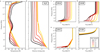 |
Fig. 1 Temperature (a), H2O vapour volume mixing ratio in mol/mol (b), and the UV-A (c), UV-B (d), UV-C (e), and FUV (f) fluxes calculated by 1D-TERRA for a (biotic) Earth-like planet with the mean incoming instellation increased from 1.0 (modern Earth) up by a factor of 1.5 (orbiting a Sun-like star at 0.82 AU). |
3 Results
Figure 1 shows 1D-TERRA output of atmospheric temperature (Kelvin, panel a) and water vapour (VMR; panel b) profiles, alongside the UV-A (λ = 317.5–405 nm), UV-B (λ = 281.7–317.5 nm), UV-C (λ = 175.0–281.7 nm), and far-UV (λ = 100.0–175.0 nm) radiation fluxes (W m−2; panels c–f, respectively). Regarding temperature, the stronger instellation leads to an increase in surface temperature from 287.7 K (scenario 1) to 365.4 K (scenario 6). The cold trap moves upwards due to expansion of the atmospheric column in the troposphere and becomes weaker. The adiabatic lapse rate in the lower atmosphere changes gradient because warmer temperatures lead to ocean evaporation, which modifies atmospheric composition and heat capacity. On increasing the instellation, firstly the temperature inversion (the rate of change of temperature with increasing altitude) is weakened. The inversion serves as a barrier to upward mixing, which acts as a ‘lid’ on the troposphere, preventing mixing of water upwards into the stratosphere; this barrier effect is therefore weakened and results in greater H2O quantities reaching the stratosphere. Secondly, the minimum temperature at the inversion increases from about 210 K (scenario 1) to about 250 K (scenario 6). This also suggests a weakening of the cold trap since it is less able to freeze out tropospheric water. The surface warming is accompanied by cooling in the middle atmosphere. This arises due to an enhanced classical greenhouse driven by increased ocean evaporation. Increasing H2O abundances within the troposphere trap heat with greater efficiency, decreasing the upward flux of long-wave radiation to altitudes above the tropopause whilst causing surface temperatures to rise. The lower flux of IR radiation entering the stratosphere that travels upwards from the troposphere causes regions with pressure below 10 hPa to cool, and the inversion layer to disappear by S = 1.4.
Regarding water vapour, the surface water VMRs range from 0.013 (PH2O = 0.01 bar) for S = 1.0 to 0.347 (PH2O = 0.6 bar) for S = 1.5 at the model surface. The increasing surface temperatures elevate the water vapour saturation pressures within the troposphere. As a fixed relative humidity of 80% is adopted within the troposphere, the resulting partial pressure of water vapour increases within the model. This approximates the effects expected from the evaporation of the Earth’s surface oceans as the surface temperatures progressively increase. At S = 1.5, a total surface pressure of about 1.6 bar occurs since we also assumed one bar of combined N2 and O2 for the modern Earth. On increasing instellation, the transition region from tropospheric water (with its adiabatic lapse rate) to stratospheric water (mainly affected by upward mixing and chemical production from methane oxidation) moves upwards due to expansion and results in a convex-shaped bulge for the higher instellations, associated with, for example, increasing upward water transport and due to the imposed Manabe–Wetherald relative humidity isoprofile.
UV-A radiation in Fig. 1 penetrates efficiently through the atmosphere down to about 100 hPA, below which higher pressures lead to its exponential absorption in all scenarios. UV-B is mainly absorbed by O3. The presence of Earth’s O3 layer centred at about 10 hPa (around 30km on modern Earth) effectively shields the surface from the incoming UV-B flux, resulting in the absorption ‘shoulder’ slope seen in Fig. 1d. In the free troposphere the flux gradient of UV-B increases more strongly with altitude for the higher instellation scenarios. This is likely related to the ozone response, as discussed in the next section. UV-C radiation decreases rapidly for scenarios S = 1.0 to S = 1.2 for pressures greater than about 100 hPa, mainly due to increasing water vapour and atmospheric pressure. For scenarios S = 1.3 to S = 1.5, however, the radiation is more efficient at penetrating down to the surface. This is related to the ozone response as discussed in the next section. Far-UV radiation is mainly absorbed in the mesosphere via water vapour for all scenarios.
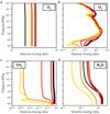 |
Fig. 2 Vertical distribution profiles of the VMRs of O2 (a), O3 (b), CH4 (c), and N2O (d) displayed in units of mol/mol for the biotic scenarios (see Fig. 1 for the colour legend). |
3.1 Climate-chemistry response of biosignatures
In this section, we analyse scenarios 1–6 (with biomass emissions) and describe the climate-chemistry response of atmospheric (potential) biosignatures in our model scenarios. Specifically, we analyse VMR profiles of O2, O3, CH4, and N2O in Figure 2.
3.1.1 O2
Despite the surface flux of O2 remaining constant (Earth’s biomass) for each model run (Table 1), the VMR of O2 steadily increases (Figure 2a) with an increase in solar constant, ranging from 0.20 for S = 1.0 to 0.35 for S = 1.3. At S = 1.4, this trend reverses, and O2 VMRs fall to 0.32 and then 0.25 mol/mol at S = 1.5. From S = 1.0–1.5, the corresponding partial pressures for O2 are 0.20, 0.29, 0.36, 0.42, 0.45, and 0.44 bars respectively – O2 production is therefore still increasing in rate up to S = 1.4 despite a drop in VMR. The dominant photochemical sink for O2 in all model runs is photolysis within the wavelength range λ = 10–200 nm above the troposphere. With an increasing solar constant, the photolysis rates of O2 steadily increase. However, the presence of more H2O vapour in the simulations with a higher solar constant introduces a greater abundance of HOX species, rising from < 1 pptv for S = 1.0 to 1–10 ppbv for S = 1.4 within regions of 100−10 hPa. This results in catalytic cycles driven by OH, HO2, and H to recycle O(3P) atoms (produced from the photodissociation of CO2, H2O, and O3) into O2 molecules increasing in rate faster than the rate of O2 photolysis, enabling the O2 VMR to rise with increasing solar constant. At S = 1.5, the UV-C radiation flux in the lower atmosphere is orders of magnitude larger due to the falling tropospheric O3 concentrations, and the O2 photolysis increases in rate faster than O2 is regenerated by the catalytic cycling of HOX compounds. Additional O2 is delivered from the top of the atmosphere due to the increasing escape rates of hydrogen and the photolysis of CO2, with the H escape flux reaching 0.69 Tg yr−1 for S = 1.5. The H escape flux enables the O atoms left behind react with OH and to stimulate the mesospheric abiotic O2 production without being lost to HOX cycles.
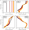 |
Fig. 3 Vertical distribution profiles of the VMRs of CO2 (a), the HOX group (b; see also Fig. A.1), the NOX group (c; see also Fig. A.2), and HNO3 (d) displayed in units of mol/mol for the biotic scenarios (see Fig. 1 for the colour legend). |
3.1.2 O3
An unexpected result of this work is that the bulk of the atmospheric O3, occurring mainly in the stratospheric ozone layer centred at about 10 hPa (Fig. 2b) mostly survives in all scenarios. Why? This result is not due to stronger O2 photolysis stimulating the Chapman cycle, since the necessary UV-C fluxes are not strongly enhanced in the middle stratosphere (Fig. 1e) for the increased instellation scenarios but are instead efficiently absorbed. The survival of stratospheric O3 is all the more puzzling when one notes that UV-B, a photolytic sink for O3, is actually enhanced with increasing instellation (Fig. 1d). Results in the stratosphere suggest that HOX is strongly increased as expected for the high instellation scenarios with enhanced steam (Figs. 3b and A.1). However, the increased HOX can act as a sink for NOX and ClOX, and, importantly, this occurs in the regions where these species would otherwise strongly remove ozone catalytically, that is, in the lower stratosphere (NOX; Figs. 3c and A.2) and the mesospheric (ClOX; Figs. 4c and A.3). Figure 5 presents the loss rate coefficients of the gas-phase reactions involving firstly NO and secondly OH with O3. The reciprocal of the quantity shown indicates the chemical removal lifetime of O3 in seconds via the reaction indicated. This figure suggests that the respective decreases and increases in these two reactions act to maintain an approximately constant rate of O3 loss with increasing instellation. This response in important O3 sinks is likely the main reason for the survival of stratospheric ozone across the IHZ (despite stronger photolytic UV-B sinks and more catalytic loss from HOX). A secondary reason for the survival of ozone is the greenhouse-driven stratospheric cooling. This slows the temperature-dependent Chapman sink: O3+O → 2O2.
The secondary O3 peak in the stratopause at 10−3 − 10−2 hPa remains present for all scenarios, although here more O3 is removed (with O3 abundances decreased by more than a factor of 10) compared to the primary ozone peak removal in the stratosphere. This result likely arose because at higher altitudes O3 is more efficiently destroyed by catalytic HOX cycles (Yung & DeMore 1998), the In the troposphere, O3 decreases with increasing instellation. This occurs despite enhanced OH from the damper atmospheres stimulating the O3 smog cycle production. Further analysis suggested that chlorine (Cl) atoms were important for the O3 removal. The Cl atoms were released from their reservoir HCl, via reaction with OH (steam atmospheres featured high OH abundances) and increased UV-C photolysis of HCl.
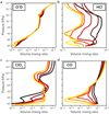 |
Fig. 4 Vertical distribution profiles of the VMRs of O(1D) (a), HCl (b), the ClOX group (c; see also Fig. A.3), and CO (d) displayed in units of mol/mol for the biotic scenarios (see Fig. 1 for the colour legend). |
3.1.3 CH4
The CH4 abundances decrease with increasing solar constant, as shown in Fig. 2c. The surface concentrations fall from 1.46 ppm to 0.57 ppm, 0.22 ppm, 0.11 ppm, 0.06 ppm, and 0.03 ppm for S = 1.0, 1.1, 1.2, 1.3, 1.4, and 1.5, respectively. Larger H2O abundances lead to an increase in OH by more than two orders of magnitude in the lower and middle atmosphere (Fig. A.1), which combines with the increasing rate of CH4 photolysis in the upper layers to increase the overall rate of CH4 oxidation in the atmosphere, effectively increasing the abundances of methane’s main oxidation products CO2 and H2O throughout the atmospheric column. Chlorine atom (Cl) abundances increase to maximum values of 5.43, 42.65, 68.11 pptv in the troposphere for S = 1.3, 1.4, and 1.5, respectively, compared to the 0.001–0.1 pptv abundances seen for S = 1.0–1.2 (Fig. A.3) as already discussed. The additional Cl atoms greatly increase the rate of CH4 ‘s chemical breakdown closer to the surface, resulting in the substantially larger decreases in the CH4 column for S = 1.3–1.5 (Fig. 2c) scenarios.
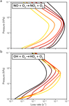 |
Fig. 5 Photochemical loss rate coefficients in the biotic scenarios for the gas-phase removal of O3 with NO (upper panel) and OH (lower panel) for all biotic model scenarios. The reciprocal of the quantity shown gives the atmospheric lifetime in seconds against destruction of O3 by the given reaction (see Fig. 1 for the colour legend). |
3.1.4 N2O
The N2O abundances rather surprisingly increase in the upper (P < 10 hPa) atmosphere as the solar constant increases from the S=1.0 to 1.3 scenarios (Fig. 2). This behaviour is unexpected because increasing instellation is an important photolytic sink for N2O, as is the case for S = 1.4 and 1.5, whereby the N2O abundances over all altitudes decrease to values below those at S = 1.0. The chemical budget of N2O in our model is dominated by (1) biological emission at the surface (held constant in all scenarios), (2) eddy mixing throughout the atmospheric column, which controls the rate of transport of (biomass) N2O from the lower levels up to the middle atmosphere, where it is destroyed in situ, (3) gas-phase removal via photolysis in the UV-B or/and reaction with electronically excited oxygen atoms mainly in the middle atmosphere and above, and (4) minor (<1%) in situ abiotic, gas-phase sources. Further analysis suggested that the N2O mesosphere increase for the S=1.0 to 1.3 scenarios was related to a modest decrease in electronically excited singlet oxygen atoms (O(1D)), which are a sink for N2O. This, in turn arose due to less O3 (a photolytic source for O(1D)) related to HOX destruction in the enhanced steam atmosphere at pressures of 10−3–10−2 hPa, and more H2O, which reacts with O(1D) to produce two OH molecules. Cl atoms also act as a chemical sink for N2O. For S < 1.3, the Cl atom abundances in the troposphere stay below 0.1 pptv and have negligible impact on this biosig-nature. With the increasing rate of HCl photolysis for S ≥ 1.3, the Cl abundances range from 1–100 pptv and take over as the primary atmospheric sink for N2O in the troposphere. This additional chemical sink explains the change in tendency for N2O as the VMRs begin to fall below those calculated at S = 1.0 in the lower atmosphere, but initially increase when pressures are below 1 hPa.
3.2 Response of CO2, hydrogen, and nitrogen reservoirs
3.2.1 CO2 and HOX
Figure 3 presents the VMR profiles of carbon dioxide (CO2), the odd-hydrogen group (HOX = H + OH + HO2; see also Fig. A.1), the odd-nitrogen group (NOX = N + NO + NO2 + NO3; see also Fig. A.2), and nitric acid (HNO3), an important reservoir species for HOX and NOX. With an increasing solar constant and a constant surface flux (Table 1), CO2 VMRs increase from 310.0 ppm at S = 1.0 to 3368.4 ppm at S = 1.4 while maintaining an iso-profile vertical structure (suggesting that chemical timescales are longer than those of transport), but begin to fall at S = 1.5 to a value of 3064.0 ppm. With increasing proximity to the Sun, the UV photolysis of CO2 to CO and O(3P) or O(1D) atoms rises throughout the atmosphere. This is accompanied by an increasing abundance of HOX species produced from the increasing H2O abundances seen in Fig. 1b being produced by the rising rate of photolysis for H2O. The atmospheric production of CO2 is dominated by the catalytic recycling of CO by the hydroxyl radical (OH; Yung & DeMore 1998), which becomes more powerful with the growing HOX abundances as solar constant values rise. This increasing production strength exceeds that of the increasing photolysis of CO2, resulting in CO2 increasing in abundance with increasing S. For S = 1.5 however, this effect reverses, since the increased photolysis rate of CO2 now exceeds the rising rate of CO-OH recombination.
Figure A.1 displays the VMRs of the individual species family members H, OH, and HO2 to the HOX vertical distribution profile. The total HOX concentrations, where pressures exceed 100 hPa (Earth’s tropopause), increases with rising solar constant up to but not including S = 1 .3. These increases are due to the additional OH being introduced by both enhanced H2O VMRs as well as increasing UV fluxes. For S ≥ 1.3, however, the rising UV flux notably increases the abundance of Cl atoms close to the surface through the photolytic breakdown of HCl (see Fig. A.3a). The higher Cl abundances lead to the removal of low-altitude HO2 that replenishes HCl and O2 faster than they can be produced by the breakdown of the additional atmospheric H2O. The increasing UV-C flux (Fig. 1e), a product of the strong decrease in tropospheric O3 (Fig. 2b, described in greater detail in Sect. 3.3.2), also decreases the stability of HO2 near the surface due to an increase in its rate of photolysis. HO2 is the dominant HOX species at pressures greater than 102 hPa and the HOX profiles of Fig. 3 therefore show a decrease close to the surface with increasing S. For atmospheric pressures between 10−1 and 102 hPa, OH becomes the primary species in the HOX family. As it is the direct product of H2O reactions with O(1D) atoms and photolysis the model runs feature enhancements in mid-altitude OH abundances as expected, increasing from VMRs of approximately 0.1 pptv at S = 1.0 to 100 pptv at S = 1.5. This explains the steady rise in the overal HOX group in the middle atmosphere.
At high altitudes (pressures < 0.1 hPa), H atoms are the primary constituent of HOX related to the high rates of UV induced photolysis at the top of the model atmosphere. Between 0.01 and 1 hPa in Fig. A.1, however, the H atom abundances do not vary substantially with increasing solar constant. The O2 VMRs vary between 0.20 and 0.35 mol/mol (Fig. 2a) and provide H atoms with a roughly steady chemical sink as they react to produce HO2. The stability of this chemical sink balances the increasing production of H atoms from the elevating H2O abundances between 0.01 and 1 hPa, resulting in the approximately invariant HOX profile here across S = 1.0–1.5. At higher altitudes up to the model lid (10−4 hPa), the photolysis of H2O and subsequent production of H atoms grows larger than the O2 sink can balance, producing an enhanced H atom abundance with increasing solar constant.
3.2.2 NOX and its reservoirs
The NOX species (Fig. 3c) exhibit three different trends in the lower (P ≥ 100 hPa), middle (100 > P ≥ 0.01 hPa), and upper (P < 0.01 hPa) atmosphere. In the lower atmosphere, NOX abundances increase with increasing solar constant. A fixed surface flux of N2O, coupled with an increasing surface flux of UV radiation, increases the rate of NO production via N2O photolysis in the troposphere. Additionally, a decreasing HO2 abundance close to the surface at high S lowers the chemical sink strength for NO, which is the most abundant NOX family member in the lower atmosphere, and its increasing production and decreasing sink result in an increase in the NOX VMR profile. In the middle atmosphere, NOX abundances fall with an elevating solar constant by between 1 and 2 orders of magnitude. This is related to the conversely increasing HOX (Fig. 3b).
In the mesosphere, the rising photolysis rate of N2 with increasing solar constant leads to an enhancement in the abundance of N atoms, which quickly convert to NOX species. The resulting NO2 molecules are converted to HNO3 by the enhanced HOX abundances, resulting in a decrease in NOX for an increasing S value until the photolytic frequencies of S = 1 .4 and 1.5 are large enough to make N atoms the dominant NOX compound. When this occurs, the NOX concentration becomes roughly invariant above altitudes where pressures are less than 10−3 hPa.
3.3 Response of O(1D), chlorine chemistry, and CO
The VMR profile of O(1D) is presented in Fig. 4a. At pressures greater than 100 hPa, the concentrations decrease by two orders of magnitude with increasing solar constant. Between 1 and 100 hPa, the concentrations remain approximately stable as the solar constant rises. In the region between ≈0.01 and 0.1 hPa the O(1 D) abundances again experience drops from maximum VMRs of 0.27 pptv at S = 1.0 to 3.44×10⁻³ pptv at S = 1.5. At the top of the atmosphere, where pressures are below 10−3 hPa, the concentrations remain stable. The principle source of O(1 D) is the UV photolysis of O3 within the UV-C wavelength range.
CO2 photolysis also provides a source of O(1D), but is less efficient due to its smaller cross-sectional area within the UV-C band. The most efficient sink for O(1D) is collision induced de-excitation with N2, converting O(1D) to O(3P). N2 remains the primary component of the atmosphere (0.78 mol/mol at S = 1.0 and falling to 0.41 mol/mol at S = 1.5). In general, the behaviour of O(1 D) follows the behaviour of O3, detailed in Sect. 3.1.2.
The source of chlorine in all model runs is the surface flux (62.38 Tg yr−1) and volcanic fluxes of HCl (4.30 Tg yr−1) and the surface flux of CH3Cl (2.95 Tg yr−1). The primary sinks of HCl are reactions with OH, and UV photolysis with cross-section maxima centred on 150-160 nm within the UV-C radiation range (Fig. 1e). At pressures greater than 100 hPa, HCl concentrations remain quite stable for instellations of S = 1.0–1.2. UV-C fluxes fall between S = 1.0 and 1.2, whereas OH gradually increases. This results in HCl maintaining concentrations of 0.50–0.60 ppbv for runs at S = 1.0, 1.1, and 1.2. Through S = 1.3–1. 5, the emerging UV-C window near to the surface and the still increasing OH concentration, increase the rate of HCl destruction and its concentration decreases from 0.35 ppbv to 0.12 ppbv. At pressures less than 100 hPa, HCl tends to decrease in abundance gradually with increasing S. Increasing OH concentrations and rising UV fluxes increase the rate of HCl destruction, but the rise in HO2 enables HCl to be reproduced through reactions with Cl atoms, which mitigates the decrease in atmospheric HCl.
Figure 4c presents the ClOX (= Cl + ClO + ClO2) profiles of the various scenarios (see also Fig. A.3). The primary source of ClOX is the photolysis of HCl, to produce Cl atoms, and reactions of HCl with OH to produce ClO. ClO2 is then produced by the three-body reaction of Cl with O2. Figure A.3 presents the individual profiles of the ClOX group members. At pressures greater than 100 hPa OH dominates HCl loss between S = 1.0 and 1.3, resulting in ClO being the dominant member of the ClOX group with concentrations of 0.1–100 pptv (Cl = 10−4–100 pptv). When the UV-C window appears at S = 1.4–1.5, photolysis dominates HCl loss and atomic Cl becomes the main component of ClOX with abundances of 1–10 pptv.
3.4 Comparisons to planet scenarios with no active biosphere
In addition to the six biotic scenarios shown in Table 1, we performed simulations across the same range of instellations with only volcanic outgassing fluxes as input. These scenarios represent an Earth-like planet without any biological emissions at the surface. The surface relative humidity for all scenarios was again fixed to 80%, with layers below the cold trap set to the Manabe– Wetherald profile Manabe & Wetherald (1967) and layers above calculated via photochemistry and diffusion. This is to simulate the presence of an ocean. For simplicity, the negative surface flux of CO2 in Table 1 is tuned to produce a surface CO2 abundance approximately equal to the S = 1.0 biotic value (~310 ppm). A lower negative surface flux would be expected due to an abiotic surface having no land vegetation for photosynthesis and a lack of a biologically driven carbonate-silicate cycle in the oceans, but true consideration of these processes is beyond the scope of the present study. This important caveat is expanded upon in Sect. 4.
Figure 6 presents vertical profiles of the atmospheric temperature and important atmospheric species of the abiotic planet simulations performed by the 1D-TERRA climate-chemistry model compared to the biotic runs. In Fig. 6a, the abiotic temperature profiles (dashed lines) from S = 1.0–1.3 do not produce the temperature inversion between 0.1 and 1 hPa seen in the biotic simulations (solid lines) due to the weakened ozone layer. Surface temperatures reach 280.90 K, 293.86 K, 308.50 K, 332.51 K, 346.94 K, and 364.38 K for S = 1.0–1.5. For S ≥ 1.4, the classical greenhouse effect produced by the rising tropo-spheric water content (Fig. 6b) results in the cold trap rising in altitude as atmospheric temperatures increase. At this point, the water vapour within the troposphere diffuses to the higher altitudes and becomes more comparable in both vertical and column abundance to the biotic simulations below 10 hPa. The cooling of the stratosphere that occurs in the biotic scenarios is not seen in the abiotic scenarios, producing strong temperature differences between biotic and abiotic runs across S = 1.0–1.3 at altitudes with pressures greater than 0.1 hPa.
The lower stratospheric H2O in the abiotic scenarios that arises due to a lower CH4 surface flux is less efficient at trapping the heat travelling upwards, enabling the stratosphere to gradually heat. Without an efficient O3 layer (Fig. 6d) absorbing UV radiation, photolysis rates of H2O in the stratosphere and mesosphere are greater in the abiotic scenarios. At altitudes where pressures range from 10−2–10 hPa, the biotic scenario H2O chemical lifetime ranges between 1 and 10 years. In the abiotic scenarios, these values fall to 0.01–0.1 years due to the greater photolysis rates. The combination of a lower photochemical source in CH4, an increased photochemical sink, and the continued suppression of H2O diffusion from within the troposphere due to the cold trap cause our abiotic scenarios to produce very low mesospheric H2O abundances.
Without the biotic emission of O2 at the surface (Table 1), the abiotic runs produce O2 via atmospheric chemistry only. CO2 photolyses into oxygen atoms, which are capable of combining into molecular O2. As the instellation increases, we see the surface VMRs rise from 1–10 pptv (Fig. 6c), significantly lower than the biotic runs. As O3 is dependent on the O2 abundances, it is produced at levels up to 6 orders of magnitude lower than the biotic counterparts (Fig. 6d). The O3 layer (abundances between 0.01 and 1 ppbv) in the abiotic runs is maintained by the same balance between NOX and HOX groups seen in the biotic runs (Fig. 5) up to and including instellations of S = 1 . 3 . At S = 1.4, the HOX concentrations become three orders of magnitude greater in this pressure region in the abiotic runs than the biotic runs. This increases the sink rate of O3 , resulting in the abiotic O3 layer collapsing from ppbv abundances to 10–2−10−1 pptv abundances.
There are three to four orders of magnitude less methane (Fig. 6e) than their biotic counterparts in the abiotic simulations between instellations S = 1.0 and 1.3 due to the removal of the biomass emissions. The lower CH4 abundances result in a lower photochemical production of H2O above the troposphere. By S = 1.4 vertical diffusion from the troposphere dominates as the source of stratospheric and mesospheric H2O resulting in their differences between the biotic scenario decreasing. As a result, the temperature profiles of the biotic and abiotic simulations become comparable below the troposphere for runs where S ≥ 1.4 (Fig. 6a).
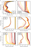 |
Fig. 6 Profiles produced by 1D-TERRA for planets with (solid lines) and without (dashed lines) Earth’s biomass emissions at the surface. The dashed lines represent the abiotic runs. Line colours have the same meanings as in Figs. 1–5 and denote the increasing solar instellation. |
3.5 Emission spectra responses of biosignatures to increasing stellar instellation
Figure 7 presents the resulting emission profiles of the six planet scenarios driven with and without Earth’s biomass surface fluxes. This model takes as input converged temperature, pressure and composition profiles from the 1D-TERRA model and molecular absorption features from the HITRAN line-byline database (Gordon et al. 2022). The spectral resolving power is set to R = 100.
From 5.0–7.1 µm the H2O absorption band dominates the emission spectra in both biotic and abiotic scenarios. With increasing instellation, the increasing H2O abundances in the lower atmosphere dominate the spectral features of the biotic scenarios and their abiotic counterparts. The significantly stronger CH4 and O2 abundances in the biotic runs (Figs. 6c and d) produce marginally stronger absorption features at 6.0–6.5 µm. The first noticeable difference between the biotic and abiotic emission spectra is seen at 7.8–8.0 µm for cases S = 1.0–1.2. These are produced by the presence of larger CH4 and N2O abundances in the biotic cases – as seen in Figs. 6c and f, the abundances in the biotic scenarios fall to negligible concentrations for S > 1.2.
Between 9.0 and 10.0 µm, the O3 layer produced by the biotic surface fluxes of O2 are distinguishable throughout all cases of S . As the O3 abundances in abiotic scenarios are typically 4–6 orders of magnitude lower than their biotic counterparts, the feature on this wavelength range remains as a strong distinguishing signature of biological surface activity. The O3 signature located at 9.6 µm in Fig. 7 remains apparent for runs with instellations up to and including a value of 1.4 – a distance corresponding to 0.85 AU to the Sun. At S = 1.5, the O3 profiles begin to recede in the middle atmosphere (Fig. 2b) and the tropospheric content has fallen to magnitudes under 1 ppbv, which results in the CO2 absorption feature in this wavelength range smearing out that of O3. A similar effect is seen for the O3 feature found at 13.8–14.8 µm. It remains apparent in the GARLIC spectra up to and including runs at S = 1.5, but becomes weakened by the competing CO2 absorption band across this wavelength interval.
From 10.0–13.0 µm, the differences in the atmospheric temperature profiles of biotic and abiotic runs (Fig. 6a) begin to make an impact on the spectra. Approximately 99% of the atmospheric column is contained at pressures above 10 hPa, causing this altitude region to dominate the contributions to the emission spectra. The greater H2O abundances in the stratosphere in biotic cases across S ≤ 1.3, an oxidation product of the biotic CH4 surface fluxes that the abiotic cases lack, produces biotic-abiotic temperature profile differences at pressures > 101 hPa that result in greater emission fluxes across 10–13.0 µm. At the collapse of the cold trap (S ≥ 1.4), the H2O abundances below 100 hPa become approximately equal in the biotic and abiotic scenarios, resulting in temperature profiles that are harder to distinguish, and the differences in their emission features at 10–13.0 µm begin to fall.
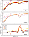 |
Fig. 7 Emission spectra of the six planetary instellation scenarios produced by the GARLIC radiative transfer model. The spectra are produced using a spectral resolving power of R = 100 across a wavelength range of 5.0–20.0 µm. (a) Scenarios with Earth biomass emissions at the surface. (b) Scenarios without Earth biomass emissions at the surface. (c) Difference between the biotic and abiotic scenario fluxes at each respective instellation. |
3.6 Detectability of biomarkers with LIFEsim
LIFEsim, developed by Dannert et al. (2022) and used across works such as Quanz et al. (2022), Konrad et al. (2022), and Alei et al. (2022), was used here to add astrophysical noise signals to the emission spectra produced by the GARLIC radiative transfer code. The absolute difference in received flux from the biotic and abiotic scenarios at each instellation is found at each wavelength interval, and divided by the biotic spectra’s noise level. These calculations are performed over a stellar distance grid of 5–30 pc in intervals of 5 pc, and for LIFE observation times of 24, 48, 120, and 240 hours using the ‘baseline’ scenario. This uses a mirror diameter of 2.0 m, system throughput of 5%, quantum efficiency of 70%, and a spectral resolving power of R = 50. Figure 8 presents the resulting statistical significance of the emission features of this work’s biotic scenarios compared to their corresponding abiotic scenarios. The angular separation of each planet with varying stellar instellation (a, converted from AU to pc) at each system distance (d, in pc) is calculated via tan1 (a/d) and used as LIFEsim input.
Water features in the IR (5.0–7.1 µm; Fig. 7) are indistinguishable between the biotic and abiotic scenarios. Likewise, the CH4 band at 7.7 µm from the biotic runs is not strong enough to produce a feature with statistical significance greater than 0.1 with respect to the abiotic planet spectra for any integration time considered. Increasing the aperture diameter of LIFE to 3.5 m (LIFEsim’s ‘optimistic’ setting; Fig. B.1) and increasing the system throughput and quantum efficiency to a more optimistic 20% and 80%, respectively, enables the statistical significance of the 7.7µm CH4 feature to exceed 0.5 for systems within 7.5 pc for integration times above 120 hours, and ~12.5 pc for 240 hours.
From Fig. 8, the most distinguishable features between biotic and abiotic scenarios are the O3 band found at 9.6 µm and the CO2 (and thermal emission) band at ~15.0 µm. For O3 at 9.6 µm, biotic O3 signals from Earth-size planets within the habitable zone (0.95–1.37 AU, as parameterised by Kasting 1988) only become statistically differentiable (liberally defined here as ≥1.0) from abiotic Earth-like planets for integration time exceeding 120 hours for systems within 12.5 pc when LIFEsim’s baseline scenario was used. The optimistic aperture diameter enables statistical significance of the 9.6 µm to exceed 1.0 for systems 15–20 pc from Earth for integration times above 120 hours (Fig. B.1).
Across 14.0–16.0 µm, the thermal emission band overlaps the CO2 absorption band. As the biotic and abiotic runs hold approximately equal CO2 concentrations, the differences in this region are produced by the differing temperature profiles (Fig. 6a) that also induce temperature broadening of the CO2 bands in the biotic. The ability to distinguish biotic and abiotic runs with instellations S >1.4 is hindered due to the collapse in the cold trap and the rush of H2O into the stratosphere in both the biotic and abiotic scenarios (Fig. 6b). With LIFEsim’s baseline scenario, the thermal profile differences produce emission spectra statistical significances greater than 0.5 for planets within 12.5 pc after 48 hours of observation. Increasing the integration time to 120 and 240 hours raises this distances to 15–20 pc for planets with S = 1.0–1.5. Within the habitable zone (S ≤ 1.1), values of 1.0 can be reached for stars within 12.5 pc after 120 hours.
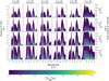 |
Fig. 8 Statistical significance (as a function of wavelength) of the difference in retrieved emission flux calculated via LIFEsim between the biotic and abiotic scenarios studied in this work. The columns (from left to right) show increasing planet instellation; the different rows show different observation integration times (from 24–240 hours). |
4 Discussion
This modelling study does not account for changes to CO2 induced by an active carbonate-silicate cycle, a vital regulator of atmospheric temperature for Earth’s climate. With increasing surface temperatures, the weathering rate of silicate rocks will increase (West et al. 2005) and draws more gaseous CO2 from the atmosphere effectively increasing the CO2 surface sink with increasing instellation. Despite this omission, our biotic scenario with 10% more instellation produces a surface temperature of 304.41 K. This corroborates the prior findings of Caldeira & Kasting (1992) who used a climate model with biologically mediated silicate weathering to study Earth’s biosphere as the Sun’s luminosity rises who modelled a surface temperature of 305 K at S = 1.1. Ozaki & Reinhard (2021) developed a combined biogeochemistry and climate model of Earth’s biosphere to forward-model the atmospheric responses through time. They found that in approximately 1 Gyr, when S ≃1.1, atmospheric O2 may drop below 1% of the present atmospheric level. With the expected decreasing CO2 abundances, the productivity of O2 generating biotic activity becomes limited, which would suppress the current surface flux of O2 with time and increasing solar constant. The surface fluxes of O2 and CO2 are therefore unrealistic for a future-Earth for S > 1.1. Similarly, photosyn-thetic activity for Earth biosystems has optimum temperatures for gross primary productivity that peak between 293 and 308 K and experiences sharp downward trends beyond 313 K (Bennett et al. 2021).
A major result of our work is that ozone could survive warm, damp (hence high HOX) conditions towards the IHZ due to mutual destruction of its catalytic sinks (HOX by NOX). Previous works in literature regarding the study of steam atmosphere climates neglect O3 in the atmosphere, owing to the increased presence of destructive HOX species expected to appear in atmospheres dominated by water vapour (Kasting 1988; Abe & Matsui 1988; Lebrun et al. 2013; Katyal et al. 2019). Similarly, with increasing proximity to the host star the increasing UV-B fluxes would be assumed to further contribute to the photolytic degradation of any ozone layer within the atmosphere. In our work, the presence of a biosphere producing fluxes corresponding to the modern Earth (Table 1) is found to maintain the O3 layer centred on the atmospheric pressure range of 100 – 101 hPa despite the HOX concentrations increasing by more than an order of magnitude due to enhanced water via ocean evaporation. As HOX species react with NOX species to form HOX-NOX reservoir molecules such as HNO2 and HNO3, the weaker influence of NOX as a sink for O3 helps maintain the ozone layer for our simulated Earth-like planets in the IHZ. This could have important consequences for the atmospheric modelling of steam atmospheres, as climate-only simulations could be underestimating the O3 content of the middle atmosphere. As a consequence, climate-chemistry coupled models of steam atmospheres that include a robust C-H-O-N chemistry scheme should be investigated.
Theoretical spectra suggest that the O3 spectral features produced in biotic simulations remain apparent in all instellation scenarios studied. The sharp fall in tropospheric O3 is also shown to open a window to UV-C radiation at S ≥ 1.3, which is capable of stimulating ClOX chemistry close to the surface. As Cl and ClO are strong reducing agents, their impacts on atmospheric chemistry, especially ozone, close to the surface require further work in future photochemical modelling studies of planets close to or beyond the IHZ. We also show that despite the abiotic and biotic abundances differing substantially for Earth-like planets (Fig. 6d), the resulting emission spectra signals are difficult to differentiate from those originating from biologically inactive surfaces. To be a reliable biomarker, extend observation times of greater than 5–10 days should be pursued for Earth-like planets within the habitable zone with LIFE.
Although CH4 is difficult to detect in the infrared emission spectra for planets producing Earth-like surface fluxes, its presence can be inferred indirectly by looking at thermal emission features. For an ‘optimistic’ aperture diameter of 3.5 m, LIFE would be able to detect the greenhouse heating of the atmosphere induced by the H2O produced by CH4 oxidation for systems within 20 pc of our Solar System after viewing periods of 5–10 days. The occurrence rate of Earth-like planets orbiting G-type stars with instellations exceeding 1.0, as estimated by Kopparapu et al. (2018), has baseline estimates ranging from 0.21–0.67. A total of 141 G-type stars have been observed within 20 pc (Gaia Collaboration 2016, 2023) of our Solar System. Applying these Earth occurrence rates to this number of G-type stars, 29–94 Earth-like planets could be available for these measurements to target in future missions.
Our modelling study produces substantially different results to the work of Wolf & Toon (2015), who used a 3D climate model to assess the impacts on Earth’s climate with increasing stellar instellation up to a value of S = 1.21. They calculate global mean temperatures of approximately 360 K at S = 1.21 – at S = 1.2 in our study, surface temperatures only reach 318.93 K (Table 2) and 308.06 K in our biotic and abiotic scenarios, respectively. These differences arise due differences in our water columns; Wolf & Toon (2015) find a global mean column of ~2500 kg m−2 at S = 1.21, compared to ~250 kg m−2 in our simulations at S = 1.2. When our model water column reaches ~2125 kg m−2 at S = 1.5 in our biotic scenarios, the greenhouse effect (calculated as the difference between the surface outbound longwave radiation and the top of atmosphere outbound longwave radiation) are comparable to Wolf & Toon (2015). These water column differences arise from the differences of the 3D and 1D models used. Wolf & Toon (2015) computes changing water vapour via 3D advection processes, turbulent mixing in the troposphere, and condensation and evaporation. The results presented here, in the 1D approach, simply force the tropospheric water content to the Manabe–Wetherald profile with a fixed surface relative humidity of 80%, and calculate stratospheric and mesospheric H2O via vertical diffusion and photochemical calculations. Neglecting photochemical production and loss of H2O in the stratosphere and mesosphere also led climate studies such as Wolf & Toon (2015) to underestimate the atmospheric water content of modern Earth, which will lead to discrepancies appearing between their work and studies such as ours that incorporate atmospheric photochemistry.
Solar constants studied in this work for the six biotic model scenarios, with corresponding distances to the Sun, the resultant amount of H2O at the model surface in percentage by volume and partial pressure, and the surface temperature.
5 Conclusions
Using 1D-TERRA to study the atmospheric composition of a planet hosting an Earth-like biosphere as solar instellation progressively increases has revealed the following key features:
For the biotic runs, the atmospheric O2 content increases up to solar instellations of S = 1.2 (≃1603 W m−2) due to, for example, catalytic recycling of HOX into O2. The increasing rate of H2O and CO2 photolysis also enables additional abiotic O2 to form faster than the increasing UV photolysis of O2. Above S = 1.2, however, the ClOX in the troposphere engages in photochemical loss cycles with O2, which causes abundances to start falling;
The stratospheric O3 layer, centred between 100 and 101 hPa, is maintained above parts-per-million magnitudes up to and including runs with instellations of S = 1.5 (≃2042 W m−2). This is counter to our initial hypothesis and the assumptions of prior climate models of water-rich atmospheres. With four orders of magnitude more H2O than at S = 1 .0, the increasing HOX concentrations coupled with the increasing flux of UV (175.0–405.0 nm) radiation was expected to efficiently destroy the O3 layer. Instead, the increasing concentration of O2 from abiotic atmospheric chemistry and the suppression of ozone’s NOX sink from reactions with HOX balance the increasing chemical and photolytic sinks;
Biogenic CH4 becomes unidentifiable in emission spectra after solar instellations of S = 1 .2. The elevated HOX and UV radiation fluxes greatly increase the rate of photochemical loss, and beyond S = 1 .3 the elevated ClOX in the troposphere induces chemical loss rates that push CH4 to abundances below 0.1 pptv at atmospheric pressures below 102 hPa;
UV-C radiation fluxes decrease with increasing solar instellation due to the increasing atmospheric H2O content up to and including values of S = 1.2 (≃1633 W m−2 total flux at the top of the atmosphere). Above S = 1.2, the tropospheric ozone abundances plummet due to enhanced ClOX loss processes initiated by the enhanced photolysis of outgassed HCl;
The ozone band at 9.6 µm will require observation times greater than 120 hours for systems within 10 pc to reliably be designated a biosignature on an Earth-like planet if LIFE uses an aperture diameter of 2.0 m. Extending the aperture diameter to 3.5 m will enable the inference to be made for systems within 20 pc;
Thermal emission features between 14.0 and 16.0 µm in atmospheres with biological surface fluxes within 0.88 AU of their host stars are strong biomarkers, indicating the presence of strong CH4 modern-Earth-like surface emissions. Beyond 0.85 AU, the collapse of the abiotic scenarios’ cold trap makes the abiotic and biotic thermal emission fluxes more difficult to distinguish.
Appendix A Additional volume mixing ratio profiles
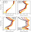 |
Fig. A.1 Individual VMRs of H (a), OH (b), and HO2 (c) that summed together produce the profile of the HOX chemical group (Figure 3b), as well as H2O2 (d), a reservoir for HOX species, for biotic model runs at solar constant 1.0, 1.1, 1.2, 1.3, 1.4, and 1.5 (see Figure 1 for the colour legend). |
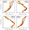 |
Fig. A.2 Individual VMRs of NO (a), NO2 (b), and NO3 (c) that summed together produce the profile of the NOX chemical group (d; Figure 3c) for biotic model runs at solar constant 1.0, 1.1, 1.2, 1.3, 1.4, and 1.5 (see Figure 1 for the colour legend). |
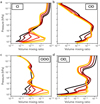 |
Fig. A.3 Individual VMRs of Cl (a), ClO (b), and ClOO (c) that summed together produce the profile of the ClOX chemical group (d; Figure 4c) for biotic model runs at solar constant 1.0, 1.1, 1.2, 1.3, 1.4, and 1.5 (see Figure 1 for the colour legend). |
Appendix B Additional statistical significance study
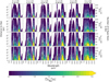 |
Fig. B.1 Same as Figure 8, but for LIFEsim’s ‘optimistic’ setting which assumes an aperture diameter of 3.5m, R = 50, quantum efficiency = 80%, and throughput = 15%. |
References
- Abe, Y., & Matsui, T. 1985, JGR: Solid Earth, 90, C545 [Google Scholar]
- Abe, Y., & Matsui, T. 1988, J. Atmos. Sci., 45, 3081 [NASA ADS] [CrossRef] [Google Scholar]
- Alei, E., Konrad, B. S., Angerhausen, D., et al. 2022, A&A, 665, A106 [NASA ADS] [CrossRef] [EDP Sciences] [Google Scholar]
- Bennett, A. C., Arndt, S. K., Bennett, L. T., et al. 2021, Glob. Change Biol., 27, 4727 [NASA ADS] [CrossRef] [Google Scholar]
- Caldeira, K., & Kasting, J. F. 1992, Nature, 360, 721 [NASA ADS] [CrossRef] [Google Scholar]
- Catling, D. C., & Kasting, J. F. 2017, Atmospheric Evolution on Inhabited and Lifeless Worlds (Cambridge University Press) [CrossRef] [Google Scholar]
- Chameides, W. L., Stedman, D. H., Dickerson, R. R., Rusch, D. W., & Cicerone, R. J. 1977, J. Atmos. Sci., 34, 143 [NASA ADS] [CrossRef] [Google Scholar]
- Dannert, F. A., Ottiger, M., Quanz, S. P., et al. 2022, A&A, 664, A22 [NASA ADS] [CrossRef] [EDP Sciences] [Google Scholar]
- Dorn, C., & Lichtenberg, T. 2021, ApJ, 922, L4 [NASA ADS] [CrossRef] [Google Scholar]
- Elkins-Tanton, L. T. 2008, EPSL, 271, 181 [NASA ADS] [CrossRef] [Google Scholar]
- Elkins-Tanton, L. T. 2012, Annu. Rev. Earth Pl. Sci., 40, 113 [NASA ADS] [CrossRef] [Google Scholar]
- Etiope, G., & Ciccioli, P. 2009, Science, 323, 478 [NASA ADS] [CrossRef] [Google Scholar]
- Gaia Collaboration (Prusti, T., et al.) 2016, A&A, 595, A1 [NASA ADS] [CrossRef] [EDP Sciences] [Google Scholar]
- Gaia Collaboration (Vallenari, A., et al.) 2023, A&A, 674, A1 [NASA ADS] [CrossRef] [EDP Sciences] [Google Scholar]
- Gaillard, F., Bernadou, F., Roskosz, M., et al. 2022, EPSL, 577, 117255 [NASA ADS] [CrossRef] [Google Scholar]
- Gao, P., Hu, R., Robinson, T. D., Li, C., & Yung, Y. L. 2015, ApJ, 806, 249 [NASA ADS] [CrossRef] [Google Scholar]
- Garvin, J. B., Getty, S. A., Arney, G. N., et al. 2022, PSJ, 3, 117 [NASA ADS] [Google Scholar]
- Gebauer, S., Grenfell, J., Lehmann, R., & Rauer, H. 2018, Astrobiology, 18, 856 [NASA ADS] [CrossRef] [Google Scholar]
- Ghail, R., Wilson, C. F., & Widemann, T. 2016, in AAS/Division for Planetary Sciences Meeting Abstracts, 48, 216 [Google Scholar]
- Gierasch, P. J., & Conrath, B. J. 1985, in Recent Advances in Planetary Meteorology, ed. G. E. Hunt, 121 [Google Scholar]
- Giorgi, F., & Chameides, W. 1985, JGR: Atmos., 90, 7872 [NASA ADS] [CrossRef] [Google Scholar]
- Gordon, I. E., Rothman, L. S., Hargreaves, R. J., et al. 2022, J. Quant. Spec. Radiat. Transf., 277, 107949 [NASA ADS] [CrossRef] [Google Scholar]
- Grenfell, J. L., Stracke, B., von Paris, P., et al. 2007, P&SS, 55, 661 [NASA ADS] [CrossRef] [Google Scholar]
- Haqq-Misra, J., Kopparapu, R. K., Batalha, N. E., Harman, C. E., & Kasting, J. F. 2016, ApJ, 827, 120 [NASA ADS] [CrossRef] [Google Scholar]
- Harman, C. E., Kopparapu, R. K., Stefánsson, G., et al. 2022, PSJ, 3, 45 [NASA ADS] [Google Scholar]
- Höning, D., Baumeister, P., Grenfell, J. L., Tosi, N., & Way, M. J. 2021, JGR: Planets, 126, e2021JE006895 [CrossRef] [Google Scholar]
- Kasting, J. F. 1988, Icarus, 74, 472 [NASA ADS] [CrossRef] [Google Scholar]
- Kasting, J. F. 1993, Science, 259, 920 [NASA ADS] [CrossRef] [Google Scholar]
- Katyal, N., Nikolaou, A., Godolt, M., et al. 2019, ApJ, 875, 31 [NASA ADS] [CrossRef] [Google Scholar]
- Katyal, N., Ortenzi, G., Grenfell, J. L., et al. 2020, A&A, 643, A81 [NASA ADS] [CrossRef] [EDP Sciences] [Google Scholar]
- Khalil, M., & Rasmussen, R. 1984, Atmos. Environ., 18, 1805 [NASA ADS] [CrossRef] [Google Scholar]
- Kite, E. S., & Schaefer, L. 2021, ApJ, 909, L22 [NASA ADS] [CrossRef] [Google Scholar]
- Kitzmann, D., Patzer, A. B. C., von Paris, P., Godolt, M., & Rauer, H. 2011, A&A, 534, A63 [NASA ADS] [CrossRef] [EDP Sciences] [Google Scholar]
- Konrad, B., Alei, E., Quanz, S., et al. 2022, A&A, 664, A23 [NASA ADS] [CrossRef] [EDP Sciences] [Google Scholar]
- Kopparapu, R. K., Hébrard, E., Belikov, R., et al. 2018, ApJ, 856, 122 [NASA ADS] [CrossRef] [Google Scholar]
- Lammer, H., Zerkle, A. L., Gebauer, S., et al. 2018, A&AR, 26, 1 [CrossRef] [Google Scholar]
- Lebrun, T., Massol, H., Chassefière, E., et al. 2013, JGR: Planets, 118, 1155 [NASA ADS] [CrossRef] [Google Scholar]
- Lichtenegger, H. I. M., Kislyakova, K. G., Odert, P., et al. 2016, JGR: Space Phys., 121, 4718 [NASA ADS] [CrossRef] [Google Scholar]
- Manabe, S., & Wetherald, R. T. 1967, J. Atmos. Sci, 24, 241 [NASA ADS] [CrossRef] [Google Scholar]
- Marcq, E., Salvador, A., Massol, H., & Davaille, A. 2017, JGR: Planets, 122, 1539 [NASA ADS] [CrossRef] [Google Scholar]
- Meadows, V. S. 2017, Astrobiology, 17, 1022 [CrossRef] [Google Scholar]
- Nikolaou, A., Katyal, N., Tosi, N., et al. 2019, ApJ, 875, 11 [Google Scholar]
- O’Rourke, J. G., Wilson, C. F., Borrelli, M. E., et al. 2023, Space Sci. Rev., 219, 10 [CrossRef] [Google Scholar]
- Ostberg, C., Kane, S. R., Li, Z., et al. 2023, AJ, 165, 168 [NASA ADS] [CrossRef] [Google Scholar]
- Ozaki, K., & Reinhard, C. T. 2021, Nat. Geosci., 14, 138 [NASA ADS] [CrossRef] [Google Scholar]
- Pyle, D., & Mather, T. 2009, Chem. Geol., 263, 110 [CrossRef] [Google Scholar]
- Quanz, S. P., Ottiger, M., Fontanet, E., et al. 2022, A&A, 664, A21 [NASA ADS] [CrossRef] [EDP Sciences] [Google Scholar]
- Ricker, G. R., Latham, D., Vanderspek, R., et al. 2010, in American Astronomical Society Meeting Abstracts, 215, 450 [Google Scholar]
- Rugheimer, S., & Kaltenegger, L. 2018, ApJ, 854, 19 [NASA ADS] [CrossRef] [Google Scholar]
- Salvador, A., Avice, G., Breuer, D., et al. 2023, Space Sci. Rev., 219, 51 [NASA ADS] [CrossRef] [Google Scholar]
- Sander, R. 2015, Atmos. Chem. Phys., 15, 4399 [CrossRef] [Google Scholar]
- Scheucher, M., Wunderlich, F., Grenfell, J. L., et al. 2020, ApJ, 898, 44 [Google Scholar]
- Schreier, F., Gimeno García, S., Hedelt, P., et al. 2014, J. Quant. Spec. Radiat. Transf., 137, 29 [NASA ADS] [CrossRef] [Google Scholar]
- Schreier, F., Gimeno García, S., Vasquez, M., & Xu, J. 2015, JQSRT, 164, 147 [NASA ADS] [CrossRef] [Google Scholar]
- Schreier, F., Milz, M., Buehler, S., & von Clarmann, T. 2018a, JQSRT, 211, 64 [NASA ADS] [CrossRef] [Google Scholar]
- Schreier, F., Städt, S., Hedelt, P., & Godolt, M. 2018b, MolAst. 11, 1 [NASA ADS] [Google Scholar]
- Schreier, F., Gimeno García, S., Hochstaffl, P., & Städt, S. 2019, Atmosphere, 10, 262 [NASA ADS] [CrossRef] [Google Scholar]
- Segura, A., Kasting, J. F., Meadows, V., et al. 2005, Astrobiology, 5, 706 [Google Scholar]
- Smrekar, S. E., Dyar, D., Helbert, J., et al. 2020, in EPSC, EPSC2020-447 [Google Scholar]
- Sossi, P. A., Burnham, A. D., Badro, J., et al. 2020, Sci. Adv., 6, eabd1387 [NASA ADS] [CrossRef] [Google Scholar]
- Sossi, P. A., Tollan, P. M., Badro, J., & Bower, D. J. 2023, EPSL, 601, 117894 [NASA ADS] [CrossRef] [Google Scholar]
- Turbet, M., Bolmont, E., Chaverot, G., et al. 2021, Nature, 598, 276 [CrossRef] [Google Scholar]
- Way, M. J., & Del Genio, A. D. 2020, JGR: Planets, 125, e2019JE006276 [CrossRef] [Google Scholar]
- Way, M. J., & Genio, A. D. D. 2020, JGR: Planets, 125, e2019JE006276 [CrossRef] [Google Scholar]
- West, A. J., Galy, A., & Bickle, M. 2005, EPSL, 235, 211 [NASA ADS] [CrossRef] [Google Scholar]
- Westall, F., Höning, D., Avice, G., et al. 2023, Space Sci. Rev., 219, 17 [NASA ADS] [CrossRef] [Google Scholar]
- Widemann, T., Smrekar, S. E., Garvin, J. B., et al. 2023, Space Sci. Rev., 219, 56 [NASA ADS] [CrossRef] [Google Scholar]
- Wolf, E., & Toon, O. 2015, JGR: Atmos., 120, 5775 [NASA ADS] [CrossRef] [Google Scholar]
- Wunderlich, F., Scheucher, M., Godolt, M., et al. 2020, ApJ, 901, 126 [Google Scholar]
- Yung, Y. L., & DeMore, W. B. 1998, Photochemistry of Planetary Atmospheres (New York, NY: Oxford University Press) [Google Scholar]
- Zahnle, K., Schaefer, L., & Fegley, B. 2010, Cold Spring Harb. Persp. Bio., 2, a004895 [Google Scholar]
All Tables
Biomass surface fluxes, dry deposition velocities, and volcanic outgassing fluxes for trace gas species used in all model runs in this work.
Solar constants studied in this work for the six biotic model scenarios, with corresponding distances to the Sun, the resultant amount of H2O at the model surface in percentage by volume and partial pressure, and the surface temperature.
All Figures
|
Fig. 1 Temperature (a), H2O vapour volume mixing ratio in mol/mol (b), and the UV-A (c), UV-B (d), UV-C (e), and FUV (f) fluxes calculated by 1D-TERRA for a (biotic) Earth-like planet with the mean incoming instellation increased from 1.0 (modern Earth) up by a factor of 1.5 (orbiting a Sun-like star at 0.82 AU). |
| In the text | |
|
Fig. 2 Vertical distribution profiles of the VMRs of O2 (a), O3 (b), CH4 (c), and N2O (d) displayed in units of mol/mol for the biotic scenarios (see Fig. 1 for the colour legend). |
| In the text | |
|
Fig. 3 Vertical distribution profiles of the VMRs of CO2 (a), the HOX group (b; see also Fig. A.1), the NOX group (c; see also Fig. A.2), and HNO3 (d) displayed in units of mol/mol for the biotic scenarios (see Fig. 1 for the colour legend). |
| In the text | |
|
Fig. 4 Vertical distribution profiles of the VMRs of O(1D) (a), HCl (b), the ClOX group (c; see also Fig. A.3), and CO (d) displayed in units of mol/mol for the biotic scenarios (see Fig. 1 for the colour legend). |
| In the text | |
|
Fig. 5 Photochemical loss rate coefficients in the biotic scenarios for the gas-phase removal of O3 with NO (upper panel) and OH (lower panel) for all biotic model scenarios. The reciprocal of the quantity shown gives the atmospheric lifetime in seconds against destruction of O3 by the given reaction (see Fig. 1 for the colour legend). |
| In the text | |
|
Fig. 6 Profiles produced by 1D-TERRA for planets with (solid lines) and without (dashed lines) Earth’s biomass emissions at the surface. The dashed lines represent the abiotic runs. Line colours have the same meanings as in Figs. 1–5 and denote the increasing solar instellation. |
| In the text | |
|
Fig. 7 Emission spectra of the six planetary instellation scenarios produced by the GARLIC radiative transfer model. The spectra are produced using a spectral resolving power of R = 100 across a wavelength range of 5.0–20.0 µm. (a) Scenarios with Earth biomass emissions at the surface. (b) Scenarios without Earth biomass emissions at the surface. (c) Difference between the biotic and abiotic scenario fluxes at each respective instellation. |
| In the text | |
|
Fig. 8 Statistical significance (as a function of wavelength) of the difference in retrieved emission flux calculated via LIFEsim between the biotic and abiotic scenarios studied in this work. The columns (from left to right) show increasing planet instellation; the different rows show different observation integration times (from 24–240 hours). |
| In the text | |
|
Fig. A.1 Individual VMRs of H (a), OH (b), and HO2 (c) that summed together produce the profile of the HOX chemical group (Figure 3b), as well as H2O2 (d), a reservoir for HOX species, for biotic model runs at solar constant 1.0, 1.1, 1.2, 1.3, 1.4, and 1.5 (see Figure 1 for the colour legend). |
| In the text | |
|
Fig. A.2 Individual VMRs of NO (a), NO2 (b), and NO3 (c) that summed together produce the profile of the NOX chemical group (d; Figure 3c) for biotic model runs at solar constant 1.0, 1.1, 1.2, 1.3, 1.4, and 1.5 (see Figure 1 for the colour legend). |
| In the text | |
|
Fig. A.3 Individual VMRs of Cl (a), ClO (b), and ClOO (c) that summed together produce the profile of the ClOX chemical group (d; Figure 4c) for biotic model runs at solar constant 1.0, 1.1, 1.2, 1.3, 1.4, and 1.5 (see Figure 1 for the colour legend). |
| In the text | |
|
Fig. B.1 Same as Figure 8, but for LIFEsim’s ‘optimistic’ setting which assumes an aperture diameter of 3.5m, R = 50, quantum efficiency = 80%, and throughput = 15%. |
| In the text | |
Current usage metrics show cumulative count of Article Views (full-text article views including HTML views, PDF and ePub downloads, according to the available data) and Abstracts Views on Vision4Press platform.
Data correspond to usage on the plateform after 2015. The current usage metrics is available 48-96 hours after online publication and is updated daily on week days.
Initial download of the metrics may take a while.