| Issue |
A&A
Volume 692, December 2024
|
|
|---|---|---|
| Article Number | A31 | |
| Number of page(s) | 10 | |
| Section | Astronomical instrumentation | |
| DOI | https://doi.org/10.1051/0004-6361/202449158 | |
| Published online | 29 November 2024 | |
Diffuse radio sky models using large-scale shapelets
ASTRON, Netherlands Institute for Radio Astronomy,
Oude Hoogeveensedijk 4,
7991 PD
Dwingeloo,
The Netherlands
★ Corresponding author; This email address is being protected from spambots. You need JavaScript enabled to view it.
Received:
4
January
2024
Accepted:
23
October
2024
Abstract
Aims. Sky models used in radio interferometric data-processing primarily consist of compact and discrete radio sources. When there is a need to model large-scale diffuse structure such as the Galaxy, specialized source models are sought after for the sake of simplicity and computational efficiency. We propose the use of shapelet basis functions for modeling the large-scale diffuse structure in various radio interferometric data-processing pipelines.
Methods. The conventional source model construction using shapelet basis functions is restricted to using images of smaller size due to limitations in computational resources such as memory. We propose a novel shapelet decomposition method to lift this restriction, enabling the use of images of millions of pixels (as well as a wide spectral bandwidth) for building models of large-scale diffuse structure. Furthermore, the application of direction-dependent errors onto diffuse sky models is an expensive operation that is often performed as a convolution. We propose using some specific properties of shapelet basis functions to apply these direction-dependent errors as a product of the model coefficients, which avoids the need for convolution.
Results. We provide results based on simulations and real observations. In order to measure the efficacy of our proposed method in modeling large-scale diffuse structure, we considered the direction-dependent calibration of simulated as well as real LOFAR observations that have a significant number of diffuse large-scale structure. The results show that by including large-scale shapelet models of the diffuse sky, we are able to overcome a major problem of existing calibration techniques, which do not model this large-scale diffuse structure, that is, the suppression of this large-scale diffuse structure because the model is incomplete.
Key words: instrumentation: interferometers / methods: numerical / techniques: interferometric
© The Authors 2024
 Open Access article, published by EDP Sciences, under the terms of the Creative Commons Attribution License (https://creativecommons.org/licenses/by/4.0), which permits unrestricted use, distribution, and reproduction in any medium, provided the original work is properly cited.
This article is published in open access under the Subscribe to Open model. This email address is being protected from spambots. You need JavaScript enabled to view it. to support open access publication.
1 Introduction
In addition to compact (extragalactic) radio sources, the low- frequency radio sky is also covered by large-scale diffuse structure, the most obvious of which is the Galaxy (Zheng et al. 2017; Byrne et al. 2021). The effect of this large-scale diffuse structure on high-precision data processing (e.g., for the study of the epoch of reionization (EoR) and cosmic dawn (CD), Mellema et al. 2013; Gehlot et al. 2019; Gehlot et al. 2020) is considered to be an issue that is well worthy a thorough investigation (Gehlot et al. 2021; Jackson & Grobler 2023; Barry et al. 2024). These investigations recommended the inclusion of large-scale diffuse structure in the sky models used in low-frequency interferometric data processing. However, the commonly used data models (e.g., in radio interferometric calibration) only accommodate compact and discrete radio sources, and the inclusion of large-scale structure would incur significant computational cost (Carozzi & Woan 2009). Therefore, the commonly used calibration strategy is to indirectly minimize the effect of large-scale diffuse structure on the calibration performance. For example, short baselines that are mostly affected by large-scale diffuse structure can be excluded while the calibration is performed (Patil et al. 2016, 2017). On the other hand, some form of filtering can be pre-applied to the data to remove the signal caused by large-scale diffuse structure prior to calibration (Charles et al. 2023). These indirect remedies are not always feasible. For instance, when there are not enough long baselines on which the calibration can be based (Munshi et al. 2024) because when short baselines are excluded, many usable constraints are excluded as well (Ewall-Wice et al. 2017).
In this paper, we propose a method for directly modeling the large-scale diffuse structure in low-frequency radio interferometric data using shapelet basis functions (Refregier 2001; Refregier & Bacon 2003). The novelty of the proposed work can be summarized as follows:
Shapelet model construction has so far only used (relatively) small images as input (Yatawatta 2010, 2011; Line et al. 2020). Modern radio interferometers are capable of covering large fields of view, yielding images with sizes of up to millions or billions of pixels (Yatawatta 2014). The use of these large-scale images as input to the shapelet model creation is computationally restricted because it requires a large amount of memory. We overcome this limitation here by using a divide-and-conquer approach: We use the accelerated projection-based consensus (APC) algorithm (Azizan-Ruhi et al. 2019). This not only enables us to work with images with millions of pixels in size (covering a large field of view at high resolution), but also images made at a large number of frequencies covering a wide bandwidth. In other words, we are able to construct both wide-field and wideband shapelet models using a distributed divide-and-conquer approach in a computationally feasible manner.
Interferomety with large fields of view, which is the norm for low-frequency interferometers, inevitably has to encounter systematic errors (e.g., the beam shape) that cover a large field of view. The application of these systematic errors onto diffuse sky models requires convolution in the Fourier space, which is a computationally expensive operation (Lanman et al. 2022). We overcome the use of convolution by exploiting certain properties of the shapelet basis functions (Refregier 2001; Refregier & Bacon 2003), in particular, their orthogonality. By exploiting these properties, we can perform coordinate-free convolutions entirely using coefficient multiplications of the basis functions. This significantly reduces the computational cost.
As an application of large-scale shapelet models in radio interferometry, we extend our previous work on distributed direction-dependent calibration with spectral and spatial regularization (Yatawatta 2015, 2021) to incorporate models of the large-scale diffuse sky.
In calibration, a commonly used alternative to modeling large- scale diffuse structure in the aforementioned manner is to represent this structure by sources with compact support, such as point sources or Gaussians. While this representation scheme is much simpler, it has several drawbacks: (i) A large number of components are needed for an accurate representation of the large-scale diffuse structure (increased computational cost). (ii) The inherent spatial continuity in the diffuse structure is not always guaranteed (less realistic). And finally, (iii) these models are tuned to one specific observation and their reuse in other observations is not straightforward, for example, due to coordinate transformation, projection, and uv-coverage (limited reusability). On the other hand, in image synthesis and deconvolution, a plethora of alternative methods exist that specialize in modeling diffuse structure, (e.g. Cornwell 2008; Bhatnagar & Cornwell 2004; Rich et al. 2008; Rau & Cornwell 2011; Junklewitz et al. 2016), and the integration of these methods into direction-dependent calibration is worth further investigation.
The remaining paper is organized as follows: in Sect. 2 we introduce shapelet basis functions and the data model we used in radio interferometry. We also introduce the application of direction-dependent effects onto shapelet source models as a multiplication of the shapelet coefficients (in the image space, instead of a convolution in Fourier space). In Sect. 3, we provide details of the wide-field and wide-band shapelet model construction using the APC algorithm. In Sect. 4 we provide details of the use of large-scale diffuse sky models in a distributed directiondependent calibration. We provide results based on simulations and real data in Sects. 5 and 6, respectively, to illustrate the use of large-scale shapelet models in a direction-dependent calibration. Finally, we draw our conclusions in Sect. 7.
Notation: Lowercase bold letters refer to column vectors (e.g., y). Uppercase bold letters refer to matrices (e.g., C). Unless otherwise stated, all parameters are complex numbers. The set of integers is given as ℤ, the set of complex numbers is given as ℂ, and the set of real numbers is given as ℝ. The matrix inverse, pseudo-inverse, transpose, and Hermitian transpose are referred to as (·)−1, (·)† ,(·)T, and (·)H, respectively. The matrix Kronecker product is given by ⊗. The identity matrix of size N is given by IN. The Frobenius norm is given by || ⋅ || and the L-1 norm is given by || ⋅ ||1.
2 Data model
In this section, we introduce the (rectangular) shapelet basis functions, the commonly used radio interferometric data model, and our expansion of this model to accommodate a large-scale diffuse structure using shapelet basis functions.
2.1 Shapelet basis functions
We use the rectangular shapelet basis functions (Refregier 2001; Berry et al. 2004; Chang & Refregier 2002; Melchior et al. 2009) as the basis for a sky model construction. One-dimensional shapelets or Gauss-Hermite polynomials can be given as
![Mathematical equation: ${\phi _n}(x,\beta ) = {\left[ {{2^n}\sqrt \pi n!\beta } \right]^{ - {1 \over 2}}}{H_n}\left( {{x \over \beta }} \right)\exp \left( { - 0.5{{\left( {{x \over \beta }} \right)}^2}} \right),$](/articles/aa/full_html/2024/12/aa49158-24/aa49158-24-eq1.png) (1)
(1)
where x (∈ ℝ) is the coordinate, n (ℤ+) is the order of the basis function, and β (∈ ℝ+) is the scale factor. The Hermite polynomial of order n is given by Hn (⋅). In two dimensions (with coordinates x and y), the basis is constructed as a product of one-dimensional basis functions, that is, ϕn (x,y,β) = ϕn (x,β)ϕn (y,β).
Shapelet basis functions are already being used for radio astronomical source modeling in practice (e.g. Yatawatta 2010, 2011; Line et al. 2020). One noteworthy property that we exploit is the fact that the Fourier transform of ϕn(x,β) is jnϕn(u, 1/β), where u is the Fourier dual of x. In other words, given the shapelet decomposition in real (image) space, we can calculate its Fourier transform with linear computational complexity.
We state one additional property of rectangular shapelet basis functions that will be useful later.
Lemma 1. Given functions f (x) and g(x) and their shapelet decompositions, f (x), scale βf, coefficients fn, n = 0,…, Mf −1, g(x), scale βg, coefficients gm, m = 0,…, Mg − 1, the shapelet decomposition of the product h(x) = f (x)g(x) with scale βh and coefficients hl, l = 0,…, Mh − 1 can be given in closed form by (2).
The coefficients of the product are
 (2)
(2)
where Clmn(βh,βf, βg) is given by (Refregier & Bacon 2003)
![Mathematical equation: $\matrix{ {{C_{lmn}}(a,b,c)} \hfill \cr { = v{{\left[ {{{( - 2)}^{l + m + n}}\sqrt \pi l!m!n!abc} \right]}^{ - {1 \over 2}}}{L_{l,m,n}}\left( {\sqrt 2 {v \over a},\sqrt 2 {v \over b},\sqrt 2 {v \over c}} \right),} \hfill \cr } $](/articles/aa/full_html/2024/12/aa49158-24/aa49158-24-eq3.png) (3)
(3)
for even values of l + m + n and  . Furthermore, Ll,m,n(a, b, c) in (3) can be evaluated using L0,0,0(a, b, c) = 1 and the recurrence relations for even values of l + m + n,
 (4)
(4)
and with Ll,m,n (a, b, c) = 0 for odd values of l + m + n.
The proof of Lemma 1 can be found by following the proof given in Bergé et al. (2019). When we are free to select the scale βh and the number of the basis functions Mh of the product, we can set βh to the lower value of βf and βg and Mh to the higher value of Mf and Mg .
The Fourier relation and the results in Lemma 1 directly extend to the two-dimensional basis that is used for modeling large-scale diffuse structure.
2.2 Radio interferometric data model
We consider an interferometric array with N receivers. The output visibilities of the baseline formed by stations p and q can be given as (Hamaker et al. 1996)
 (5)
(5)
where  are the observed data at frequency fi at P distinct frequencies, i ∈ [1, P]. The right-hand side of Eq. (5) describes the model used to predict the visibilities given the sky model. We consider K distinct directions in the sky, each direction being modeled by a set of compact sources, and the coherencies for the k-th direction are given by
  . The systematic errors determined by calibration along the k-th direction are given by
  .
.
The coherencies representing the diffuse sky model are given by the mapping  ) in Eq. (5). The systematic errors
  that are attributed to the diffuse sky model are used as an antenna-based scaling of the diffuse sky model (hence, they are independent of the direction), and the true direction dependence is represented by
  . Therefore, the physical relevance of
  is to account for any discrepancy of the total flux in the diffuse sky model and the true sky, mainly because we do not have zero-length baselines (or baselines close to zero). We consider
  to be a function of two tensors, namely S and Z, with S describing the source model and Z describing the spatial model (e.g., the beam shape and ionosphere). One noteworthy property that is common to both S and to Z is the use of shapelet basis functions whose coefficients are given by S and Z while evaluating
  . The origin of the diffuse sky model (x = y = 0) can in general be anywhere in the sky (this position is used to calculate the phase contribution), but for simplicity, we consider its origin to coincide with the phase center of the observation. Moreover, both S and Z can consist of multiple bases (e.g., with different scales β and number of basis functions M).
Finally, the noise and the effect of unmodeled sources are given by the last term in Eq. (5), that is, Npq (∈ ℂ2×2), which is generally considered to be consisting of elements drawn from a complex circular Gaussian distribution. Given the data model (5), the objective of the calibration is to determine  for all p and k = 0,…, K. We formulated the calibration as a distributed optimization problem in our previous work (Yatawatta 2015, 2021), which we briefly describe here. For brevity, we group all solutions for one direction k and one frequency fi as
![Mathematical equation: ${{\bf{J}}_{k{f_i}}} \buildrel \Delta \over = {\left[ {{\bf{J}}_{1k\,fi}^T,{\bf{J}}_{2k\,{f_i}}^T, \ldots ,{\bf{J}}_{Nk\,{f_i}}^T} \right]^T},$](/articles/aa/full_html/2024/12/aa49158-24/aa49158-24-eq17.png) (6)
(6)
where  groups the N solutions for all stations into one block.
The core principle in spectrally and spatially regularized direction-dependent calibration can be given as
 (7)
(7)
where  is a basis in frequency and Φk (∈ ℂ2G×2) is a basis in space, while Z (∈ ℂ2FN×2G) is the global model that can be used to derive all solutions
  for all k and fi (Yatawatta 2021). The bases can be constructed from any polynomial. For example,
 (8)
(8)
creates a basis in frequency using  , which is a set of F polynomials evaluated at frequency fi and a basis in space using ϕk (∈ ℂG×1), which is a set of G polynomials in space (two dimensional) that are evaluated at the coordinates pointing toward the k-th direction.
The spectral regularization is achieved by enforcing the constraint
 (9)
(9)
and the spatial regularization is achieved by enforcing the constraint
 (10)
(10)
and we describe the constrained calibration in detail in Sect. 4.
The spatial basis functions ϕk are created using the shapelet basis as described in Sect. 2.1. In order to evaluate  for any given baseline p, q and frequency fi, we evaluate the shapelet coefficients (using the appropriate scale factors) for the source model given by coefficients S and the shapelet coefficients for the spatial model given by Z. We then select the coefficients for stations p and q. We note that Eq. (2) describes a scalar product, but the same relation holds when we find a product of coherencies (∈ ℂ2×2). We also note that we need to apply Eq. (2) twice, first to find the product of the (Hermitian) spatial model for station q with the source coherency, and thereafter, to find the product of the spatial model for station p with the result of the previous step. Finally, we use the Fourier equivalence of the shapelet basis functions to calculate the visibilities for
  .
.
Looking back at Eq. (5), we see that the unknowns are not only  given by Eq. (6), but also Z, which in turn is dependent on
  . In other words, there is a hidden cyclic dependence, and this might lead to instability in the calibration. We break this dependence by introducing the constraint
 (11)
(11)
and use  in Eq. (5), where the only unknowns are
  . The spatial model used for predicting the diffuse sky model, that is,
  in Eq. (11) is updated with a delay, as we describe in Sect. 4.
Ideally, when there are no direction-dependent systematic errors, the spatial model should be isotropic, or in other words, the gain should be unity along all directions. We find the isotropic spatial model  as
as
 (12)
(12)
where  , with 1N (∈ ℝN×1) being a vector of all ones. As we describe in Sect. 4, we keep the spatial model used for predicting the diffuse sky model
  as close to
  as possible to improve the stability of calibration. This is mostly due to the fact that Z can be biased in the case of imperfect sky models (for directions k = 1 . . . , K), especially when we start with a small number of directions K. As we progress, we can increase K to cover the full sky, but initially, this is not always possible.
3 Accelerated projection-based consensus
In this section, we describe shapelet model construction using large images, typically over millions of pixels, as input. For the simplest case, we consider an image of size Nx × Ny = NI pixels that is represented by a vector  . Based on this image, we need to construct a model with M basis functions whose coefficients are given by x ∈ ℝM×1. The basis matrix is given by
  , where each row of A is created by the M basis functions evaluated at the pixel coordinates representing the corresponding row of b. The solution for x is found by solving
 (13)
(13)
which is directly solvable when the size of A in Eq. (13) is small. However, we consider the situation where A cannot fit in memory (let alone finding the inverse of A) because either NI or M or both are large. We therefore cannot directly solve Eq. (13) as in the case for building models for compact diffuse sources.
In a more practical situation, we create a family of models (with varying values for scale β and the number of basis functions M) for any given image. In this case, for instance, with d bases, the number of columns in A is increased even further (sum of all M for d bases). Furthermore, we can build a model with a frequency dependence, where b in Eq. (13) is a concatenation of images at different frequencies. In this case, the number of rows of A is increased as well (the bases at each frequency are evaluated with a known frequency dependence).
In these situations, instead of directly solving Eq. (13), we use a divide-and-conquer approach. We divide the original problem into B subproblems as Eq. (14)
![Mathematical equation: $\left[ {\matrix{ {{{\bf{A}}_1}} \cr {{{\bf{A}}_2}} \cr \vdots \cr {{{\bf{A}}_B}} \cr } } \right]{\bf{x}} = \left[ {\matrix{ {{{\bf{b}}_1}} \cr {{{\bf{b}}_2}} \cr \vdots \cr {{{\bf{b}}_B}} \cr } } \right],$](/articles/aa/full_html/2024/12/aa49158-24/aa49158-24-eq42.png) (14)
(14)
where we divided the original matrix A (size NI × M) into submatrices Ai (size ni × M, ni ≈ NI /B) and the original vector b (size NI) into subvectors bi (size ni), i ∈ [1, B]. The summation Σi ni = NI. We apply the accelerated projection-based consensus (APC) algorithm (Azizan-Ruhi et al. 2019) to solve Eq. (14). The pseudo-code for APC is given in Algorithm 1.
Require: Number of subtasks B, momentum factors γ,η ∈ (0,1], and maximum iterations T.
1: Divide A into B submatrices and b into B subvectors by selecting subsets of rows to obtain Ai, bi, i = 1…, B.
2: Find initial solutions,  .
.
3: Find projection matrices  .
.
4: Initialize the global solution  .
.
5: for t = 0,…, T − 1 do
6: Compute agents update in parallel  .
.
7: Fusion center updates  .
.
8: end for
9: Return  as the solution.
By making B large enough, we can break up any large problem such as Eq. (13) into manageable subproblems. The B subtasks in Algorithm 1 can be executed in parallel, which makes this also suitable for a distributed implementation. The most computationally expensive operation is finding the projection matrices Pi at line 3 of Algorithm 1. However, when each Ai is full rank, the projection matrix Pi = 0, and this essentially makes Algorithm 1 a consensus-averaging algorithm. We do not need all Ai s to be full rank. In fact, the reason for having the projection matrices Pi is to handle the case when Ais are not full rank.
When any Ai is not full rank (e.g., when ni < M), we can use the singular-value decomposition (SVD) to reduce the computational cost of the steps given at lines 2 and 3 in Algorithm 1 as listed in Algorithm 2.
 and Pi
Require:  , rank-deficient ni < M, and bi.
1: Find SVD  orthogonal,
  diagonal.
2: Find  by filling its diagonal by the nonzero diagonal terms of Si (at most ni).
3: Find  ,
,
4: Find the projection matrix  , where
  is the reduced identity matrix with only the first ni diagonal elements having 1.
5: Return  and Pi.
It is possible to make B large such that ni = 1 (each submatrix is a row), and even in this case, we can achieve convergence of Algorithm 1, provided that we select the number of iterations, that is, T, large enough. In Sect. 6 we show an application of Algorithm 1.
4 Calibration with diffuse sky models
In this section, we expand a spectrally and spatially constrained direction-dependent calibration to include models for a large- scale diffuse structure. Under the assumption that the noise Npq in Eq. (5) has complex circular Gaussian random variables, the cost function to minimize to obtain the maximum likelihood estimate of  can be given as
 (15)
(15)
where the cost is accumulated over all baselines (which are part of the calibration) and a finite time interval Δt. When the short baselines are excluded during calibration, the summation is made over a subset of all available baselines.
With the additional constraints (9) and (10), the spectrally and spatially regularized calibration is defined as
![Mathematical equation: $\eqalign{ & \left\{ {{{\bf{J}}_{k{f_i}}}, \ldots ,{{\bf{Z}}_k}:\forall k,i} \right\} = \mathop {\arg \min }\limits_{{{\bf{J}}_{k\,{f_i}}}, \ldots ,{{\bf{Z}}_k}} \mathop {\mathop \sum \nolimits^ }\limits_i {g_{{f_i}}}\left( {\left\{ {{{\bf{J}}_{k\,{f_i}}}:\forall k} \right\}} \right) \cr & \,\,\,\,\,\,\,{\rm{subject to}}{{\bf{J}}_{k\,{f_i}}} = {{\bf{B}}_{{f_i}}}{{\bf{Z}}_k},\quad i \in [1,P],k \in [0,K] \cr & {\rm{}}\,\,\,\,\,\,\,\,\,\,\,\,\,\,\,\,\,\,\,\,\,\,\,\,\,\,\,\,\,\,\,\,\,\,\,\,\,\,\,\,\,\,\,\,\,\,\,\,\,{\rm{and}}{{\bf{Z}}_k} = {{{\bf{\bar Z}}}_k},k \in [0,K]. \cr} $](/articles/aa/full_html/2024/12/aa49158-24/aa49158-24-eq60.png) (16)
(16)
In conjunction, the update of the global spectral-spatial model can be defined as
 (17)
(17)
where λ (∈ ℝ+) is the L-2 regularization factor, and µ (∈ ℝ+) is the L-1 regularization factor. Both λ and µ are introduced to keep the global model Z low-energy and sparse. Moreover, the global model used in  is updated independently of Z, but under the constraint that they are equal.
In order to solve Eq. (16), we form the augmented Lagrangian as
 (18)
(18)
where the Lagrange multipliers  and Xk (∈ ℂ2FN×2) are introduced for the spectral and spatial constraints. The regularization factors ρ and α (∈ ℝ+) are chosen for each of these constraints. Moreover, it is also possible to select ρ and α distinctly per each direction k (e.g., as ρk and αk), which is common practice.
Furthermore, in order to solve Eq. (17), we also form the augmented Lagrangian as
 (19)
(19)
where the Lagrange multiplier Ψ (∈ ℂ2FN×2G) and the corresponding regularization factor γ (∈ ℝ+) are used for the constraint (11).
Minimization of both Eqs. (18) and (19) can be achieved as two interleaved iterations of the alternating direction method of multipliers (ADMM) algorithm (Boyd et al. 2011). The essence of the minimization can be summarized as follows:
Solve
 using generic direction-dependent calibration (Kazemi et al. 2011; Kazemi & Yatawatta 2013) to minimize Eq. (18).
Solve Zk by setting gradient of
 ) to zero as in Eq. (20).
Solve for Z and
 by minimizing Eq. (19).
Update the prediction of the diffuse sky model using
 .
.
By repeating the steps 1–4 above, we are able to reach a stable calibration end result as we show using simulations and real data in Sects. 5 and 6.
We elaborate some of the above steps 1–4 in the following text. In step 2, the solution for Zk is obtained in closed form as
 (20)
(20)
In step 3, solving for Z involves a sparsity-constrained minimization. We therefore use the fast iterative shrinkage and thresholding algorithm (FISTA Beck & Teboulle 2009) to find Z. In order to use FISTA, we need to provide the differentiable cost function h(Z),
 (21)
(21)
and the gradient
 (22)
(22)
When we have found Z in Eq. (19), we find  in closed form by finding the gradient of Eq. (19),
 (23)
(23)
and equating it to zero as
 (24)
(24)
The complete calibration algorithm including the diffuse sky model is summarized in Algorithm 3. This algorithm is designed to run on a distributed computer with one fusion center and several compute agents. In this manner, we maximize the parallelism by exploiting the inherent data parallelism of radio interferometers (which collect and store data at multiple frequencies).
Require: A: number of ADMM iterations, C: cadence of the spatial model update, ρ, α,γ: regularization factors.
1: Initialize  to zero ∀k, i.
2: Initialize  using (12).
3: for a = 1,…, A do
4: {Do in parallel ∀k, i at all compute agents and the fusion center}
5: Compute agents to minimize (18) for  .
.
6: Fusion center solves (20) for Zk .
7:  .
.
8: if a is a multiple of C then
9: Fusion center updates Z using (21) and (22).
10: Fusion center updates  using (10).
11:  .
.
12: Fusion center updates  using (24).
13:  .
.
14: Compute agents to update the diffuse sky model prediction  .
.
15: end if
16: end for
 |
Fig. 1 Sample images (Stokes I, not deconvolved, natural weights) made using simulated data, covering about 10 × 10 square degrees in the sky. (a) Image before calibration. (b) Diffuse sky and the weak sources that are hidden in the simulated data. (c) Residual image after calibration, only using spectral regularization. (d) Residual image after calibration with spectral and spatial regularization. (e) Residual image after calibration with spectral and spatial regularization and using the diffuse sky model. Images (b)–(e) have the same intensity scale. |
5 Simulation results
In this section, we present the results to illustrate the efficacy of the proposed Algorithm 3 based on simulated observations. The simulations were made in a Monte Carlo manner, where we randomized the sky model (including the large-scale diffuse structure) as well as the systematic errors in addition to the noise. We simulated the LOFAR highband antenna (HBA) array (van Haarlem et al. 2013), with N = 62 stations observing in the frequency range [115, 185] MHz. The pointing center of the telescope was randomly selected to be either the north celestial pole (NCP) or 3C196. We selected P = 8 channels that uniformly covered the frequency range, and the duration of each observation was kept at 10 min with an integration time of 10 s.
The simulated sky model consisted of K = 20 compact sources that were randomly spread across a 30 × 30 square degree field of view. Their intrinsic flux densities were randomly chosen in the range [1, 10] Jy, and their spectral indices were randomly sampled from a standard normal distribution. An additional 400 weak sources (point sources and Gaussian sources), with flux densities in the range [0.01, 0.5] Jy and a power-law spectral index of −2, were randomly placed in the field of view and were not included in the calibration sky model.
The diffuse sky model was randomly generated as follows. In each simulation, we generated three shapelet models for the Stokes I, Q, and U diffuse emission. In each shapelet model, the model order  was uniformly sampled from [10, 20], and therefore, each shapelet decomposition had M basis functions. The scale of the shapelet basis β was uniformly sampled from the range [0.01, 1], but if this was too high for the field of view, that is,
  , we sampled β from the range
 ![Mathematical equation: $[2,2.001]/\sqrt M $](/articles/aa/full_html/2024/12/aa49158-24/aa49158-24-eq87.png) . Finally, the M shapelet coefficients were randomly sampled from the standard normal distribution. We only used these shapelet models for the simulation of data, and when we calibrated, we perturbed the shapelet models to make them more error prone and realistic (we did not use Algorithm 1 in this section). We perturbed the scale β and the coefficients by 10% of their original value by adding appropriately scaled noise drawn from the standard normal distribution.
. Finally, the M shapelet coefficients were randomly sampled from the standard normal distribution. We only used these shapelet models for the simulation of data, and when we calibrated, we perturbed the shapelet models to make them more error prone and realistic (we did not use Algorithm 1 in this section). We perturbed the scale β and the coefficients by 10% of their original value by adding appropriately scaled noise drawn from the standard normal distribution.
The systematic errors  in Eq. (6) were generated to have specific properties, that is, randomness, smooth variation over time and frequency, and smoothness over space (over k). We first generated 8N random planes in space with a domain equal to the image coordinates. The 8N planes were for each real value of
  . For a selected fi, we filled
  with values drawn from the complex standard normal distribution and added a fraction of the value of the random planes evaluated at the coordinates for the direction k = 0,…, K. Next, we generated 8N third-order random polynomials in frequency and multiplied
  to evaluate the systematic errors for all frequencies. Simultaneously, we generated 8N random sinusoidal polynomials in time and multiplied
  with these polynomials to evolve the systematic errors over time. During the simulation, the systematic errors were used to corrupt the data. In addition, the LOFAR HBA beam model (station beam and dipole beam) were also applied to the data. When we simulated the diffuse shapelet models, we only applied the systematic errors evaluated at the center of the source.
We added noise to the simulated data with a signal-to-noise ratio of 1/0.05. The elements of Npq in Eq. (5) were drawn from a complex standard normal distribution.
During the spectrally and spatially regularized calibration, we used a Bernstein polynomial basis with F = 3 terms for  and a shapelet basis with G = 4 terms for ϕk in Eq. (8). The scale of the shapelet basis was determined automatically depending on the spread of the K directions given in the sky model. We evaluated three calibration settings:
Calibration with only a spectral regularization.
Calibration with both a spectral and spatial regularization.
Calibration with both a spectral and spatial regularization with a diffuse sky model.
The regularization factors ρk and αk in Eq. (18) were determined as follows. We set ρk proportional to the flux density of the k-th source, with the maximum value of ρk being limited to 200. We set αk inversely proportional to the distance of the k-th source from the pointing center. We limited the maximum value of αk to 1. When the diffuse foreground model was also included in the calibration, we set ρ = 1, α = 0.1 and γ = 0.1 for this direction (in addition, λ = µ = 1 e − 3). The number of ADMM iterations was set to A = 50, and the cadence of the spatial model update was set to C = 3.
The calibration was repeated for every 10 time samples, or in other words, for every 10 × 10 = 100 s. We did not exclude the short baselines during the calibration. Therefore, all baselines were used to evaluate Eq. (15). When the solutions  were found, the residual was calculated as
 (25)
(25)
We did not subtract the diffuse sky model in Eq. (25), and it should remain in the residual.
We made images of the residual data using natural weights to enhance the large-scale structure (if any). One such example is shown in Fig. 1. In addition to showing the data and residual images, we also show the image in which we only simulated the diffuse model in Fig. 1b. The residual image obtained after calibration with a diffuse sky model in Fig. 1e clearly agrees well with the diffuse model. In contrast, Figs. 1c and d show a much greater suppression of the diffuse model, which is the main reason we need to remedy this issue, for example, by excluding short baselines from the calibration.
We performed 40 Monte Carlo simulations, and we provide some results in Fig. 2. To evaluate the simulations quantitatively, we provide two metrics. First, we measured the variance (calculated using the whole image) of images similar to those shown in Fig. 1. We expect the variance in the residual to decrease because we subtracted most of the signal to calculate the residual (25). However, we should not expect the noise variance to go too low, which would indicate some overfitting. The number of constraints compared to the degrees of freedom we used is more or less on the border of becoming ill-constrained for our calibration setup, and this is reflected in a noise reduction below a value that is realistic. As shown in Fig. 2a, the noise variance of the residual images for the calibration without the diffuse sky model is generally lower than the variance of the residual images that were calibrated with a diffuse sky model.
A second metric is a measure of the diffuse foreground power that remains in the residual. In order to measure this, we found the correlation factor between the image of the diffuse foreground (e.g., Fig. 1b) and the residual image. A higher correlation indicates lower suppression of the diffuse foreground in the residual image. Since we worked with data in full polarization, we found the correlation factor of Stokes I images, Stokes Q images, and Stokes U images separately and found the mean absolute value of the correlation. In Fig. 2b, we compare the correlation for each of the calibration settings. Once again, a calibration without a diffuse sky model leads to a significant suppression of the diffuse foreground, while a diffuse sky model (even an approximate one) remedies this issue.
 |
Fig. 2 Results of 40 simulations. (a) Variance in the images made before and after calibration. Three calibration scenarios are shown, where the calibration without a diffuse sky model gives lower noise, probably due to overfitting. (b) Correlation of the diffuse foreground with the residual. When the diffuse sky model is included in the calibration, much of the diffuse sky model is preserved. However, in other calibration scenarios, the diffuse sky is significantly suppressed (this is the reason for excluding short baselines in these calibration scenarios). |
6 Real observations
In this section, we provide an example based on real data that includes substantial diffuse emission. We considered an observation of the Galactic plane (centered on the supernova remnant G46.08–0.3) using the LOFAR HBA array. We used 100 subbands in the frequency range [124, 148] MHz. Each subband had a bandwidth of 0.192 MHz. We used a 4-hour duration of data that were acquired by project LC4_010 in July 2015 (Polderman 2021) and are now public at the LOFAR long-term archive.
The image after direction-independent calibration and averaging all 100 subbands is shown in Fig. 3a. None of the images shown was deconvolved (i.e., dirty images). This image shows a field of view of about 10 × 10 square degrees using 18 000 × 18 000 pixels of size 2″.
For a direction-dependent calibration, we built a sky model of about 100 compact point sources and four shapelet models to represent the compact diffuse structure using the data that made the image in Fig. 3a. In addition, we created one shapelet model for the large-scale diffuse background using Algorithm 1 as described in Sect. 3 (the total number of pixels NI was over 300 million, requiring its use here). In Fig. 4, we show the full sky model (simulated at a single frequency at 137 MHz) as well as the model for the large-scale diffuse structure. The shapelet models are not 100% accurate, as seen by comparing Figs. 3 and 4. We intentionally kept this discrepancy to enhance the effect that is due to model error. Moreover, the image in Fig. 3a shows more compact sources than what is included in our model shown in Fig. 4a. We only included about one-third of all the visible point sources in the sky model, and this was also to test our algorithm under less favorable circumstances.
We grouped the sky model into 30 source clusters (K = 30) for a direction-dependent calibration with a solution time interval of 5 min. We considered three calibration scenarios:
Calibration without the large-scale diffuse sky model and using all baselines (excluding autocorrelations). Spectral regularization with F = 3.
Calibration without the large-scale diffuse sky model, but excluding baselines shorter than 300 wavelengths from calibration. Spectral regularization with F = 3. The residual was calculated for all baselines.
Calibration with a large-scale diffuse sky model (Algorithm 3) and using all baselines, excluding autocorrelations. Spectral and spatial regularization with F = 3, G = 4, and γ= 0.1.
After calibration, we subtracted all compact sources from the sky model to calculate the residual (25), and the residual image obtained for scenario 3 above is shown in Fig. 3b. In order to study the performance of the above three scenarios in a quantitative manner, we show zoomed in versions of the residual images in Figs. 5b–d together with the image before the directiondependent calibration in Fig. 5a. Furthermore, in Fig. 6 we show the difference images, that is, the image after the calibration was subtracted from the image before calibration.
Visually, the images in Figs. 5b–d look similar, but we are interested in the quantitative differences. In order to do this, we selected a small area in these images without compact sources but with diffuse structure (shown by the red square). We evaluated the total flux within this square before and after calibration for all three aforementioned calibration schemes. We recovered about 50% of the flux in calibration scenario 1, where all baselines were included in the calibration. By excluding baselines shorter than 300 wavelengths, we recovered 104% of the flux, which is an increase that is not physically possible. When a model for the large-scale diffuse structure was included, we recovered 88% of the flux even when we included all baselines in the calibration. This also agrees with the results obtained using simulated data in Sect. 5 (see Fig. 2a). Moreover, the difference images in Fig. 6 qualitatively show the suppression of diffuse structure due to calibration using all baselines without a model for the diffuse structure.
The increase in recovered flux when the short baselines were excluded from the calibration needs an explanation. In order to do this, we show the gridded visibility data (real part of Stokes I) in Fig. 7. We only show the gridded visibilities within a radius of 600 wavelengths in Fig. 7. In Fig. 7a, the gridded data before calibration are shown, and in Figs. 7b–d, the gridded data after calibration are shown for the three calibration scenarios.
The differences in Figs. 7b–d are not entirely obvious. In order to highlight the differences, if any, we subtracted the gridded visibilities after calibration with all baselines (i.e., Fig. 7b) from all other gridded visibilities, as shown in Fig. 8. Fig. 8a primarily shows the sky model dominated by compact sources that are subtracted to find the residual in Eq. (25). A subtler effect is seen in Fig. 8b, which is the difference between a calibration including all baselines and a calibration excluding baselines shorter than 300 wavelengths. A disk clearly appears with a radius equal to 300 wavelengths in Fig. 8b. This is due to the statistical leverage (Patil et al. 2016). This leverage effect artificially boosts the residual visibilities within the 300 wavelength radius, which explains the flux increase in Fig. 5c. The inclusion of a diffuse sky model and using all baselines in calibration does not suffer from this effect, as shown in Fig. 8c.
Based on the results in this section, we conclude that the inclusion of a model for the large-scale diffuse structure during the calibration minimizes the suppression of this large-scale structure. The exclusion of short baselines can also minimize this suppression, but it suffers from statistical leverage that artificially boosts the short-baseline signals.
 |
Fig. 3 Images (a) before and (b) after direction-dependent calibration at 137 MHz after averaging all images made by 100 subbands. The images were not deconvolved and have a size of 18 000 × 18 000 pixels with a 2″ pixel size. The units of the color bar are in Jy/PSF. |
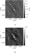 |
Fig. 4 Sky model simulated for a single subband at 137 MHz. The image size is 18 000 × 18 000 pixels with a 2″ pixel size. The full sky model is shown in (a), and the large-scale diffuse sky model is shown in (b). The shapelet model used in (b) has M = 400 basis functions. The color-bar units are in Jy/PSF, but we note the difference in the color-bar limits in (a) and (b). |
 |
Fig. 5 Zoomed-in image covering about 4 × 4 square degrees (a) before calibration, (b) calibration with all baselines, (c) calibration excluding baselines shorter than 300 wavelengths, and (d) calibration without excluding short baselines and with a model for the large-scale diffuse structure. The rectangle in red is about 500 × 500 pixels, and within this rectangle, the sum of all pixels is (a) 1105, (b) 597, (c) 1154, and (d) 977 Jy/PSF, respectively. |
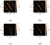 |
Fig. 6 Full-field images with 18 000 × 18 000 pixels with a size of 2″ × 2″. The image before calibration is shown in (a). The difference images, that is, the image before calibration minus the image after calibration, are shown in (b), (c), and (d) for various calibration schemes: (b) calibration with all baselines, (c) calibration excluding baselines shorter than 300 wavelengths, and (d) calibration without excluding short baselines and with a model for the large-scale diffuse structure. Because we subtracted a sky model consisting of only compact sources during calibration, the difference images in a perfect calibration should also show what is being subtracted: the compact sources and their artifacts. However, as we see in (b), we also subtracted or suppressed a significant fraction of the diffuse structure when we included all baselines in the calibration. This suppression is much lower in both (c) and (d). |
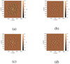 |
Fig. 7 Gridded visibility data (Stokes I, real part) covering a disk with a radius of 600 wavelengths (a) before calibration, (b) calibration with all baselines, (c) calibration excluding baselines shorter than 300 wavelengths, and (d) calibration with all baselines and with a model for the large-scale diffuse structure. |
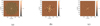 |
Fig. 8 Difference in the gridded visibilities, where the gridded visibilities of the data after calibration using all baselines were subtracted from the gridded visibilities in all other scenarios (a) data before calibration, (b) calibration excluding baselines shorter than 300 wavelengths, and (c) calibration including all baselines and with a model for the large-scale diffuse structure. An inner disk with a radius of 300 wavelengths is clearly visible in (b), indicating an artificial increase in the values of this gridded visibilities within this disk. |
7 Conclusions
We have proposed methods for building and including large- scale diffuse sky models in the processing of radio interferometric data using shapelet basis functions. The simulations and results based on real data showed that this method minimizes the suppression of large-scale diffuse structure in the data during a direction-dependent calibration, without incurring significant computational cost. Therefore, this method will enable the inclusion of short baselines in the calibration, which increases the number of usable constraints and improves the end result.
Future work on this topic will focus on adapting the proposed techniques to basis functions other than shapelets as well as using the APC algorithm in other areas in radio interferometric data-processing, such as in image deconvolution.
Acknowledgements
We thank I. Polderman, M. Haverkorn and Marco Iaco- belli for providing us the LOFAR data used in Section 6 and for assisting with accessing the LOFAR archive. We thank the editor and reviewer for valuable comments. LOFAR, the Low Frequency Array designed and constructed by ASTRON, has facilities in several countries, owned by various parties (each with their own funding sources), and collectively operated by the International LOFAR Telescope (ILT) foundation under a joint scientific policy. The following software already implement the algorithms described in this paper: SAGECAL (https://sagecal.sourceforge.net/), SHAPELET- GUI (https://github.com/SarodYatawatta/shapeletGUI), and EXCON IMAGER (https://sourceforge.net/projects/exconimager/).
References
- Azizan-Ruhi, N., Lahouti, F., Avestimehr, A. S., & Hassibi, B. 2019, IEEE Trans. Sig. Proc., 67, 3806 [CrossRef] [Google Scholar]
- Barry, N., Line, J. L. B., Lynch, C. R., Kriele, M., & Cook, J. 2024, ApJ, 964, 158 [NASA ADS] [CrossRef] [Google Scholar]
- Beck, A., & Teboulle, M. 2009, SIAM J. Imaging Sci., 2, 183 [CrossRef] [Google Scholar]
- Bergé, J., Massey, R., Baghi, Q., & Touboul, P. 2019, MNRAS, 486, 544 [CrossRef] [Google Scholar]
- Berry, R., Hobson, M., & Withington, S. 2004, MNRAS, 354, 42 [Google Scholar]
- Bhatnagar, S., & Cornwell, T. J. 2004, A&A, 426, 747 [NASA ADS] [CrossRef] [EDP Sciences] [Google Scholar]
- Boyd, S., Parikh, N., Chu, E., Peleato, B., & Eckstein, J. 2011, Found. Trends®Mach. Learn., 3, 1 [Google Scholar]
- Byrne, R., Morales, M. F., Hazelton, B., et al. 2021, MNRAS, 510, 2011 [NASA ADS] [CrossRef] [Google Scholar]
- Carozzi, T. D., & Woan, G. 2009, MNRAS, 395, 1558 [NASA ADS] [CrossRef] [Google Scholar]
- Chang, T.-C., & Refregier, A. 2002, ApJ, 354, 42 [Google Scholar]
- Charles, N., Kern, N., Bernardi, G., et al. 2023, MNRAS, 522, 1009 [CrossRef] [Google Scholar]
- Cornwell, T. J. 2008, IEEE J. sel. Top. Sig. Proc., 2, 793 [NASA ADS] [CrossRef] [Google Scholar]
- Ewall-Wice, A., Dillon, J. S., Liu, A., & Hewitt, J. 2017, MNRAS, 470, 1849 [CrossRef] [Google Scholar]
- Gehlot, B. K., Mertens, F. G., Koopmans, L. V. E., et al. 2019, MNRAS, 488, 4271 [Google Scholar]
- Gehlot, B. K., Mertens, F. G., Koopmans, L. V. E., et al. 2020, MNRAS, 499, 4158 [NASA ADS] [CrossRef] [Google Scholar]
- Gehlot, B. K., Jacobs, D. C., Bowman, J. D., et al. 2021, MNRAS, 506, 4578 [NASA ADS] [CrossRef] [Google Scholar]
- Hamaker, J. P., Bregman, J. D., & Sault, R. J. 1996, A&AS, 117, 137 [NASA ADS] [CrossRef] [EDP Sciences] [Google Scholar]
- Jackson, J. P., & Grobler, T. L. 2023, MNRAS, 525, 3740 [CrossRef] [Google Scholar]
- Junklewitz, H., Bell, M. R., Selig, M., & Enßlin, T. A. 2016, A&A, 586, A76 [NASA ADS] [CrossRef] [EDP Sciences] [Google Scholar]
- Kazemi, S., & Yatawatta, S. 2013, MNRAS, 435, 597 [NASA ADS] [CrossRef] [Google Scholar]
- Kazemi, S., Yatawatta, S., Zaroubi, S., et al. 2011, MNRAS, 414, 1656 [Google Scholar]
- Lanman, A. E., Murray, S. G., & Jacobs, D. C. 2022, ApJS, 259, 22 [NASA ADS] [CrossRef] [Google Scholar]
- Line, J. L. B., Mitchell, D. A., Pindor, B., et al. 2020, PASA, 37, e027 [NASA ADS] [CrossRef] [Google Scholar]
- Melchior, P., Andrae, R., Maturi, M., & Bartelmann, M. 2009, A&A, 493, 727 [NASA ADS] [CrossRef] [EDP Sciences] [Google Scholar]
- Mellema, G., Koopmans, L. V. E., Abdalla, F. A., et al. 2013, Exp. Astron., 36, 235 [NASA ADS] [CrossRef] [Google Scholar]
- Munshi, S., Mertens, F. G., Koopmans, L. V. E., et al. 2024, A&A, 681, A62 [NASA ADS] [CrossRef] [EDP Sciences] [Google Scholar]
- Patil, A. H., Yatawatta, S., Zaroubi, S., et al. 2016, MNRAS, 463, 4317 [NASA ADS] [CrossRef] [Google Scholar]
- Patil, A. H., Yatawatta, S., Koopmans, L. V. E., et al. 2017, ApJ, 838, 65 [NASA ADS] [CrossRef] [Google Scholar]
- Polderman, I. 2021, PhD thesis, Radboud University, The Netherlands [Google Scholar]
- Rau, U., & Cornwell, T. J. 2011, A&A, 532, A71 [NASA ADS] [CrossRef] [EDP Sciences] [Google Scholar]
- Refregier, A. 2001, MNRAS, 000, 42 [Google Scholar]
- Refregier, A., & Bacon, D. 2003, MNRAS, 338, 48 [NASA ADS] [CrossRef] [Google Scholar]
- Rich, J. W., de Blok, W. J. G., Cornwell, T. J., et al. 2008, AJ, 136, 2897 [NASA ADS] [CrossRef] [Google Scholar]
- van Haarlem, M. P., Wise, M. W., Gunst, A. W., et al. 2013, A&A, 556, A2 [NASA ADS] [CrossRef] [EDP Sciences] [Google Scholar]
- Yatawatta, S. 2010, in 2010 IEEE Sensor Array and Multichannel Signal Processing Workshop, 69 [Google Scholar]
- Yatawatta, S. 2011, in 2011 XXXth URSI General Assembly and Scientific Symposium, 1 [Google Scholar]
- Yatawatta, S. 2014, in 2014 XXXIth URSI General Assembly and Scientific Symposium (URSI GASS, 1 [Google Scholar]
- Yatawatta, S. 2015, MNRAS, 449, 4506 [Google Scholar]
- Yatawatta, S. 2021, MNRAS, 510, 2718 [Google Scholar]
- Zheng, H., Tegmark, M., Dillon, J. S., et al. 2017, MNRAS, 464, 3486 [NASA ADS] [CrossRef] [Google Scholar]
All Figures
|
Fig. 1 Sample images (Stokes I, not deconvolved, natural weights) made using simulated data, covering about 10 × 10 square degrees in the sky. (a) Image before calibration. (b) Diffuse sky and the weak sources that are hidden in the simulated data. (c) Residual image after calibration, only using spectral regularization. (d) Residual image after calibration with spectral and spatial regularization. (e) Residual image after calibration with spectral and spatial regularization and using the diffuse sky model. Images (b)–(e) have the same intensity scale. |
| In the text | |
|
Fig. 2 Results of 40 simulations. (a) Variance in the images made before and after calibration. Three calibration scenarios are shown, where the calibration without a diffuse sky model gives lower noise, probably due to overfitting. (b) Correlation of the diffuse foreground with the residual. When the diffuse sky model is included in the calibration, much of the diffuse sky model is preserved. However, in other calibration scenarios, the diffuse sky is significantly suppressed (this is the reason for excluding short baselines in these calibration scenarios). |
| In the text | |
|
Fig. 3 Images (a) before and (b) after direction-dependent calibration at 137 MHz after averaging all images made by 100 subbands. The images were not deconvolved and have a size of 18 000 × 18 000 pixels with a 2″ pixel size. The units of the color bar are in Jy/PSF. |
| In the text | |
|
Fig. 4 Sky model simulated for a single subband at 137 MHz. The image size is 18 000 × 18 000 pixels with a 2″ pixel size. The full sky model is shown in (a), and the large-scale diffuse sky model is shown in (b). The shapelet model used in (b) has M = 400 basis functions. The color-bar units are in Jy/PSF, but we note the difference in the color-bar limits in (a) and (b). |
| In the text | |
|
Fig. 5 Zoomed-in image covering about 4 × 4 square degrees (a) before calibration, (b) calibration with all baselines, (c) calibration excluding baselines shorter than 300 wavelengths, and (d) calibration without excluding short baselines and with a model for the large-scale diffuse structure. The rectangle in red is about 500 × 500 pixels, and within this rectangle, the sum of all pixels is (a) 1105, (b) 597, (c) 1154, and (d) 977 Jy/PSF, respectively. |
| In the text | |
|
Fig. 6 Full-field images with 18 000 × 18 000 pixels with a size of 2″ × 2″. The image before calibration is shown in (a). The difference images, that is, the image before calibration minus the image after calibration, are shown in (b), (c), and (d) for various calibration schemes: (b) calibration with all baselines, (c) calibration excluding baselines shorter than 300 wavelengths, and (d) calibration without excluding short baselines and with a model for the large-scale diffuse structure. Because we subtracted a sky model consisting of only compact sources during calibration, the difference images in a perfect calibration should also show what is being subtracted: the compact sources and their artifacts. However, as we see in (b), we also subtracted or suppressed a significant fraction of the diffuse structure when we included all baselines in the calibration. This suppression is much lower in both (c) and (d). |
| In the text | |
|
Fig. 7 Gridded visibility data (Stokes I, real part) covering a disk with a radius of 600 wavelengths (a) before calibration, (b) calibration with all baselines, (c) calibration excluding baselines shorter than 300 wavelengths, and (d) calibration with all baselines and with a model for the large-scale diffuse structure. |
| In the text | |
|
Fig. 8 Difference in the gridded visibilities, where the gridded visibilities of the data after calibration using all baselines were subtracted from the gridded visibilities in all other scenarios (a) data before calibration, (b) calibration excluding baselines shorter than 300 wavelengths, and (c) calibration including all baselines and with a model for the large-scale diffuse structure. An inner disk with a radius of 300 wavelengths is clearly visible in (b), indicating an artificial increase in the values of this gridded visibilities within this disk. |
| In the text | |
Current usage metrics show cumulative count of Article Views (full-text article views including HTML views, PDF and ePub downloads, according to the available data) and Abstracts Views on Vision4Press platform.
Data correspond to usage on the plateform after 2015. The current usage metrics is available 48-96 hours after online publication and is updated daily on week days.
Initial download of the metrics may take a while.