| Issue |
A&A
Volume 692, December 2024
|
|
|---|---|---|
| Article Number | A155 | |
| Number of page(s) | 19 | |
| Section | Planets, planetary systems, and small bodies | |
| DOI | https://doi.org/10.1051/0004-6361/202347583 | |
| Published online | 10 December 2024 | |
Binary orbit and disks properties of the RW Aur system using ALMA observations
1
Max-Planck-Institut für Extraterrestrische Physik,
Giessenbachstrasse 1,
85748
Garching,
Germany
2
Dipartimento di Fisica, Università degli Studi di Milano,
via Celoria 16,
Milano,
Italy
3
Univ. Grenoble Alpes, CNRS, IPAG,
38000
Grenoble,
France
4
Mullard Space Science Laboratory, University College London,
Holmbury St Mary, Dorking,
Surrey
RH5 6NT,
UK
5
Sorbonne Université, Observatoire de Paris, Université PSL, CNRS, LERMA,
75014
Paris,
France
6
Department of Physics & Astronomy, Swarthmore College,
Swarthmore,
PA
19081,
USA
7
School of Physics and Astronomy, University of Leeds,
Leeds
LS2 9JT,
UK
8
Astrophysics Group, Department of Physics, Imperial College London,
Prince Consort Rd,
London
SW7 2AZ,
UK
9
Institute for Theoretical Astrophysics, Zentrum für Astronomie, Heidelberg University,
Albert Ueberle Str. 2,
69122
Heidelberg,
Germany
10
European Southern Observatory,
Karl-Schwarzschild-Str. 2,
85748
Garching bei München,
Germany
11
Center for Data Intensive and Time Domain Astronomy, Department of Physics and Astronomy, Michigan State University,
East Lansing,
MI
48824,
USA
★ Corresponding author; This email address is being protected from spambots. You need JavaScript enabled to view it.
Received:
27
July
2023
Accepted:
12
July
2024
Abstract
Context. The dynamical interactions between young binaries can perturb the material distribution of their circumstellar disks, and modify the planet formation process. In order to understand how planets form in multiple stellar systems, it is necessary to characterize both their binary orbit and their disks properties.
Aims. In order to constrain the impact and nature of the binary interaction in the RW Aur system (bound or unbound), we analyzed the circumstellar material at 1.3 mm wavelengths, as observed at multiple epochs by the Atacama Large (sub-)millimeter Array (ALMA).
Methods. We analyzed the disk properties through parametric visibility modeling, and we used this information to constrain the dust morphology and the binary orbital period.
Results. We imaged the dust continuum emission of RW Aur with a resolution of 3 au, and we find that the radius enclosing 90% of the flux (R90%) is 19 au and 14 au for RW Aur A and B, respectively. By modeling the relative distance of the disks at each epoch, we find a consistent trend of movement for the disk of RW Aur B moving away from the disk of RW Aur A at an approximate rate of 3 mas yr−1 (about 0.5 au yr−1 in sky-projected distance). By combining ALMA astrometry, historical astrometry, and the dynamical masses of each star, we constrain the RW Aur binary stars to be most likely in a high-eccentricity elliptical orbit with a clockwise prograde orientation relative to RW Aur A, although low-eccentricity hyperbolic orbits are not ruled out by the astrometry. Our analysis does not exclude the possibility of a disk collision during the last interaction, which occurred 295−74+21 yr ago relative to beginning of 2024. Evidence for the close interaction is found in a tentative warp of 6 deg in the inner 3 au of the disk of RW Aur A, in the brightness temperature of both disks, and in the morphology of the gas emission. A narrow ring that peaks at 6 au around RW Aur B is suggestive of captured material from the disk around RW Aur A.
Key words: techniques: high angular resolution / protoplanetary disks – binaries: close
© The Authors 2024
 Open Access article, published by EDP Sciences, under the terms of the Creative Commons Attribution License (https://creativecommons.org/licenses/by/4.0), which permits unrestricted use, distribution, and reproduction in any medium, provided the original work is properly cited.
This article is published in open access under the Subscribe to Open model.
Open Access funding provided by Max Planck Society.
1 Introduction
The dynamical interactions between young stellar systems can significantly impact their planet formation environment. Binaries are known to truncate the disks of their companions (e.g. Papaloizou & Pringle 1977; Artymowicz & Lubow 1994; Manara et al. 2019; Ragusa et al. 2021; Rota et al. 2022; Cuello et al. 2023; Zagaria et al. 2023; Zurlo et al. 2023), disrupt the disk material into highly eccentric or unbound orbits (e.g. Rodriguez et al. 2018), and modify the material distribution over the disk, generating spirals, arc-like structures, and inducing warps (e.g. Kurtovic et al. 2018; Nealon et al. 2020). Therefore, it is crucial to study young binaries undergoing these processes for understanding the planet population in multiple stellar systems (Offner et al. 2023).
Close encounters in highly eccentric systems or unbound fly-bys are more common in the early stages of star and disk formation (Pfalzner & Kaczmarek 2013; Bate 2018), and these interactions generate structures that only last for a short astronomical time (scales of thousands of years, e.g., Cuello et al. 2019). However, the consequences of these encounters can be catastrophic for the disk and its potential planetary system. A few systems show evidence of interaction with a companion, such as RW Aur (Cabrit et al. 2006; Rodriguez et al. 2018), SR24 (Mayama et al. 2010; Fernández-López et al. 2017), HV Tau with DO Tau (Winter et al. 2018), FU Ori (Takami et al. 2018), AS 205 (Kurtovic et al. 2018), BHB2007-11 (Alves et al. 2019), UX Tau (Ménard et al. 2020; Zapata et al. 2020), and Z CMa (Dong et al. 2022), with the first system being the focus of this work.
The RW Aur system is composed of at least two stars located at 154 pc away from us (Gaia Collaboration 2016, 2021), each hosting its own disk (Cabrit et al. 2006; Rodriguez et al. 2018; Long et al. 2019). However, RW Aur A has been suspected of being a spectroscopic binary (Gahm et al. 1999). The luminosities of stars A and B are 0.88 L⊙ and 0.53 L⊙, respectively (Herczeg & Hillenbrand 2014, corrected to 154 pc), even though RW Aur A is known for having a variable luminosity and dimming events, during which the optical brightness can change by as much as 2 mag during periods of several months (Chou et al. 2013; Petrov et al. 2015). These variability events have been hypothesized to be related to dusty inner disk winds (Shenavrin et al. 2015; Bozhinova et al. 2016; Koutoulaki et al. 2019) and tidally disrupted material or disk misalignments (Rodriguez et al. 2013, 2016; Dai et al. 2015; Facchini et al. 2016). Evidence of a tidal interaction was directly identified by Cabrit et al. (2006) using the IRAM Plateau de Bure Interferometer, with the detection of an arc-like emission in the 12CO J = 2−1 molecular line. A later follow-up with the Atacama Large (sub-)millimeter Array (ALMA) by Rodriguez et al. (2018) found multiple additional12 CO features and suggested that the RW Aur system has undergone multiple encounters, an hypothesis that has been discussed in additional works (e.g., Dai et al. 2015; Dodin et al. 2019).
The impact of the phenomena described above on the circumstellar disk of each binary has remained mostly unclear, because the dust continuum disks were barely resolved by Rodriguez et al. (2018), and the orbital parameters have not yet been constrained from the available optical observations. Thus, the present work aims to study the nature and impact of the binary interaction in the distribution of the gas and dust emission in the individual disks. This study uses ALMA observations at 1.3 mm at high angular resolution, which are further described in Sect. 2. We use these datasets to recover the gas and dust continuum emission morphology, as shown and analyzed in Sect. 3. Our findings are discussed in Sect. 4, and the conclusions are presented in Sect. 5.
ALMA observations of RW Aur.
2 Observations
This work includes 1.3 mm observations of the system RW Aur from several different ALMA projects, that are listed in Table 1, with an approximate time-span of 2 yr and 2 months. We name each project with an identification code for the extension of the antenna baselines: SB for the observations performed with compact antenna configurations (short baselines) and LB for extended configurations (long baselines). The projects SB1 and SB2 were already published in Rodriguez et al. (2018), while SB3 was part of the Taurus survey published in Long et al. (2019) and Manara et al. (2019). For the datasets SB4 and LB1, which have not been published before, the correlator was configured to observe five and four spectral windows, respectively. SB4 contains two spectral windows covering dust continuum emission centered at 218.503 GHz and 232.003 GHz, and the remaining three spectral windows were centered at the molecular lines 12CO, 13CO, and C18O in their transition J = 2−1. The frequency resolution of the continuum is 1128.91 kHz, and for 12CO, it is 141.11 kHz, and it is 282.23kHz for the remaining two lines. The LB1 observation, on the other hand, has three spectral windows for the continuum and one spectral window for 12CO (J = 2−1). The frequency resolution of all of them is 1128.91 kHz, which is about 1.3 km s−1 at 230.538 GHz.
We started from the pipeline-calibrated measurement set generated with the scriptforPI delivered by ALMA. Using CASA 5.6.2, we extracted the dust continuum emission from the spectral windows targeting gas emission lines, and to do this, we flagged the channels located at ±25 km s−1 from the system approximate velocity at the local standard of rest (VLSR), which is about 6 km s−1 for RW Aur. The remaining channels were combined with the other continuum spectral windows to obtain a pseudo-continuum dataset, and we averaged into 125 MHz channels and 6 s bins to reduce data volume. The signal-to-noise ratio (S/N) for each project was sufficient to self-calibrate each by itself, and therefore, we did not align the different observations to the same phase center prior to self-calibration. Each project was completely observed within days between the first and last observation. We therefore treated each observation as a single epoch. The imaging for the self-calibration process was made with a Briggs robust parameter of 0.5, except for LB1, where we used 1.0. This higher value was chosen to increase the S/N of the CLEAN image, to allow us to recover more flux in the CLEAN model. We combined all the scans and spectral windows for each gaincal execution. The reference dust continuum image at high angular resolution, that we produced from the observation LB1, has an angular resolution of 18 × 30 mas.
The calibration tables obtained from the dust continuum self-calibration of each observation were then applied to the original measurement sets, which contained dust continuum and molecular line emission. We subtracted the continuum emission with the task uvcontsub and obtained a measurement set for each molecular line for each epoch. The 12CO line is present in all the observations except for SB3, while 13CO and C18O are present in SBl, SB2, SB3 and SB4. We combined the visibilities of different epochs to generate the gas images of each tracer under the assumption that spatial movement is negligible at the scales covered by the angular resolution of the gas observations (about 6mas over the 2-yr period; see Sect. 3.2). The 12CO line is the brightest gas emission line available in our data and was imaged twice. The first image combined the observations SB1, SB2, and SB4 to optimize the sensitivity to large spatial scales (which we call SB 12CO image), and the second image combined all observations to maximize the sensitivity at high angular resolution (which we call LB 12CO image). The 12CO images do not include the SB3 observation, which did not targeted this line. When combined with the LB 1 dataset, the highest allowed velocity resolution is 1.3 km s−1, while the SB 12CO image was imaged with 0.5 km s−1 to optimize the balance between sensitivity and velocity resolution. The 13CO and C18O images have the same imaging setup as the SB 12CO image, but they include SB3. The angular resolution of the SB 12CO image is 267 × 414mas, and the resolution in the LB 12CO image is 69 × 98 mas.
The gas and continuum emission were imaged using the task tclean. To avoid introducing Point-Spread-Function (PSF) artifacts that could be mistaken for faint emission, we lowered the gain parameter to 0.05 and increased the cyclefactor to 1.5, for more conservative imaging compared to the default values1, and we cleaned down to the 4σ threshold. We applied the JvM correction to our images, which scales the residuals to account for the volume ratio ϵ between the PSF of the images and the restored Gaussian of the CLEAN beam, as described in Jorsater & van Moorsel (1995) and Czekala et al. (2021). We used the package bettermoments (Teague & Foreman-Mackey 2018; Teague 2019b) to create additional image products from the channel maps. We calculated the peak intensity image by fitting a quadratic function in each pixel along the velocity axis, which also yielded the velocity associated with the peak flux. The same package was also used to generate the moment 0 and moment 1 of each velocity cube.
All the moment images were clipped at 0σ (negative emission is removed), and no mask was used. An additional clipped image was generated from the LB 12CO image, where we only considered pixels with emission over 1.3 mJy beam−1 km s−1, with the aim of filtering extended gas emission and recovering the bright localized emission from the disks2.
We applied visibility modeling to the continuum visibilities of each epoch. To further reduce the data volume after completing the self-calibration, we averaged the continuum emission into one channel per spectral window and 24 s. We used the central frequency of each binned channel to convert the visibility coordinates into wavelength units, and we did not combine the visibility tables of different epochs.
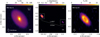 |
Fig. 1 Dust continuum emission imaged with observation LBl. Panels a and c show each disk individually in brightness temperature. The panel b shows both disks together in brightness per beam, and the projected distance at this epoch. The beam resolution is the same for all the panels, and its size is 18 × 30 mas, as shown in the lower left corner of panel a. The scale bar is 5 au at the distance of the source. |
3 Results
3.1 Dust continuum emission
The dust continuum observations are resolved into two independent disks (as it had been observed before in Cabrit et al. 2006; Rodriguez et al. 2018; Long et al. 2019; Manara et al. 2019), one disk around each source of the system, as shown in Fig. 1. When imaged at very high angular resolution, RW Aur A is resolved into a compact (R90% = 0.124″ or 19 au, with R90% the radius that encloses 90% of the dust continuum emission) centrally peaked disk, without evidence of an annular ring-like structure with the 3 × 5 au beam resolution. Located about 233 au in projected distance to the southwest is RW Aur B, which is also a compact disk (R90% = 0.093″ or 14 au) with evidence of a dust continuum ring. The sizes were constrained through visibility modeling of the dust continuum emission visibilities, as described in Sect. 3.2.
We constrained the flux of each source from the visibility modeling by integrating it from the model images. The dust continuum of RW Aur A is almost eight times brighter than that of its companion RWAurB, with 34.5 mJy and 4.4 mJy of integrated flux, respectively, as also shown in Table 2. RW Aur A is also considerably hotter in brightness temperature, with a peak Tb = 120 K in the disk center. The brightness temperature profile of RW Aur A decreases monotonically as a function of radii and remains higher than 20 K until a radius of 107 mas (or 17 au). In contrast, the maximum brightness temperature of RWAurB at any radii is 15 K. The azimuthally averaged brightness temperature profiles are shown in Fig. 2, and their amplitude difference is further discussed in Sect. 4.3.
For an estimate of the dust mass, we followed Hildebrand (1983):
 (1)
(1)
where d is the distance to the source, ν is the observed frequency, Bν is the Planck function at the frequency ν, and Kν = 2.3(ν/230 GHz)0.4 cm2g−1 is the frequency-dependent mass absorption coefficient (as in Andrews et al. 2013). The additional assumption for this calculation was that the dust emission at 1.3 mm is emitted by optically thin dust with a known temperature, that is commonly set to 20 K for standard reference (as in Ansdell et al. 2016; Cieza et al. 2019). As the brightness temperature is higher than 20 K for about 75% of the emitting area of RW Aur A, the assumption of optically thin emission fails, and we can therefore only provide a lower limit to its dust mass. When we assume a midplane temperature of 20 K (for comparison with other surveys and observations), we obtain a dust mass of 23.9 M⊕ and 3.1 M⊕ for A and B, respectively. Instead, with an average brightness temperature of RW Aur A within its R90% of 27 K, the dust mass becomes 16.4 M⊕.
Disks properties and relative astrometry from visibility modeling.
3.2 Continuum visibility modeling
To determine the dust continuum emission morphology and properties, we used the packages galario (Tazzari et al. 2017) and emcee (Foreman-Mackey et al. 2013) to fit a parametric visibility model to the data. We generated one independent image for each source and calculated the visibilities of each model separately. The additive properties of the Fourier transform allowed us to add the visibilities of each source and compare the combination to the observations.
We fit all the epochs at the same time with the same intensity models. However, we allowed the disk centers to be different in each observation, with the underlying assumption that each disk brightness distribution is constant during the 2 yr covered by our data, and the only possible difference between epochs are the relative disks positions.
Additionally, it is known that the ALMA flux calibration uncertainties can reach up to 10%, and even higher in particular cases (as in some of the DSHARP sources, Andrews et al. 2018). We therefore added a free parameter for each epoch, a scalar iobs ≈ 1, which multiplied the whole intensity model, and scaled the possible flux density difference. As a reference, we used observation SB4, which has a fixed iS B4 = 1, and thus, all the remaining iobs scaled the models to match the SB4 flux density. This epoch was chosen because it has the highest sensitivity in short baselines and is neither the brightest nor dimmest observation, as confirmed by the scaling factors iobs in Table A.1.
We fit azimuthally symmetric models to RW Aur A, and RW Aur B, taking the morphology of the CLEAN image and model as a guideline. For RW Aur A, the function used to describe its brightness profile is the following:
 (2)
(2)
where fA0 is the flux density of a point source at the disk center, G is a centrally peaked Gaussian with a peak flux of fA1 and a standard deviation of σA1, and TP is a power law tapered with an exponential decay, described in Appendix A. The point and Gaussian components are needed to describe the inner emission of the disk, and the tapered power law was used to describe the monotonically decreasing brightness decay with the possibility of a sharp outer edge, if needed.
For RW AurB, the disk is highly inclined and compact, and therefore, the information of its cavity is limited. A possible parameterization for the dust continuum ring could have been made with a broken Gaussian (i.e. a Gaussian ring with different widths for each side of its peak). However, this model returns a very steep inner edge to try to compensate for the slow decrease of its outer edge (similar to the inclined disk MHO 6 in Kurtovic et al. 2021). This problem with the broken Gaussian description can be overcome by slightly increasing the complexity of the model to two Gaussian rings. These Gaussians can become a centrally peaked emission while allowing the model to fit radially asymmetric rings. The equation that describes the model of RW Aur B as a function of radii is:
 (3)
(3)
where fB1 and fB2 are the peak intensity of each ring, centered at rB1 and rB2 with a Gaussian width of σB1 and σB2, respectively.
We ran a Markov Chain Monte Carlo (MCMC) fitting on all five epochs at the same time, to achieve complete visibility coverage starting from the 7m antennas of the ACA array from SB2, to the longest baselines from ALMA antenna configuration C-10 with LB1. We used a flat prior over the allowed parameter space, and the boundaries for each free parameter were wide enough such that walkers never interacted with them. The pixel size for the model images was initially 4 mas, and we also tested the stability of the fit by running the same models with a pixel size of 2 mas, from which we obtained consistent results. A summary of the main results is given in Table 2, and the remaining free parameters of the MCMC are shown in Table A.1.
By construction, the emission from RW Aur A is centrally peaked, and our model described the disk emission as a monotonically decreasing profile. When the residual visibilities were imaged (see Fig. 3), we found our flat-disk model described most of the structure detected in observation LB1, because the highest peak residual is only 6σ (compared to >300σ of the dust continuum image). Even though the residuals contrast are low, their structure suggests that our description of a Gaussian with a point source for the central emission is incomplete. A more detailed discussion of the residuals is given in Sect. 3.5.
Our model for RW AurB, on the other hand, completely describes the disk emission to the noise level, and no structured residual is detected at the position of the source (see Fig. 3). We find that the RWAurB ring peaks at about 42mas, which is 6.5 au from the disk center. Interestingly, both disks show a similar geometry in our line of sight, and their position angles are the same to the uncertainty level. RW Aur B is slightly more inclined than A, as was also estimated by Rodriguez et al. (2018) and Manara et al. (2019). Under the assumption that the angular momentum vector of both disks points to the same side of the sky plane, we find a misalignment of 9.15 deg, or 118.8 deg if they point in different directions.
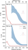 |
Fig. 2 Azimuthally averaged brightness temperature profile calculated from the CLEAN image of the dust continuum shown as dashed red lines. The brightness temperature profile for the 12CO is shown as a dotted blue line, as measured from the peak brightness LB image. The inner three beams have been excluded due to the brightness dilution in the channel maps. The colored regions show the 1σ dispersion at each location. The Gaussians in the right part of each panel represent the average radial resolution of the dust continuum image and LB 12CO. The beam sizes are shown in Fig. 1 and 7. |
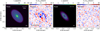 |
Fig. 3 Visibility modeling results. Panels (a) and (c) show the best parametric models for RW Aur A and B, respectively. Panels b and d show the image of the residual visibilities in units of the image sensitivity. The scale bar is 10 au at the distance of the source, and the beam size in the residual images is shown in the lower left corner. |
3.3 RW Aur B orbit: With ALMA astrometry
RW AurB shows a consistent trend of movement toward the southwest as a function of time. Assuming that the centers of the disks coincide with the location of the stars, we can use the visibility-modeled disk center as a precise astrometric measurement for each system. The uncertainty is considered to be the region including 68% of the MCMC solutions. This assumption implies that the disks are axisymmetric and have zero eccentricity, and we further discuss this in Sect. 4.6.
We combined our ALMA astrometry with the historical separation between RW Aur A and B as compiled by Csépány et al. (2017), covering epochs from 1944 to 2013. We excluded two outlier measurements from the historical astrometric positions: an observation from 1991 published in Leinert et al. (1993) that considerably deviates from the positional trend, and is inconsistent by about 0.1″ in separation and more than 2 deg in position angle with measurements from 1990 and 1994; and a measurement from 1944 by Joy & van Biesbroeck (1944) that does not provide uncertainties.
We included a single radial velocity (RV) measurement using the relative line-of-sight velocity obtained with ALMA, assigning an average epoch considering our four ALMA observations with equal weighting. This radial velocity was assigned to RWAurB with a value of −0.954 km s−1 (where negative means approaching us), relative to the reference rest frame of RW Aur A. Due to the high S/N of the emission of each disk in the 12CO channel maps, the integrated velocity images, such as moment 1 and velocity at peak brightness, show a “channelization problem”, where the low-frequency resolution produces a discrete velocity distribution instead of a continuous rotation map (the 12CO emission is further discussed in Sect. 3.6). This effect makes it challenging to obtain a meaningful uncertainty from the ALMA cube, and we therefore set a conservative 1σ dispersion to 100 ms−1 for the RV fitting.
To recover the orbit of RW Aur B around RW Aur A, we considered two different eccentricity regimes: elliptical orbits (ecc < 1), and hyperbolic orbits (ecc > 1). Both families of orbits were calculated using the Python package rebound (Rein & Liu 2012; Rein & Spiegel 2015). We created a simulation setup with a central mass at the origin of the coordinate system containing the cumulative mass of the binaries, and mass-less particles representing the position of RW Aur B. This is equivalent to a system in which each star has its own mass, and both move relative to an inertial coordinate system. The package rebound receives the true anomaly as input to set the position of a particle relative to the given orbital parameters, instead of physical time. Further details of the time-to-anomaly transformation for elliptical and hyperbolic scenarios are reported in Appendix B.
We sampled the probability density distribution of the orbital parameters using MCMC with emcee (Foreman-Mackey et al. 2013). The orbits were allowed to be either elliptical or hyperbolic with a uniform prior for any positive eccentricity, except for a small forbidden region around |1 − ecc| < 10−4 to avoid parabolic solutions. We fit the distance at periastron (dperi) instead of the semi-major (semi-transverse) axis “a” for elliptical (hyperbolic) orbits. By definition, a = dperi/(1 − ecc), which diverges for values of ecc ≈ 1 in either the elliptical or hyperbolic regime, introducing an undesired prior over the allowed eccentricity values. We used 24 times as many walkers as the number of free parameters, which were eight for a given orbit: the distance at periastron (dperi), the eccentricity (ecc), the inclination (inc), the longitude of the ascending node (Ω), the argument of periastron (ω), the time of the last periastron (tperi), the parallax (plx), and the total mass (mtot).
After running for over 107 steps per walker, we did not achieve convergence for each walker separately, in particular, in the low likelihood regime for Ω. The main reason for the delayed convergence is the highly correlated relations between the orbital parameters (as shown in Figs. A.2, A.3, and A.4). However, the probability density distribution derived from the walkers positions reached stable values after > 107 steps. After this stability was achieved, we ran an MCMC recording only one of every 80 steps to reduce data volume, and we derived the solutions from the last 105 recorded positions for every walker.
The orbital solutions are shown in Fig. 4, and their probability density distribution is presented in Fig. 5. In the appendix, we include the probability density distribution for each parameter after separating elliptical and hyperbolic solutions (see Fig. A.1). In Table 3, we detail the best values and their 1σ uncertainty. The orbital solutions with the highest likelihood are found in the eccentricity range between 0.5 and 0.95, but there is a tail of solutions with eccentricities >1 that are still allowed with the current astrometry, and thus, the hyperbolic solution is not ruled out.
Elliptical and hyperbolic solutions find different distributions for dperi and tperi, as shown separately in Fig. A.1. While elliptical solutions show closer dperi over a wider range of tperi, most hyperbolic solutions are only consistent with very recent tperi (some even in the near future) and large dperi, suggesting larger distances for the fly-by interaction. The values for dperi in the hyperbolic regime are considerably larger than three times the gas size of the disks (see also Fig. A.1), which makes these orbits less consistent with the truncation scenario, as we discuss further in Sect. 4.1. Additionally, hyperbolic orbits are only allowed for very narrow ranges for inc, Ω and ω.
The tperi located in the near future are not consistent with the brightest tidal arc in the 12CO emission, which must have resulted from close interaction (Dai et al. 2015). Thus, in Table 3, we also include the uncertainties after filtering the orbital solutions by tperi before the epoch of ALMA observations. The distributions after the filtering are also shown in Fig. A.1. For elliptical orbits, we estimate that the period is  yr, where the uncertainties represent the 1σ dispersion from the best solution. The large uncertainty for long-period orbits come from the orbits with ecc ≈ 1, as the semi-major axis of these orbits diverges.
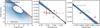 |
Fig. 4 1000 randomly sampled orbital solutions are shown from a larger field of view in the left panel, to a small zoomed region in the right panel. The solid dark line shows the solution with highest likelihood. The blue orbits are elliptical solutions, and the red orbits are hyperbolic solutions. The astrometry considered in this work is shown with red markers, and the position of RW Aur B with best model is shown as orange circles at the same epoch as the astrometric measurements. For reference, Gaia DR3 astrometry is shown with a gray square in the middle panel. The uncertainty from Gaia is smaller than the symbol size. |
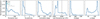 |
Fig. 5 Normalized probability density distribution for the fitted orbital parameters of RW Aur B around RW Aur A. For reference, the dashed lines in the left panel show the continuum, gas, and three times the gas size of RW Aur A, respectively. The last periastron year is shown in UTC, and the dashed line shows the time of the last observation. |
Orbital parameters of the RW Aur binary.
3.4 RW Aur B orbit: Excluding ALMA astrometry
Additional tests were run excluding the ALMA astrometry from the orbital fit. We fit the orbital parameters for three different scenarios: (i) Only with the historical astrometry from Csépány et al. (2017), (ii) with historical astrometry and the ALMA radial velocity, and (iii) with historical astrometry, the ALMA radial velocity, and the Gaia DR3 astrometry. We find that the historical astrometry by itself or the historical astrometry combined with the ALMA radial velocity are not able to constrain the eccentricity of the orbit. When combined with the astrometry from Gαiα DR3, the highest likelihood orbits are in the range ecc < 1, but the hyperbolic orbits are not excluded, similarly to the case of fitting the ALMA astrometry. The astrometry of both instruments was not combined in a single fit, because of a non-negligible difference in astrometry between ALMA and Gaia DR3 of about 6mas, which is shown in the middle panel of Fig. 4. This is further discussed in Sect. 4.
3.5 Inner disk geometry of RW Aur A
After we subtracted the best visibility model in Sect. 3.2, the residuals in the RW Aur A inner disk show a dipole-like structure (as shown in panel b) of Fig. 3), which could be due to a slightly different inclination for this region (see compilation of residuals in the Appendix of Andrews et al. 2021). On the other hand, the timescale for the latest binary interaction suggested by our orbital fitting was most likely few hundred years ago, which could have misaligned the geometry of the inner and outer disk. Motivated by these results, we ran an additional visibility model for the dust continuum emission in the same way as described in Sect. 3.2. We allowed the central Gaussian component describing the inner disk emission of RW Aur A to have a different inclination and position angle (incinn, PAinn) relative to the outer disk (incout, PAout). The results of the MCMC are shown in Table 4 and Fig. 6.
The central Gaussian finds a higher inclination than the outer disk, with a relative difference of 6.0 ± 0.4 deg between the inner and outer disk. The Gaussian width at half maximum is 3 au, indicating the extent of the tentative inner disk warp. When reconstructing an image with the residual visibilities between the observation and the best model, we find that the highest amplitude residual is 5σ, which is lower than for the non-warped disk model. Nonetheless, low-contrast residuals from non-axisymmetric structures are observed throughout the whole disk. The remaining parameters describing the outer disk of RW Aur A and RW Aur B remained consistent.
Geometry and inner disk properties of RW Aur A.
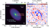 |
Fig. 6 As in Figure 3, but for the warped visibility model described in Sect. 3.5. The inner disk ellipse in panel a shows the full width at half maximum size of the central Gaussian, with the geometry from Table 4. |
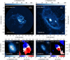 |
Fig. 7 12CO emission images at different spatial scales. Panel a shows the peak emission of each pixel, imaged by combining observations SB1, SB2, and SB4. Panel b shows the moment 0 image generated by combining all the existing datasets. Panels c to f were generated by clipping the emission at 1.3 mJy beam−1 m s−1, and panels c and d are a zoom into RWAur A, while panels e and f are a zoom into RW AurB. Panels d and f show the velocity of the peak brightness emission. The color bar of the velocity at peak has been chosen so that the central velocity matches the systemic velocity of each disk. The contour in panels c and e show the 5σ dust continuum contours. |
3.6 12CO J = 2−1 emission
Our12 CO observation redetects the main spiral arc reported in Cabrit et al. (2006). The increased sensitivity also allowed us to connect the clumps of emission detected in Rodriguez et al. (2018), previously called α, β, γ, and δ, into an intricate system of tidal arcs, filaments, and an extended diffuse background emission, which extends farther than 2000 au in projected distance from RWAur A, as shown in panel a in Fig. 7. This panel also shows the whole field of view of the SB 12CO image, which combines the observations with short baseline configurations (SB 1, SB2, and SB4), thus maximizing the sensitivity over extended spatial scales. The LB 12CO image is shown in panel b, and its increased angular resolution allowed us to resolve the disk emission and kinematics, shown in panels c to f. Component RW Aur C, proposed in Rodriguez et al. (2018), is not resolved into a disk-like emission or coherent rotating structure. As the LB 1 observation has a lower frequency resolution than the other observations, the LB 12CO image is limited to a velocity resolution of 1.3 km s−1, which hides kinematic structures with a smaller velocity amplitude.
We used the package eddy (Teague 2019a) to fit the Keplerian rotation of each disk and estimate the mass of the central object. We did not downsample the velocity image pixels, which have a size of 4 mas. The emission was masked using an elliptical mask with a size of 0.4″ and 0.28″ for A and B, respectively, to avoid including non-Keplerian emission that surrounds each object. As a result of the compact nature of the sources and the low-frequency resolution, our images cannot distinguish upper and lower emission surfaces. Therefore, we fit them with a flat Keplerian disk. The disk center, inclination, and position angle are fixed values from the dust continuum modeling, taking the values obtained for the outer disk. The only free parameters for each disk are the stellar mass and the central velocity in the line of sight. For RWAur A, we obtain MA = 1.238 M⊙ and VLSRA = 6172.44 m s−1, and for RWAurB we obtain MB = 0.995 M⊙ and VLSRA = 5218.24 m s−1. The two mass measurements are in agreement with spectroscopic estimates (Herczeg & Hillenbrand 2014; Long et al. 2019; Manara et al. 2019). The uncertainty estimate from eddy suggests that the standard deviations are a fraction of a percent for the masses and velocity in the local standard of rest. These small uncertainties come from the combination of the very high sensitivity per channel and the low-velocity resolution, which produces a “channelization” effect, as described in the second paragraph of Sect. 3.3, and shown in panels c to f from Fig. 7. A comparison of this masses with the position-velocity diagram of each binary is shown in Fig. 8. A possible solution of this problem is a forward-modeling of the image cube (e.g., Izquierdo et al. 2021), or of the visibilities (e.g., Long et al. 2021; Kurtovic & Pinilla 2024). For both approaches, a better understanding of the gas disk structure is needed. The possible misalignment of the inner disk was not considered in our fit, as the inner 3 au are completely contained within the first beam of the LB 12CO image, and it has therefore little influence on the mass estimate, which is mainly constrained by the outer disk.
The detected emission structures span thousands of astronomical units in spatial scales and about 40km s−1 in velocity. Over this extended range, many pixels in the image are part of different 12CO kinematic structures, such that a single velocity image at peak emission or moment 1 does not represent the kinematic richness of the gas. To alleviate this problem, we separated the channels into the blue- and redshifted emission relative to RW Aur A and calculated their peak brightness and velocities, as shown in Fig. E.1. Most of the redshifted emission is connected to the bright southern arc, while the blueshifted emission has a semi-circle shape, with most of the emission being northwest of RW Aur A. Under the assumption that these structures move farther away from the RW Aur disks, the northwestern emission would be closer toward us in the line-of-sight direction, and the redshifted southeastern emission would be farther away, as also proposed by Cabrit et al. (2006).
The high angular resolution 12CO moment 0 after continuum subtraction shows that neither of the disks is centrally peaked, as shown in Fig. 7. In RWAurB such morphology is expected, because there is a cavity in the dust continuum emission. However, it is unexpected in RW Aur A, where the dust continuum is centrally peaked. In this disk, the morphology of the 12CO moment 0 could be influenced by oversubtraction of an optically thick dust continuum emission and beam dilution in the central regions (e.g., Wölfer et al. 2021). When we measured the location of the peak emission in 12CO, we obtained a peak at 113 ± 4 mas (about 18 au) for RW Aur A and a peak at 93 ± 4 mas (about 15au) for RWAurB, roughly at the locations of their outer radii in the dust continuum emission. As the disks are surrounded by material from the interaction, the definition of the outer radii for the gas is not as simple as in isolated disks. To avoid including emission from the surrounding material, we integrated the flux over an elliptical aperture with a radius of 0.6″ and 0.45″ for RW Aur A and B, respectively. Farther than these distances, the flux contribution is dominated by the surrounding material, and not by the disks. The radii enclosing the 68% and 90% of the flux for RW Aur A are RA,CO,68% = 327 ± 25 mas and RA,CO,90% = 456 ± 64mas, and for RW AurB, we obtain RB,CO,68% = 238 ± 29 mas and RB,CO,90% = 343 ± 60 mas. These radii are smaller than those measured by Rota et al. (2022). The main difference is the cutoff radius for the integrated flux. When compared to the R90% of the continuum radius shown in Table 2), both disks have a gas-to-dust size ratio of 3.7, which is consistent with dust evolution by radial drift (Trapman et al. 2019; Zagaria et al. 2021). However, this value should be considered as an upper limit, because the gas radius was measured from a beam-convolved12 CO profile. It is relevant to note that the R90% could still be influenced by perturbed material at the outer edge of the disks, and the disk radii where the material follows Keplerian motion could be smaller.
We combined all the compact antenna observations (SB1, SB2, SB3, and SB4) to produce images for 13CO and C18O, using the same imaging parameters as the 12CO. We calculated their velocity-integrated maps after clipping by 3σ, and the results are shown in Fig. E.2. In the 13CO image, the sensitivity is high enough to detect emission from the southern arc, but in C18O, we only have a detection of the RW Aur A disk. The angular resolutions of these images are similar to that of the SB 12CO image, and therefore we cannot resolve the cavities or structures, if they exist.
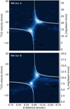 |
Fig. 8 Position velocity diagram calculated from the LB12 CO cube, using the inclination and position angle obtained with the dust continuum visibility modeling along the major axis. The dashed rotation curve shows the best solution obtained with eddy, while the shaded region shows the 3σ confidence region of the rotation curve by changing the stellar mass and disk systemic velocity, as discussed in 3.6. |
4 Discussion
4.1 Testing the bound/unbound nature of the RWAur system
The RW Aur binary system has two families of solutions that are consistent with the current astrometry: Bound orbit solutions, most of them in the eccentricity range between ecc ∈ [0.5 ~ 0.95], and unbound solutions with eccentricities extending up to ecc ≈ 3, as shown in Fig. 5, and Fig. A.1. There is a clear likelihood difference among the allowed orbits, with a group of elliptical orbits having a higher likelihood of describing the data than any of the hyperbolic orbits. We compare the solutions with the Akaike information criterion (AIC, Akaike 1974), which quantifies the loss of information for a given model. When comparing the best 99.85 percentile of elliptical and hyperbolic models, we find that the best hyperbolic models are 0.28 times as likely as the best elliptical models to be the solution that minimizes the information loss. Considering this probability in units of σ, there is a ~1.1σ of confidence that elliptical orbits are preferred over hyperbolic orbits. This comparison only takes into account the likelihood from the astrometric fit, and does not consider as a prior the morphology of the 12CO emission, which favors elliptical orbits to explain the extended emission.
When the elliptical and hyperbolic solutions are extended into the next decade, we predict that a single astrometric measurement is unlikely to distinguish between the bound or unbound solutions until after 2037 (see Fig. D.1), and thus, several measurements will be needed to continue to improve the orbit prediction. In radial velocity, both model families show a very small variation from the current measurement (< 0.1 km s−1) over the next two decades, which means that accurate astrometry will be the determining measurement to distinguish the nature of the RW Aur orbit. Because hyperbolic and elliptical orbits show distinct distributions of inc, Ω, and ω, a better constraint on any of these elements would also contribute to distinguishing the orbital eccentricity.
Future observations will improve our estimates for the distance at last periastron, which currently range between tens of au to about 600 au. When considering tperi to be older than the time of the ALMA observations, we find that tperi is most likely between 200 yr to 500 yr ago, although more recent periastrons are not been excluded with the current astrometry.
4.2 Evidence of interaction in the 12CO emission
Previous simulations of a close encounter in RWAur have shown that an interaction could excite tidally stripped arcs of material, such as the one observed in the 12CO emission (Dai et al. 2015). The additional clumps of 12CO detected by Rodriguez et al. (2018) that we redetected at higher sensitivity (see panel a in Fig. 7) could have been produced as tidal arcs in previous interactions of this bound system, which would be consistent with the elliptical orbit solutions.
Tidal interactions are expected to truncate the disks sizes, and simulations and analytical studies both found that disks in multiple stellar systems are truncated to a fraction of the binary separation (typically 0.3–0.5, e.g., Clarke & Pringle 1993; Pichardo et al. 2005; Harris et al. 2012; Rosotti et al. 2014; Manara et al. 2019; Zurlo et al. 2020; Zagaria et al. 2023). In RWAur, about 18% of the elliptical orbit solutions suggests that the distance at the closest interaction could be smaller than the measured gas extent (see Fig. 5), which contradicts the truncation scenario. Additional observations are needed for a more robust constraint on the size of the Keplerian disk around each star, and thus, to properly test their dynamical truncation.
When the orbital plane of the binary stars is not aligned with the plane of their disks, a warp can be excited during a close interaction (e.g., Papaloizou & Terquem 1995; Cuello et al. 2019; Nealon et al. 2020; Gonzalez et al. 2020). As the gravitational influence of the perturber decreases over time after periastron, the warp can smooth out toward coplanarity (e.g., Picogna & Marzari 2014; Martin et al. 2019; Rowther et al. 2022), and change the disk plane during this process. When we assume that the binary orbit is elliptical, then the circumstellar material will change their relative disk-binary inclination with every interaction, and thus, the next tidally stripped arc of material could be ejected in a different direction. This effect, added to possible temperature differences due to stellar illumination (e.g., Weber et al. 2023), are tentative explanations for the 12CO emission structure.
When the LB1 observation is included, both disks are spatially resolved in 12CO, allowing us to analyze their Keplerian rotation. Due to the low-frequency resolution, we are unable to confirm or exclude warped or tidally induced velocity structures, as has been observed in other systems (e.g., Kurtovic et al. 2018; Mayama et al. 2018). Additional high angular resolution observations toward RW Aur at a higher frequency resolution could explore this kinematic aspect of the interaction, and also allow us to estimate each stellar mass more robustly.
Neither disk is centrally peaked in the12 CO integrated intensity map, as shown in panels c and e in Fig. 7. In RWAurB, a cavity is also observed in the dust continuum emission. In RW Aur A, however, the dust continuum emission is centrally peaked, and a cavity in the gas emission is accordingly puzzling. As the peak emission of 12CO in RW Aur A is detected at a similar distance as the outer disk continuum radius, an optically thick dust continuum emission could result in a continuum oversubtraction, thus contributing to the observed cavity. However, the role of the accretion events, inner disk misalignment, and the possible asymmetry in the morphology of 12CO remains an open question. Observations at similar angular resolution to LB1 but at higher frequency resolution should be able to characterize the disk gas morphology, which would also allow us to determine the orientation of the inner disk from kinematics.
4.3 Disks structure in dust continuum emission
We confirm the compact nature of the dust continuum disk sizes, as was also observed by Rodriguez et al. (2018) and Manara et al. (2019). Although the RW Aur A dust continuum image (as reconstructed by CLEAN) seems to be a featureless disk, the residuals from our visibility modeling show that it is rich in low-contrast small-scale structure. A geometrically flat disk model describes most of the emission of the disk, and it only leaves a strong structured residual in the inner disk region, suggesting a different inclination for inner and outer disk. From an additional visibility modeling, in which we allowed the inner disk region emission to have a different inclination, we find a difference of 6.0 ± 0.4 deg between the inner (<3 au) and outer disk (>3 au) and a difference in PA of 4.0 ± 0.6 deg. This tilt could have originated in the last close encounter between the two stars. Additional structure is observed in the residual map after subtracting the model with a misaligned inner disk (see Fig. 6), suggesting that the inner disk of RW Aur A could have an azimuthally asymmetric structure, as was observed in the inner disk of other systems (e.g., GRAVITY Collaboration 2024). Higher angular resolution observations are needed to confirm this geometry and morphology, and this makes RWAur A an ideal candidate for observations with the near-infrared interferometric capabilities of the Very Large Telescope.
The misalignment we observe in RW Aur A is likely to be smaller than the initial tilt induced by RWAurB during the last periastron. With SPH simulations, Rowther et al. (2022) showed that the timescale for smoothing out a misalignment can be as short as a few orbits of the outer disk edge, which is consistent with the time since last periastron recovered with our orbital fittings. Rowther et al. (2022) also showed that the difference in the velocity field between the inner and outer warped disk can produce work and dissipate energy as heat. Under the assumption of optically thick dust continuum emission, the misalignment might contribute to the high brightness temperature observed in the midplane of RW Aur A.
More generally, the evolution of a warped structure over time depends on the viscosity of a disk, and in the low-viscosity regime, a warp can have a wave-like behavior (Lubow & Ogilvie 2000; Martin et al. 2019; Dullemond et al. 2022; Kimmig & Dullemond 2024). Koutoulaki et al. (2019) explored the role of a misalignment between inner and outer disk in the dimming events that have been observed since 2010, showing that for a disk with T = 30 K at 10 au and a bending-wave starting at 58 au, the warp would take about 520 yr to reach the inner disk. The last periastron passage derived from the elliptical orbits with the ALMA astrometry is consistent in order of magnitude with this estimate ( yr from the beginning of 2024), and is also consistent with the last periastron of the hyperbolic orbits. Additionally, our findings indicate that the inner 3 au show a higher inclination than the outer 3 au disk, which supports the hypothesis that material in a misaligned inner disk contributes to the dimming events (Facchini et al. 2016).
Considering the results of our elliptical and hyperbolic orbital fitting, we can speculate about the origin of the dust structures in the disk of RW Aur B. The distribution of elliptical solutions for the binary periastron distance accumulates at small radii, with a peak likelihood comparable to the gas radii of RW Aur A, with orbital solutions as small as their dust size. These orbits are not consistent with expected disk truncation from close interactions, and no strong constraints over the minimum interaction distance can be set with the current astrometric data. These small dperi do not exclude the possibility of a disk collision, although it should be noted that we cannot infer the disk size before the periastron, and similarly, we also find solutions for the periastron that are larger than the emission radii and are more consistent with dynamical truncation.
The close encounter, elliptical or hyperbolic, would have induced a warp in RW Aur A, while RW Aur B could have captured some material into its own disk (even if the perias-tron is larger than the disk size, Clarke & Pringle 1993), as was observed in SPH simulations of fly-by encounters (e.g., Dai et al. 2015; Cuello et al. 2019; Gonzalez et al. 2020). The lower surface density of captured grains could translate into a lower optical depth, which is consistent with the low brightness temperature of RW Aur B. The captured material scenario could be tested with dedicated simulations using the recovered orbital parameters and the observed geometry of the two disks.
Our speculative interpretation of the disk structures would benefit from additional observations at high angular resolution. A follow-up with ALMA starting from cycle 11 would increase the time baseline of the ALMA astrometry by a factor of four compared to this work, and it would allow a more robust determination of the time and distance at periastron, for either the bound or unbound solutions. Similarly, a follow-up in longer millimeter wavelengths will enable accurate measurements of the spectral index and optical depth, which could provide an additional test of our explanations for the origin of the substructures by better constraining the dust density and temperature distribution of each disk.
4.4 Orientation of the orbit, disks, and jet emission
The geometry of each disk is constrained based on our dust continuum observations. Additionally, we spatially resolve the blueand redshifted sides in the 12CO kinematics (see Fig. 7). Our angular and frequency resolution are not high enough to differentiate between the upper and lower emission layers of the disk, and consequently, we are unable to determine the orientation of the angular momentum vector for each of them using only the CO emission. However, RW Aur A has a well-studied jet with a redshifted component oriented in the northwest direction (Dougados et al. 2000). Assuming that the disk is close to perpendicular to the jet (as it has been observed in other young sources, e.g., Burrows et al. 1996; Flores-Rivera et al. 2023), we can infer from the rotation map shown in Fig. 7 that the angular momentum vector of RW Aur A points in the northwest direction as well, which results in a clockwise rotation of the disk in the sky plane.
In a coordinate system centered on RW Aur A, RW Aur B also orbits in clockwise orientation. When we compare the inclination and position angle of RW Aur A disk, using the orientation implied by the jet emission, with the inclination and longitude of the ascending node of the orbital solutions from the MCMC, we obtain a disk-binary misalignment of 27.1 ± 26.7 deg, where the errors represent the 1σ dispersion around the best value. The last interaction was most likely at a prograde orientation relative to RW Aur A, although more polar interactions up to a misalignment of ≈70 deg are not ruled out. We exclude the scenario of a strong retrograde interaction.
4.5 Origin of the close interactions
There are a few speculative scenarios for the origin of the close interactions. For example, if the last interaction was hyperbolic in nature, then the stars would be gravitationally unbound before and after the interaction, also known as a fly-by. Even though this scenario is not excluded with the current astrometric measurements, it is more challenging to reconcile with the multiple filaments and features observed in the 12CO emission.
We can also consider the hypothesis that the RW Aur binary has only recently been induced into a highly eccentric elliptical orbit. This could have occurred through stellar capture from an initially unbound interaction, as proposed by Rodriguez et al. (2018), or alternatively, RW Aur A and B could have been induced into a highly eccentric elliptical orbit through an interaction with a third body. The dissolution of triple stellar systems commonly results in the formation of a single and a binary stellar system (e.g., Toonen et al. 2022), and interactions with external gravitational potentials (e.g., a third companion) can change the eccentricity of the bound binary (e.g., Monaghan 1976; Stone & Leigh 2019; Ginat & Perets 2021).
By analyzing Gaia DR3 proper motion and parallax, Shuai et al. (2022) found that Gaia DR3 156431440590447744 could have had a closest approach at a distance of 13.2 ± 2.5 kau with RW Aur about 6 ⋅ 103 yr ago. Although this large distance makes an interaction unlikely, both RW Aur A and RW Aur B have Gaia RUWE values over 1.4 (16 and 1.5 respectively), and thus their parallax and proper motion should be reanalyzed in future works considering their binarity and variability. Observations over a longer time baseline with high-precision parallax measurements could test this third-companion hypothesis and potentially improve our constraints on the dynamical history of the RW Aur binary.
4.6 Astrometry with ALMA
Due to their compact emitting surface, stars are usually undetected in millimeter-wavelength observations. As stars cannot be directly observed with instruments such as ALMA, it is challenging to find a reference for high-precision astrometry. When binary disks are detected, as in RW Aur, high-precision astrometry can be performed in a relative coordinate system by fixing the origin on the center of one of the disks and calculating their relative separation.
The center of each disk can be recovered with MCMC approaches such as parametric visibility modeling. To translate disk astrometry into stellar astrometry, we need the additional assumption that the stars are in the center of the disks. Even though this is a safe assumption for most of the study cases, ALMA is sensitive to very low contrast asymmetries and eccentricity structures (e.g., Andrews et al. 2021; Kurtovic et al. 2022), which could shift a disk center by a few milliarcseconds. Thus, any attempt to recover stellar astrometry from modeling the disk’s position must use a model that describes the emission morphology as well as possible.
In RW Aur A, our parametric model for the dust continuum did not consider azimuthal asymmetries at any radius, which left low-contrast structure in the residual image (see Fig. 6). These residuals are problematic, because an asymmetry in the inner disk region could slightly shift the recovered center of the disk. We considered an azimuthally symmetric disk brightness distribution with a flux of Ls, with a compact asymmetry in the inner disk region of brightness La and a distance from the geometric center ra. The shift of the disk light center rlc from the geometric center will be rlc = raLa/(Ls + La). For an asymmetry at ra ≈ 1 au, the shift of RW Aur A would be rlc ≈ 0.19La with La in mJy and rlc in milliarcseconds. Thus, over the span of a single orbit, an asymmetry of La ≈ 2.5 mJy could shift the light-center as much as 1 mas, which would modify the recovered disk center compared to an axisymmetric model. This effect is a possible explanation for the difference in relative astrometry between the observations SB1-LB1 and LB1-SB4, which do not show the same relative movement between the fitted disk centers even though they have a similar time baseline. Longer time baselines for astrometry should be less sensitive to asymmetries rotation.
In addition to carefully describing the disk morphology, additional considerations should be taken when recovering the relative disk astrometry from ALMA data. For example, the visibility weights of observations from different ALMA cycles should be standardized with tools such as statwt from CASA before they are compared with an MCMC-based approach. As the flux calibration of ALMA can vary by up to 10%, a flux-scaling factor should always be fit as part of the analysis process. Finally, if astrometry is the goal of an observation, the S/N should be high enough to be self-calibrated by itself, without the need of combining it with another observation that was taken at a different epoch.
For RW Aur, all of our observations were taken at almost the same frequency range (see Table 1), and we therefore assumed that the emission morphology was the same for every observation (neglecting the possible changes due to inner disk rotation discussed in the previous paragraphs). Attempts to obtain relative astrometry with parametric models from observations taken at different wavelengths should consider the wavelength dependence of the emission morphology, as structures can change in optical depth, and thus different regions of the disks do not necessarily have the same spectral index. In this scenario, a single flux-scaling factor will not work properly.
The relative binary motion from ALMA has conflicting values when compared to that from Gaia DR3, which prevents a simultaneous fit. A likely explanation for their difference are the systematics from Gaia when analyzing stars with circum-stellar material and variable brightness, quantified by the high RUWE values (Fitton et al. 2022), and the possible shifts due to asymmetries in the inner disk region. The RUWEs of RW Aur A and B are respectively 16 and 1.5, respectively, which is above the robustness threshold considered by Fabricius et al. (2021). The stellar occultation events in RW Aur A during the observing period of Gaia DR3 might also have introduced systematic errors in the AB relative positions, as well as the ejection of jet knots every 2–6 yr (Takami et al. 2020). Additional observations with ALMA and a reanalysis of the Gaia data should alleviate this issue.
When a high S/N observation with ALMA antenna configuration C-10 is analyzed, we obtain binary relative distances with an accuracy comparable to that of Gaia DR3. Thus, ALMA observations arise as an alternative for studying binary motion in young star-forming regions in which optical wavelengths are completely extincted by cloud contamination. Dedicated continuum observations at high angular resolution of regions such as Ophiuchus would allow us to study the impact of binarity and interaction in the very early stages of planet and star formation.
Another relevant approximation taken in this work was to consider the stars as point sources that contained all of the mass of the system, thus neglecting the mass distribution and contribution of their disks and surroundings. Considering the compact nature of the disks, and that the disk mass fraction is typically considered to be <0.05 M⋆, we find that a possible contribution from the disk masses would be within the uncertainty of the total system mass. However, the validity of this approximation should be considered separately for each case-study.
5 Conclusions
We analyzed the 1.3 mm emission of the RW Aur system, as observed by ALMA over a span of 2 yr, with angular scales ranging from the ACA-7m array to the ALMA C-10 antenna configuration. We resolved the disks in continuum and in 12CO emission, and confirmed their compact nature. When analyzed in the visibility plane, RW Aur A shows evidence of low-contrast non-axisymmetric structures, and the inner 3 au of the disk are tentatively misaligned by 6 deg relative to the outer disk. RW Aur B is well described by a single ring that peaks at 6 au in the dust continuum emission and shows a very low brightness temperature compared to RW Aur A.
Our 12CO observations at high angular resolution allowed us to constrain the binary mass under the assumption of Keplerian rotation for their disks. By analyzing the relative separation of the disks as a function of time and combining ALMA with historical astrometry and stellar mass, we constrained the allowed orbital parameter space for the RW Aur binary. We find that the most likely solutions are in the elliptical regime (gravitation-ally bound), indicating to a periastron epoch about 295 yr ago, but hyperbolic solutions (gravitationally unbound) are not yet excluded.
When fitting elliptical orbits, both models with the ALMA astrometry or Gaia DR3 astrometry find consistent results, with highly eccentric gravitationally bound orbits. The hyperbolic models become more likely when approaching ecc = 1 from above. Overall, elliptical and hyperbolic solutions agree that the last periastron did not occur more than ≈ 500 yr ago, which is very recent in astronomical times. The tentative warp of RW Aur A and the brightness temperature structure of both disks are consistent with this very close interaction, whether bound or unbound. Additional observations are needed to confirm or reject this hypothesis, and should mainly be focused on obtaining a better constraint of the distance at last periastron and the physical properties of each disk.
The gas emission of RW Aur is resolved into an intricate system of extended low surface brightness emission and filamentary structures, which could be evidence of several close interactions, as previously proposed by Rodriguez et al. (2018), thus supporting the elliptical solutions over the hyperbolic case. Due to the limited frequency resolution of our observations, we are unable to confirm warped structures in the gas emission.
Multiple-epoch observations of binary systems with ALMA are a viable alternative to recover the stellar orbital parameters, which are crucial for understanding the impact of multiplicity on the planet formation potential of each disk. Even though careful visibility modeling is needed to recover robust disk astrometry, ALMA observations can be used as an alternative to Gaia in systems in which optical emission is entirely extinct, thus positioning ALMA as an ideal tool to follow young binary disks over the long term.
Acknowledgments
N.K. and P.P. acknowledges support provided by the Alexander von Humboldt Foundation in the framework of the Sofja Kovalevskaja Award endowed by the Federal Ministry of Education and Research. S.F. is funded by the European Union under the European Union’s Horizon Europe Research & Innovation Programme 101076613 (UNVEIL). CFM is funded by the European Union (ERC, WANDA, 101039452). Views and opinions expressed are however those of the author(s) only and do not necessarily reflect those of the European Union or the European Research Council Executive Agency. Neither the European Union nor the granting authority can be held responsible for them. This project has received funding from the European Research Council (ERC) under the European Union’s Horizon 2020 research and innovation programme (PROTOPLANETS, grant agreement No. 101002188). R.B. is acknowledges support from the Royal Society in the form of a University Research Fellowship. C.N.K. acknowledges funding from the DFG research group FOR 2634 “Planet Formation Witnesses and Probes: Transition Disks” under grant DU 414/23-2 and KL 650/29-1, 650/29-2, 650/30-1. This paper makes use of the following ALMA data: ADS/JAO.ALMA#2015.1.01506.S, ADS/JAO.ALMA#2016.1.00877.S, ADS/JAO.ALMA#2016.1.01164.S, ADS/JAO.ALMA#2017.1.01631.S, ADS/JAO.ALMA#2018.1.00973.S. ALMA is a partnership of ESO (representing its member states), NSF (USA) and NINS (Japan), together with NRC (Canada), MOST and ASIAA (Taiwan), and KASI (Republic of Korea), in cooperation with the Republic of Chile. The Joint ALMA Observatory is operated by ESO, AUI/NRAO and NAOJ.
Appendix A Dust continuum parametric models
The dust continuum emission of RW Aur A is described with a point source, a centrally peaked Gaussian and a tapered power law function. The tapered power law is shown in Eq. A.1, where the free parameters are the flux amplitude fA2, a critical radius RA2, and two exponents (α,β). The best values and 1σ uncertainty obtained from the visibility model are shown in Table A.1
![Mathematical equation: $TP\left( {r,{f_{A2}},{R_{A2}},\alpha ,\beta } \right) = {f_{A2}}{\left( {{r \over {{R_{A2}}}}} \right)^\alpha }\left( {1 - \exp \left[ {{{\left( {{r \over {{R_{A2}}}}} \right)}^\beta }} \right]} \right)$](/articles/aa/full_html/2024/12/aa47583-23/aa47583-23-eq21.png) (A.1)
(A.1)
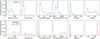 |
Fig. A.1 Same as Fig. 5, but showing the solutions with elliptical orbits in the upper panels, and with hyperbolic orbits in the lower panels. Hyperbolic solutions where the periastron epoch was before the first ALMA observation are shown with orange dashed line. Vertical lines in the left panel are as in Fig. 5. |
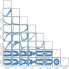 |
Fig. A.2 Corner plot of all orbital solutions. |
Visibility modeling results for the dust continuum emission.
Appendix B Orbital solutions
The package rebound (Rein & Liu 2012; Rein & Spiegel 2015) was used to calculate the coordinates of RW Aur B given a set of orbital parameters. This was done by including a point mass at the origin of the coordinate system, containing the combined mass of the binaries and massless particles representing the position of RW Aur B at the time of each observation. We did not utilize the simulation capabilities of rebound, which can evolve the positions running a numerical simulation. These massless particles shared the same orbital parameters and would only differ in their true anomaly, which we will refer to in this Section as “ν”. The value of ν represents the angular distance between the current particle position and the vector pointing from the origin to the periastron of the orbit.
For a given set of orbital parameters, the value of ν can be measured for each astrometric measurement. However, describing it as a function of physical time ν := ν(t) is relevant to compare the astrometry of each observed epoch. Even though there are Python packages to calculate orbital positions as a function of time for elliptical orbits (e.g., orbitize !, Blunt et al. 2020), most of the currently available tools to calculate hyperbolic orbits are made to calculate orbits with ν as input. In the following, we summarize the steps we took to go from time to ν.
First, we calculate the mean angular motion “n” as a function of the total mass of the system “mtot” and the hyperbolic semi-transverse axis “a”:
 (B.1)
(B.1)
where G is the gravitational constant, and a < 0 by definition. In our MCMC, the value of a is calculated from dperi and ecc as a = dperi/(1 − ecc). From n, we can calculate the mean anomaly “M“, as:
 (B.2)
(B.2)
where tper is the physical time of periastron, and t is the time of the measurement. The units of time of t must be the same as those of G. Next, the hyperbolic anomaly “F“ of a measurement is related to M by following:
 (B.3)
(B.3)
which has no analytical solution when solving F from M. Instead, we solve this equation numerically by using the Newton’s method, where:
 (B.4)
(B.4)
which we iterate in k until the difference |Fk+1 − Fk| is below 10−8 deg. We use as initial guess F0 = M. From the hyperbolic anomaly F, we finally derive the true anomaly ν as:
 (B.5)
(B.5)
thus completing the transformation of time at observation of each astrometric measurement to true anomaly ν, which is used as input to recover the coordinates and velocity at each point of the hyperbolic orbit.
For consistency, we also used rebound to calculate the elliptical orbits. Thus, we follow a similar procedure to go from ν to time. The mean angular motion is now calculated as:
 (B.6)
(B.6)
which is used to obtain the mean anomaly M. The relation between the elliptical anomaly E and M is:
 (B.7)
(B.7)
which we also solve with the Newton’s method. This E is used to obtain the true anomaly ν.
It is relevant to note that the semi-major axis for elliptical orbits, and semi-transverse axis for hyperbolic orbits, is a quantity that diverges for ecc = 1. Thus, we chose to run the MCMC with the distance at periastron instead of the semi-major (semi-transverse) axis, which are related through the eccentricity by:
 (B.8)
(B.8)
Appendix C Comparison of elliptical and hyperbolic orbits
In Fig. C.1, the histograms of the AIC (Akaike Information Criterion) is shown for the walkers with ecc < 1 (elliptical) and ecc > 1 (hyperbolic).
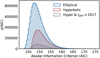 |
Fig. C.1 Histogram of the AIC value for all walkers, separated by elliptical, hyperbolic, and hyperbolic orbits where the periastron time is before the first ALMA observation. |
Appendix D Predicted astrometry
The orbital solutions derived in Sect. 3.3 allow us to predict the future position of RW Aur B, which we show in Fig. D.1. Given the current astrometric measurements, a single astrometric measurement will most likely not be enough to distinguish between elliptical and hyperbolic solutions. Several measurements over the years will be needed to constrain the nature of the RW Aur orbit.
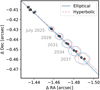 |
Fig. D.1 Predicted location of RW Aur B based on the elliptical (solid blue) and hyperbolic (dashed red) models, starting from July 2025, and then the July every three years until 2037. The position from the best elliptical and hyperbolic model are shown with a circles, while the contours show the 3σ scatter for each family or orbits. |
Appendix E RW Aur CO isotopologues emission
The velocity map of RWAur CO isotopologues are shown in Fig. E.1 and Fig. E.2. The 13CO J=2-l emission is detected in both disks, and the bright tidal arm to the south of RW Aur A is detected too. In C180 J=2-l emission, only RW Aur A is detected. Due to the moderate angular resolution of these detections, it is not possible to explore the radial morphology of the emission with the same detail as the dust continuum or 12CO J=2-l emission.
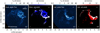 |
Fig. E.1 The 12CO blueshifted emission with respect to RW Aur A is shown in panels (a) and (b), while the redshifted component is shown in (c) and (d). The beam size in the lower left corner and the scale bar in the upper right are the same for all the panels. The centers of the 2 disks are shown with black + symbols. |
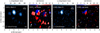 |
Fig. E.2 13CO Moment 0 and velocity at peak flux are shown in panels (a) and (b), while the same images for C18O are shown in panels (c) and (d). Beam sizes are shown in lower left corner, and a scale bar of 20 au is shown in the upper right corner. |
References
- Akaike, H. 1974, IEEE Trans. Automatic Control, 19, 716 [CrossRef] [Google Scholar]
- Alves, F. O., Caselli, P., Girart, J. M., et al. 2019, Science, 366, 90 [NASA ADS] [CrossRef] [Google Scholar]
- Andrews, S. M., Rosenfeld, K. A., Kraus, A. L., & Wilner, D. J. 2013, ApJ, 771, 129 [Google Scholar]
- Andrews, S. M., Huang, J., Pérez, L. M., et al. 2018, ApJ, 869, L41 [NASA ADS] [CrossRef] [Google Scholar]
- Andrews, S. M., Elder, W., Zhang, S., et al. 2021, ApJ, 916, 51 [NASA ADS] [CrossRef] [Google Scholar]
- Ansdell, M., Williams, J. P., van der Marel, N., et al. 2016, ApJ, 828, 46 [Google Scholar]
- Artymowicz, P., & Lubow, S. H. 1994, ApJ, 421, 651 [Google Scholar]
- Bate, M. R. 2018, MNRAS, 475, 5618 [Google Scholar]
- Blunt, S., Wang, J. J., Angelo, I., et al. 2020, AJ, 159, 89 [NASA ADS] [CrossRef] [Google Scholar]
- Bozhinova, I., Scholz, A., Costigan, G., et al. 2016, MNRAS, 463, 4459 [NASA ADS] [CrossRef] [Google Scholar]
- Burrows, C. J., Stapelfeldt, K. R., Watson, A. M., et al. 1996, ApJ, 473, 437 [Google Scholar]
- Cabrit, S., Pety, J., Pesenti, N., & Dougados, C. 2006, A&A, 452, 897 [CrossRef] [EDP Sciences] [Google Scholar]
- Chou, M.-Y., Takami, M., Manset, N., et al. 2013, AJ, 145, 108 [Google Scholar]
- Cieza, L. A., Ruíz-Rodríguez, D., Hales, A., et al. 2019, MNRAS, 482, 698 [Google Scholar]
- Clarke, C. J., & Pringle, J. E. 1993, MNRAS, 261, 190 [Google Scholar]
- Csépány, G., van den Ancker, M., Ábrahám, P., et al. 2017, A&A, 603, A74 [EDP Sciences] [Google Scholar]
- Cuello, N., Dipierro, G., Mentiplay, D., et al. 2019, MNRAS, 483, 4114 [Google Scholar]
- Cuello, N., Ménard, F., & Price, D. J. 2023, Eur. Phys. J. Plus, 138, 11 [NASA ADS] [CrossRef] [Google Scholar]
- Czekala, I., Loomis, R. A., Teague, R., et al. 2021, ApJS, 257, 2 [NASA ADS] [CrossRef] [Google Scholar]
- Dai, F., Facchini, S., Clarke, C. J., & Haworth, T. J. 2015, MNRAS, 449, 1996 [Google Scholar]
- Dodin, A., Grankin, K., Lamzin, S., et al. 2019, MNRAS, 482, 5524 [NASA ADS] [CrossRef] [Google Scholar]
- Dong, R., Liu, H. B., Cuello, N., et al. 2022, Nat. Astron., 6, 331 [NASA ADS] [CrossRef] [Google Scholar]
- Dougados, C., Cabrit, S., Lavalley, C., & Ménard, F. 2000, A&A, 357, A61 [NASA ADS] [Google Scholar]
- Dullemond, C. P., Kimmig, C. N., & Zanazzi, J. J. 2022, MNRAS, 511, 2925 [NASA ADS] [CrossRef] [Google Scholar]
- Fabricius, C., Luri, X., Arenou, F., et al. 2021, A&A, 649, A5 [NASA ADS] [CrossRef] [EDP Sciences] [Google Scholar]
- Facchini, S., Manara, C. F., Schneider, P. C., et al. 2016, A&A, 596, A38 [NASA ADS] [CrossRef] [EDP Sciences] [Google Scholar]
- Fernández-López, M., Zapata, L. A., & Gabbasov, R. 2017, ApJ, 845, 10 [CrossRef] [Google Scholar]
- Fitton, S., Tofflemire, B. M., & Kraus, A. L. 2022, RNAAS, 6, 18 [NASA ADS] [Google Scholar]
- Flores-Rivera, L., Flock, M., Kurtovic, N. T., et al. 2023, A&A, 670, A126 [NASA ADS] [CrossRef] [EDP Sciences] [Google Scholar]
- Foreman-Mackey, D., Hogg, D. W., Lang, D., & Goodman, J. 2013, PASP, 125, 306 [Google Scholar]
- Gahm, G. F., Petrov, P. P., Duemmler, R., Gameiro, J. F., & Lago, M. T. V. T. 1999, A&A, 352, L95 [NASA ADS] [Google Scholar]
- Gaia Collaboration (Prusti, T., et al.) 2016, A&A, 595, A1 [NASA ADS] [CrossRef] [EDP Sciences] [Google Scholar]
- Gaia Collaboration (Brown, A. G. A., et al.) 2021, A&A, 649, A1 [NASA ADS] [CrossRef] [EDP Sciences] [Google Scholar]
- Ginat, Y. B., & Perets, H. B. 2021, MNRAS, 508, 190 [NASA ADS] [CrossRef] [Google Scholar]
- Gonzalez, J.-F., van der Plas, G., Pinte, C., et al. 2020, MNRAS, 499, 3837 [Google Scholar]
- GRAVITY Collaboration (Ganci, V., et al.) 2024, A&A, 684, A200 [NASA ADS] [CrossRef] [EDP Sciences] [Google Scholar]
- Harris, R. J., Andrews, S. M., Wilner, D. J., & Kraus, A. L. 2012, ApJ, 751, 115 [Google Scholar]
- Herczeg, G. J., & Hillenbrand, L. A. 2014, ApJ, 786, 97 [Google Scholar]
- Hildebrand, R. H. 1983, QJRAS, 24, 267 [NASA ADS] [Google Scholar]
- Izquierdo, A. F., Testi, L., Facchini, S., Rosotti, G. P., & van Dishoeck, E. F. 2021, A&A, 650, A179 [NASA ADS] [CrossRef] [EDP Sciences] [Google Scholar]
- Jorsater, S., & van Moorsel, G. A. 1995, AJ, 110, 2037 [Google Scholar]
- Joy, A. H., & van Biesbroeck, G. 1944, PASP, 56, 123 [NASA ADS] [CrossRef] [Google Scholar]
- Kimmig, C. N., & Dullemond, C. P. 2024, A&A, 689, A45 [NASA ADS] [CrossRef] [EDP Sciences] [Google Scholar]
- Koutoulaki, M., Facchini, S., Manara, C. F., et al. 2019, A&A, 625, A49 [NASA ADS] [CrossRef] [EDP Sciences] [Google Scholar]
- Kurtovic, N. T., & Pinilla, P. 2024, A&A, 687, A188 [NASA ADS] [CrossRef] [EDP Sciences] [Google Scholar]
- Kurtovic, N. T., Pérez, L. M., Benisty, M., et al. 2018, ApJ, 869, L44 [Google Scholar]
- Kurtovic, N. T., Pinilla, P., Long, F., et al. 2021, A&A, 645, A139 [EDP Sciences] [Google Scholar]
- Kurtovic, N. T., Pinilla, P., Penzlin, A. B. T., et al. 2022, A&A, 664, A151 [NASA ADS] [CrossRef] [EDP Sciences] [Google Scholar]
- Leinert, C., Zinnecker, H., Weitzel, N., et al. 1993, A&A, 278, 129 [NASA ADS] [Google Scholar]
- Long, F., Herczeg, G. J., Harsono, D., et al. 2019, ApJ, 882, 49 [Google Scholar]
- Long, F., Andrews, S. M., Vega, J., et al. 2021, ApJ, 915, 131 [NASA ADS] [CrossRef] [Google Scholar]
- Lubow, S. H., & Ogilvie, G. I. 2000, ApJ, 538, 326 [CrossRef] [Google Scholar]
- Manara, C. F., Tazzari, M., Long, F., et al. 2019, A&A, 628, A95 [NASA ADS] [CrossRef] [EDP Sciences] [Google Scholar]
- Martin, R. G., Lubow, S. H., Pringle, J. E., et al. 2019, ApJ, 875, 5 [NASA ADS] [CrossRef] [Google Scholar]
- Mayama, S., Tamura, M., Hanawa, T., et al. 2010, Science, 327, 306 [NASA ADS] [CrossRef] [Google Scholar]
- Mayama, S., Akiyama, E., Panic, O., et al. 2018, ApJ, 868, L3 [NASA ADS] [CrossRef] [Google Scholar]
- Ménard, F., Cuello, N., Ginski, C., et al. 2020, A&A, 639, L1 [EDP Sciences] [Google Scholar]
- Monaghan, J. J. 1976, MNRAS, 176, 63 [NASA ADS] [CrossRef] [Google Scholar]
- Nealon, R., Cuello, N., & Alexander, R. 2020, MNRAS, 491, 4108 [NASA ADS] [Google Scholar]
- Offner, S. S. R., Moe, M., Kratter, K. M., et al. 2023, ASP Conf. Ser., 534, 275 [NASA ADS] [Google Scholar]
- Papaloizou, J., & Pringle, J. E. 1977, MNRAS, 181, 441 [NASA ADS] [CrossRef] [Google Scholar]
- Papaloizou, J. C. B., & Terquem, C. 1995, MNRAS, 274, 987 [NASA ADS] [Google Scholar]
- Petrov, P. P., Gahm, G. F., Djupvik, A. A., et al. 2015, A&A, 577, A73 [NASA ADS] [CrossRef] [EDP Sciences] [Google Scholar]
- Pfalzner, S., & Kaczmarek, T. 2013, A&A, 555, A135 [NASA ADS] [CrossRef] [EDP Sciences] [Google Scholar]
- Pichardo, B., Sparke, L. S., & Aguilar, L. A. 2005, MNRAS, 359, 521 [NASA ADS] [CrossRef] [Google Scholar]
- Picogna, G., & Marzari, F. 2014, A&A, 564, A28 [NASA ADS] [CrossRef] [EDP Sciences] [Google Scholar]
- Ragusa, E., Fasano, D., Toci, C., et al. 2021, MNRAS, 507, 1157 [NASA ADS] [CrossRef] [Google Scholar]
- Rein, H., & Liu, S. F. 2012, A&A, 537, A128 [NASA ADS] [CrossRef] [EDP Sciences] [Google Scholar]
- Rein, H., & Spiegel, D. S. 2015, MNRAS, 446, 1424 [Google Scholar]
- Rodriguez, J. E., Pepper, J., Stassun, K. G., et al. 2013, AJ, 146, 112 [NASA ADS] [CrossRef] [Google Scholar]
- Rodriguez, J. E., Reed, P. A., Siverd, R. J., et al. 2016, AJ, 151, 29 [NASA ADS] [CrossRef] [Google Scholar]
- Rodriguez, J. E., Loomis, R., Cabrit, S., et al. 2018, ApJ, 859, 150 [Google Scholar]
- Rosotti, G. P., Dale, J. E., de Juan Ovelar, M., et al. 2014, MNRAS, 441, 2094 [NASA ADS] [CrossRef] [Google Scholar]
- Rota, A. A., Manara, C. F., Miotello, A., et al. 2022, A&A, 662, A121 [NASA ADS] [CrossRef] [EDP Sciences] [Google Scholar]
- Rowther, S., Nealon, R., & Meru, F. 2022, ApJ, 925, 163 [NASA ADS] [CrossRef] [Google Scholar]
- Shenavrin, V. I., Petrov, P. P., & Grankin, K. N. 2015, Inform. Bull. Variable Stars, 6143, 1 [NASA ADS] [Google Scholar]
- Shuai, L., Ren, B. B., Dong, R., et al. 2022, ApJS, 263, 31 [NASA ADS] [CrossRef] [Google Scholar]
- Stone, N. C., & Leigh, N. W. C. 2019, Nature, 576, 406 [NASA ADS] [CrossRef] [Google Scholar]
- Takami, M., Fu, G., Liu, H. B., et al. 2018, ApJ, 864, 20 [Google Scholar]
- Takami, M., Beck, T. L., Schneider, P. C., et al. 2020, ApJ, 901, 24 [NASA ADS] [CrossRef] [Google Scholar]
- Tazzari, M., Testi, L., Natta, A., et al. 2017, A&A, 606, A88 [NASA ADS] [CrossRef] [EDP Sciences] [Google Scholar]
- Teague, R. 2019a, J. Open Source Softw., 4, 1220 [Google Scholar]
- Teague, R. 2019b, RNAAS, 3, 74 [NASA ADS] [Google Scholar]
- Teague, R., & Foreman-Mackey, D. 2018, RNAAS, 2, 173 [NASA ADS] [Google Scholar]
- Toonen, S., Boekholt, T. C. N., & Portegies Zwart, S. 2022, A&A, 661, A61 [NASA ADS] [CrossRef] [EDP Sciences] [Google Scholar]
- Trapman, L., Facchini, S., Hogerheijde, M. R., van Dishoeck, E. F., & Bruderer, S. 2019, A&A, 629, A79 [NASA ADS] [CrossRef] [EDP Sciences] [Google Scholar]
- Weber, P., Pérez, S., Guidi, G., et al. 2023, MNRAS, 518, 5620 [Google Scholar]
- Winter, A. J., Booth, R. A., & Clarke, C. J. 2018, MNRAS, 479, 5522 [Google Scholar]
- Wölfer, L., Facchini, S., Kurtovic, N. T., et al. 2021, A&A, 648, A19 [NASA ADS] [CrossRef] [EDP Sciences] [Google Scholar]
- Zagaria, F., Rosotti, G. P., & Lodato, G. 2021, MNRAS, 504, 2235 [CrossRef] [Google Scholar]
- Zagaria, F., Rosotti, G. P., Alexander, R. D., & Clarke, C. J. 2023, Eur. Phys. J. Plus, 138, 25 [NASA ADS] [CrossRef] [Google Scholar]
- Zapata, L. A., Rodríguez, L. F., Fernández-López, M., et al. 2020, ApJ, 896, 132 [Google Scholar]
- Zurlo, A., Cieza, L. A., Pérez, S., et al. 2020, MNRAS, 496, 5089 [Google Scholar]
- Zurlo, A., Gratton, R., Pérez, S., & Cieza, L. 2023, Eur. Phys. J. Plus, 138, 411 [NASA ADS] [CrossRef] [Google Scholar]
Check https://casadocs.readthedocs.io/en/stable/api/tt/casatasks.imaging.tclean.html#description for a description of the parameters.
All the selfcalibrated products, including measurement sets and fits flies (with and without JvM correction) are available for download at https://doi.org/10.5281/zenodo.12025868
All Tables
All Figures
|
Fig. 1 Dust continuum emission imaged with observation LBl. Panels a and c show each disk individually in brightness temperature. The panel b shows both disks together in brightness per beam, and the projected distance at this epoch. The beam resolution is the same for all the panels, and its size is 18 × 30 mas, as shown in the lower left corner of panel a. The scale bar is 5 au at the distance of the source. |
| In the text | |
|
Fig. 2 Azimuthally averaged brightness temperature profile calculated from the CLEAN image of the dust continuum shown as dashed red lines. The brightness temperature profile for the 12CO is shown as a dotted blue line, as measured from the peak brightness LB image. The inner three beams have been excluded due to the brightness dilution in the channel maps. The colored regions show the 1σ dispersion at each location. The Gaussians in the right part of each panel represent the average radial resolution of the dust continuum image and LB 12CO. The beam sizes are shown in Fig. 1 and 7. |
| In the text | |
|
Fig. 3 Visibility modeling results. Panels (a) and (c) show the best parametric models for RW Aur A and B, respectively. Panels b and d show the image of the residual visibilities in units of the image sensitivity. The scale bar is 10 au at the distance of the source, and the beam size in the residual images is shown in the lower left corner. |
| In the text | |
|
Fig. 4 1000 randomly sampled orbital solutions are shown from a larger field of view in the left panel, to a small zoomed region in the right panel. The solid dark line shows the solution with highest likelihood. The blue orbits are elliptical solutions, and the red orbits are hyperbolic solutions. The astrometry considered in this work is shown with red markers, and the position of RW Aur B with best model is shown as orange circles at the same epoch as the astrometric measurements. For reference, Gaia DR3 astrometry is shown with a gray square in the middle panel. The uncertainty from Gaia is smaller than the symbol size. |
| In the text | |
|
Fig. 5 Normalized probability density distribution for the fitted orbital parameters of RW Aur B around RW Aur A. For reference, the dashed lines in the left panel show the continuum, gas, and three times the gas size of RW Aur A, respectively. The last periastron year is shown in UTC, and the dashed line shows the time of the last observation. |
| In the text | |
|
Fig. 6 As in Figure 3, but for the warped visibility model described in Sect. 3.5. The inner disk ellipse in panel a shows the full width at half maximum size of the central Gaussian, with the geometry from Table 4. |
| In the text | |
|
Fig. 7 12CO emission images at different spatial scales. Panel a shows the peak emission of each pixel, imaged by combining observations SB1, SB2, and SB4. Panel b shows the moment 0 image generated by combining all the existing datasets. Panels c to f were generated by clipping the emission at 1.3 mJy beam−1 m s−1, and panels c and d are a zoom into RWAur A, while panels e and f are a zoom into RW AurB. Panels d and f show the velocity of the peak brightness emission. The color bar of the velocity at peak has been chosen so that the central velocity matches the systemic velocity of each disk. The contour in panels c and e show the 5σ dust continuum contours. |
| In the text | |
|
Fig. 8 Position velocity diagram calculated from the LB12 CO cube, using the inclination and position angle obtained with the dust continuum visibility modeling along the major axis. The dashed rotation curve shows the best solution obtained with eddy, while the shaded region shows the 3σ confidence region of the rotation curve by changing the stellar mass and disk systemic velocity, as discussed in 3.6. |
| In the text | |
|
Fig. A.1 Same as Fig. 5, but showing the solutions with elliptical orbits in the upper panels, and with hyperbolic orbits in the lower panels. Hyperbolic solutions where the periastron epoch was before the first ALMA observation are shown with orange dashed line. Vertical lines in the left panel are as in Fig. 5. |
| In the text | |
|
Fig. A.2 Corner plot of all orbital solutions. |
| In the text | |
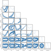 |
Fig. A.3 As Fig. A.2, but only for elliptical solutions. |
| In the text | |
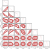 |
Fig. A.4 As Fig. A.2, but only for hyperbolic solutions. |
| In the text | |
|
Fig. C.1 Histogram of the AIC value for all walkers, separated by elliptical, hyperbolic, and hyperbolic orbits where the periastron time is before the first ALMA observation. |
| In the text | |
|
Fig. D.1 Predicted location of RW Aur B based on the elliptical (solid blue) and hyperbolic (dashed red) models, starting from July 2025, and then the July every three years until 2037. The position from the best elliptical and hyperbolic model are shown with a circles, while the contours show the 3σ scatter for each family or orbits. |
| In the text | |
|
Fig. E.1 The 12CO blueshifted emission with respect to RW Aur A is shown in panels (a) and (b), while the redshifted component is shown in (c) and (d). The beam size in the lower left corner and the scale bar in the upper right are the same for all the panels. The centers of the 2 disks are shown with black + symbols. |
| In the text | |
|
Fig. E.2 13CO Moment 0 and velocity at peak flux are shown in panels (a) and (b), while the same images for C18O are shown in panels (c) and (d). Beam sizes are shown in lower left corner, and a scale bar of 20 au is shown in the upper right corner. |
| In the text | |
Current usage metrics show cumulative count of Article Views (full-text article views including HTML views, PDF and ePub downloads, according to the available data) and Abstracts Views on Vision4Press platform.
Data correspond to usage on the plateform after 2015. The current usage metrics is available 48-96 hours after online publication and is updated daily on week days.
Initial download of the metrics may take a while.