| Issue |
A&A
Volume 691, November 2024
|
|
|---|---|---|
| Article Number | A38 | |
| Number of page(s) | 22 | |
| Section | Cosmology (including clusters of galaxies) | |
| DOI | https://doi.org/10.1051/0004-6361/202451316 | |
| Published online | 25 October 2024 | |
The glow of axion quark nugget dark matter
II. Galaxy clusters
1
Universitäts-Sternwarte, Fakultät für Physik, Ludwig-Maximilians Universität,
Scheinerstr. 1,
81679
München,
Germany
2
Max-Planck-Institut für Astrophysik,
Karl-Schwarzschild-Straße 1,
85741
Garching,
Germany
3
Department of Physics and Astronomy, University of British Columbia,
Vancouver,
V6T 1Z1,
BC,
Canada
4
Univ. Lille, CNRS, Centrale Lille,
UMR 9189 CRIStAL,
59000
Lille,
France
5
Université Paris-Saclay, CNRS, Institut d’Astrophysique Spatiale,
91405
Orsay,
France
6
Leibniz-Institut für Astrophysik (AIP),
An der Sternwarte 16,
14482
Potsdam,
Germany
★ Corresponding author; This email address is being protected from spambots. You need JavaScript enabled to view it.
Received:
1
July
2024
Accepted:
7
September
2024
Abstract
Context. The existence of axion quark nuggets is a potential consequence of the axion field, which provides a possible solution to the charge-conjugation parity violation in quantum chromodynamics. In addition to explaining the cosmological discrepancy of matter-antimatter asymmetry and a visible-to-dark-matter ratio of Ωdark/Ωvisible ≃ 5, these composite compact objects are expected to represent a potentially ubiquitous electromagnetic background radiation by interacting with ordinary baryonic matter. We conducted an in-depth analysis of axion quark nugget-baryonic matter interactions in the environment of the intracluster medium in the constrained cosmological Simulation of the LOcal Web (SLOW).
Aims. Here, we aim to provide upper limit predictions on electromagnetic counterparts of axion quark nuggets in the environment of galaxy clusters by inferring their thermal and non-thermal emission spectrum originating from axion quark nugget-cluster gas interactions.
Methods. We analyzed the emission of axion quark nuggets in a large sample of 161 simulated galaxy clusters using the SLOW simulation. These clusters are divided into a sub-sample of 150 galaxy clusters, ordered in five mass bins ranging from 0.8 to 31.7 × 10¹⁴ M⊙, along with 11 cross-identified galaxy clusters from observations. We investigated dark matter-baryonic matter interactions in galaxy clusters in their present stage at the redshift of z = 0 by assuming all dark matter consists of axion quark nuggets. The resulting electromagnetic signatures were compared to thermal Bremsstrahlung and non-thermal cosmic ray (CR) synchrotron emission in each galaxy cluster. We further investigated individual frequency bands imitating the observable range of the WMAP, Planck, Euclid, and XRISM telescopes for the most promising cross-identified galaxy clusters hosting detectable signatures of axion quark nugget emission.
Results. We observed a positive excess in the low- and high-energy frequency windows, where thermal and non-thermal axion quark nugget emission can significantly contribute to (or even outshine) the emission of the intracluster medium (ICM) in frequencies up to νT ≲ 3842.19 GHz and νT ϵ [3.97, 10.99] × 1010GHz, respectively. Emission signatures of axion quark nuggets are found to be observable if CR synchrotron emission of individual clusters is sufficiently low. The degeneracy in the parameters contributing to an emission excess makes it challenging to offer predictions with respect to pinpointing specific regions of a positive axion quark nugget excess; however, a general increase in the total galaxy cluster emission is expected based on this dark matter model. Axion quark nuggets constitute an increment of 4.80% of the total galaxy cluster emission in the low-energy regime of νT ≲ 3842.19 GHz for a selection of cross-identified galaxy clusters. We propose that the Fornax and Virgo clusters represent the most promising candidates in the search for axion quark nugget emission signatures.
Conclusions. The results from our simulations point towards the possibility of detecting an axion quark nugget excess in galaxy clusters in observations if their signatures can be sufficiently disentangled from the ICM radiation. While this model proposes a promising explanation for the composition of dark matter, with the potential to have this outcome verified by observations, we propose further changes that are aimed at refining our methods. Our ultimate goal is to identify the extracted electromagnetic counterparts of axion quark nuggets with even greater precision in the near future.
Key words: radiation mechanisms: non-thermal / radiation mechanisms: thermal / dark matter
© The Authors 2024
 Open Access article, published by EDP Sciences, under the terms of the Creative Commons Attribution License (https://creativecommons.org/licenses/by/4.0), which permits unrestricted use, distribution, and reproduction in any medium, provided the original work is properly cited.
This article is published in open access under the Subscribe to Open model. This email address is being protected from spambots. You need JavaScript enabled to view it. to support open access publication.
1 Introduction
During the Big Bang, a highly energetic environment sets the foundation for theories to emerge regarding matter and its composition. Evolved from different cosmological environments, modern theories describe a versatile zoo of dark matter models ranging from, for instance, sterile neutrinos (Dodelson & Widrow 1994; Shi & Fuller 1999), axion-like particles (Georgi et al. 1986; Masso & Toldra 1995; Masso 2003), weakly interacting massive particles (Steigman & Turner 1985), and quark nuggets that typically exhibit nuclear density (Witten 1984; Farhi & Jaffe 1984; de Rujula & Glashow 1984). In addition to the comparatively low-mass dark matter candidates, massive astrophysical compact halo objects (Alcock et al. 1993; Aubourg et al. 1993) with for instance primordial mass black holes could propose a promising alternative as well (Zel’dovich & Novikov 1967; Hawking 1971; Chapline 1975). Constraints on mass, properties, and number densities of these dark matter candidates can be made by various techniques. As for potential dark matter candidates, particle accelerators are instrumental in proposing mass boundaries for elementary particles, while gravitational wave detectors may aid in constraining the distribution of primordial black holes. A dark matter candidate is rarely observationally falsifiable by testing signatures in the electromagnetic spectrum.
Here, we present a detailed analysis of the observational feasibility ofa dark matter model that is proposed to obey properties of cold dark matter, but is still expected to be the origin of observable signatures that can be tested in a wide range of the electromagnetic spectrum, called the axion quark nugget (AQN, Zhitnitsky 2003). These nuggets are not only capable of describing generic cold dark matter features of structure formation but also provide solutions to fundamental cosmological problems. Two of the most prominent mysteries are related to (i) why the abundance of dark matter is not extraordinarily lower or larger than the visible component; and (ii) why we tend to observe more matter over antimatter and where this imbalance comes from.
This paper is structured as follows. In Sect. 2, a short overview is provided by focusing on the formation, structure, and interaction scenario of AQNs in the respective subsections. Furthermore, the foundation of interaction-resulting electromagnetic signatures is set in Sect. 3. A physical description responsible for the electromagnetic counterpart is provided in Sects. 3.1 and 3.2. The implementation method using a smoothed-particle hydrodynamics (SPH) formalism in a constrained cosmological simulation is presented in Sect. 3.3, with more details on the simulation provided in Sect. 3.5. Selection criteria and details on our underlying sample are presented in Sect. 3.6. Our results are provided in Sect. 4, followed by a discussion of our findings in Sect. 5. An outlook in conjunction with a concluding assessment is provided in Sect. 6.
2 General overview of AQNs
2.1 The formation process
In this section, we describe the key steps for the formation of these particles and refer to (Liang & Zhitnitsky 2016; Ge et al. 2017, 2018, 2019) for further details. Quantum chromodynamics (QCD) has a chiral anomaly term characterized by an axial angle θ. This angle θ is physical and observable in the standard model. When θ ≠ 0, the anomaly term induces a charge-conjugation Parity (C𝒫) violation, namely, the laws of physics do not behave in the same way under combined transformations of charge conjugation and parity. This leads to the so-called strong C𝒫 problem, since the C𝒫 violation in QCD is not observed (Abel et al. 2020). The strong C𝒫 problem can be naturally resolved when θ is considered a dynamical field so that the vacuum expectation value ⟨θ⟩ settles to zero after the QCD transition. Consequently, the dynamical field θ produces a hypothetical particle called axion1. The axion is very light and couples very weakly with ordinary matter.
In the framework of AQN, axions are produced before inflation. In this scenario, a unique physical vacuum occupies the entire Universe, and most types of topological defects [including the NDW, 1 domain walls (DWs)2] are forbidden. Only the NDW = 1 DWs, when θ interpolates in a single physical vacuum but different topological branches θ → θ + 2πn (Vilenkin & Everett 1982; Sikivie 1982), can be produced. The NDW = 1 DWs may form when the axion field starts to oscillate due to the misalignment mechanism at temperature Tosc ∼ 1 GeV. This process continues until the QCD transition Tc ∼ 170 MeV when the quark chiral condensates form. From Tosc to Tc, the axion mass effectively turns on, and the axion oscillation is underdamped. At the beginning of the oscillation Tosc, the axion field is coherent globally. A coherent nonzero θ violates the global C𝒫 symmetry and affects the DW formation. Consequently, a preferred matter or antimatter species of nuggets will be formed – it should be mentioned though, that an equal amount of nuggets would have been formed if θ = 0 at the moment of the DW formation. Only the initial sign of the coherent θ field before oscillation dictates which nugget family is preferably formed.
A small portion of the NDW = 1 DWs forms closed bubbles and acquires baryon charges from the quark-gluon plasma. Near and after the QCD transition Tc, the DWs on the bubbles can mix the axion with a tilted η′ field (the field of the η′ meson). Such a tilted substructure boosts the charge accumulation of the DW bubbles. Depending on its inherent topological charge, a bubble acquires either matter or antimatter charges during this phase. Charge accumulation terminates at Tform ∼ 41 MeV and the bubbles form quark nuggets in the form of color superconducting (CS) condensate. Due to the C𝒫 violation effect discussed earlier, more antimatter AQNs are formed compared to matter AQNs. Under the assumption of zero baryon net charge in the Universe, the observed visible-to-dark-matter-density ratio of Ωdark : Ωvisible ≃ 5:1 implies a baryon charge ratio of
 (1)
(1)
where the subscripts of B correspond to the baryon charges of antimatter AQNs, matter AQNs, and visible matter, respectively. Both, the matter- and the antimatter-AQNs serve as the dark matter component, while the remaining quarks in plasma become the visible component. Unlike conventional dark matter candidates such as weakly interacting massive particles (WIMPs) and axion, the AQN explains the observed cosmological relation Ωdark ~ Ωvisible without fine-tuning of fundamental parameters, since dark and visible matters now have the same QCD origin. In the AQN framework, freely propagating axions may exist via the misalignment mechanism (Abbott & Sikivie 1983; Dine & Fischler 1983; Preskill et al. 1983) and topological defects (Chang et al. 1998; Kawasaki et al. 2015; Fleury & Moore 2016; Klaer & Moore 2017; Gorghetto et al. 2018). However, they contribute a negligible amount to the dark sector Ωdark unless very specific fine-tuning applies (Ge et al. 2018). The conclusion (1) is unaffected.
The CS condensate in the AQN is stabilized by the excessive surface tension of the DW bubble. The binding energy in the CS phase is sufficiently large (with a gap Δ ~ 100 MeV) so that AQNs do not modify the basic elements3 of the Big Bang Nucleosynthesis (BBN) at TBBN ∼ 1 MeV, where elements of metallicity Z ≤ 3 were formed. Quark cores in the CS state are in the lowest energy state possible, and it is assumed that quarks in neutron stars obey the same state (Alford et al. 2008). AQNs remain in this stable state over cosmic time scales.
On the other hand, if the theory of AQNs holds, the asymmetry of matter to antimatter in the observable Universe can be explained by an asymmetric baryon charge separation. A coherent background field θ violates the global  symmetry at the beginning of DW bubble formation. This theory allows an equal amount of antimatter and matter, with more antimatter being hidden in composite nuggets than the ordinary one, causing it to be unobservable. These nuggets are stable over cosmic time, as the quark core is in a dense CS state. It serves as cold dark matter because these macroscopic particles exhibit a low number density due to individual masses of the order of grams (a more specific description will be addressed in the following section). In summary, the AQN model provides intriguing cosmological implications by explaining the matter-antimatter asymmetry and the similarity between dark- and visible-matter densities. This is because dark and visible matters share the same QCD ancestor.
2.2 Structure of AQNs and cosmological properties
It is important to differentiate matter families as (anti-)AQN consist of a core of (anti)quarks surrounded by positrons/electrons that make the electrosphere. The electrosphere is surrounded by the NDW = 1 axion DW. Interactions of baryonic matter with the axion DW seldom occur. The surface tension of the DW exerts a strong pressure on the quark core causing it to preserve in a CS state. To prevent the DW from collapsing further, Fermi pressure from the AQN counteracts the DW surface tension.
Parameters that describe the properties of an AQN are the baryon number B, the electric charge eQ, where Q typically corresponds to the number of positrons that depleted from an originally neutral AQN and in some scenarios the magnetization ℳ (Santillán & Sempé 2020), which will be neglected in this study for reasons of simplification. It will be shown in later sections that Q highly depends on the temperature of the surrounding gas as positrons can deplete if the conditions suffice. The lower limit on B can be observationally constrained by non-detections from IceCube with 〈B〉 > 3 × 1024 (Lawson et al. 2019). Similar limits are also obtainable from the ANtarctic Impulse Transient Antenna (ANITA) and geothermal data (Gorham 2012). B results in the AQN’s mass MAQN and size RAQN, with most recent discussion on their distribution in Raza et al. (2018); Ge et al. (2019). Since mass contributions from the electrosphere are negligible, the baryonic mass component of an AQN can be estimated as follows:
 (2)
(2)
In the state of a CS phase, we can assume the nuclear density to be ρn = 3.5 × 10¹⁴ gcm–3 (Zhitnitsky 2018) resulting in an AQN radius of
 (3)
(3)
Ionized AQNs are characterized by a charge Q, with Q being a function of TAQN . A small fraction of positrons in the electrosphere are loosely bound and in the non-relativistic Boltzmann regime (McNeil Forbes & Zhitnitsky 2008b), which rises with the internal AQNs temperature.
Throughout this paper, we fix the parameters to physically describe the structure of AQNs as B = 1025, MAQN = 16.7 g and RAQN = 2.25 × 10⁻⁵ cm. A distribution function of these parameters is not well-constrained yet and would drastically increase the complexity of the system.
2.3 Possible interaction scenarios
As pointed out in Sect. 2.2, AQNs consist of two different particle families and will therefore yield different combinations of possible interaction scenarios. Not all of the different interactions are likely to be visible and, therefore, their relevance for our study will be assessed in the following.
Antimatter AQN interaction with electrons: electrons can interact with the electrosphere made up of positrons for antimatter AQNs. These e+e– annihilations might possibly explain the 511 keV line emission coming from the galactic center (Oaknin & Zhitnitsky 2005; Zhitnitsky 2007; Forbes et al. 2010; Flambaum & Samsonov 2021) and the COMP- TEL gamma-ray photons in an energy range of 1-20 MeV (Lawson & Zhitnitsky 2008).
Antimatter AQN interaction with protons: free protons propagating through the electrosphere can collide with the antiquark core (see Fig. 1). Each collision produces an annihilation energy of 2 GeV. A major fraction (about 90%) of the annihilation energy will thermalize the quark core and transfer to the electrosphere. This heating process leads to the emission of the electrosphere in the form of thermal Bremsstrahlung. Observations that can be explained by thermal AQN emission are, for instance, the diffuse galactic microwave excess (McNeil Forbes & Zhitnitsky 2008b), the 21 cm absorption line (Lawson & Zhitnitsky 2019), and diffuse galactic UV background emission (Zhitnitsky 2022a). A minor fraction (about 10%) of annihilation energy will be emitted as a short pulse of non-thermal photons at the point of impact. Observations, such as Chandra’s diffuse kBT ≈ 8 keV emission (McNeil Forbes & Zhitnitsky 2008a) might find their nature in non-thermal AQN emission processes.
Antimatter AQN annihilation with celestial bodies: as it is discussed in detail by Liang (2022), antimatter AQNs can annihilate with more matter at the same time. Axions, residing off-shell in the DW can be emitted, when AQNs lose potential energy after annihilation processes in the core took place. To retain a minimum total energy of the system and therefore maintain the stability of the AQN, axions will be emitted to lower the DW’s mass. In addition to axions, antimatter AQNs produce electromagnetic radiation as described in (1) and (2). As a consequence, phenomena such as coronal heating, extreme ultraviolet (EUV), and X- ray emissions might be attributed to the outcomes of AQN interactions in the sun (Zhitnitsky 2017, 2018; Raza et al. 2018; Ge et al. 2020). The nature of fast radio bursts may be explained by AQNs by triggering magnetic reconnection events in magnetars as well (Van Waerbeke & Zhitnitsky 2019). Furthermore, according to Budker et al. (2022), infrasound, acoustic, and seismic waves might be the direct outcome of AQN-earth encounters. Non-inverted polarity detections by ANITA were discussed by Liang & Zhitnitsky (2022a), and short time bursts detected by the Telescope Array (TA) were analyzed by Zhitnitsky (2021b); Liang & Zhitnitsky (2022b) in the framework of AQN annihilations. Cosmic ray (CR)-like events detected by the Pierre Auger Observatory might be explained by AQNs inducing lightning strikes with subsequent direct emission (Zhitnitsky 2022b). Multi-modal events detected by Horizon-T that were discussed using AQNs by Zhitnitsky (2021a) should be distinct from conventional cosmic-ray showers.
Matter AQN interaction with antimatter: technically, one could expect the same emission processes from points (1) and (2) with matter AQNs with positrons and antiprotons. However, because of the low abundance of antimatter CRs (e.g. Hillas 2006; Blum et al. 2017) and the slightly lower abundance of matter AQNs over antimatter AQNs, it is expected that matter AQNs remain dark for most of the time and electromagnetic signals originating from matter AQNs can be neglected.
Matter AQN-antimatter AQN interaction: even though the electromagnetic outcome of matter-antimatter AQN interactions would result in an impressive electromagnetic signature, it is because of the low number density of nAQN ~ 10–29 cm–3 that this interaction scenario can be entirely neglected (see comments on this for example in Zhitnitsky 2022b). And although both of the AQNs can have an attractive influence on each other if ionized, the higher effective cross-section would not drastically increase interaction rates.
AQN-AQN interaction from same particle family: Since AQNs from the same particle family would only collide by chance with no interaction enhancement by their ionization state, collisions are expected to be even rarer than described in point (5). An electromagnetic signature would at most be visible by thermalization of a heated AQN after collision.
As we have assumed the intracluster medium (ICM) to consist of ionized hydrogen, this work will only focus on emission phenomena coming from proton-antimatter AQN interactions. Line emission from e+e– annihilation, axion emission by strong AQN emission, and AQN-AQN self-interactions will be neglected in this study as thermal and non-thermal AQN emission from proton interactions is presumed to dominate the spectrum.
With the fixed parameters describing a single AQN, we can infer the antimatter AQN’s number density by assuming the mass ratio relation from Eq. (1). According to the mass ratio relation, a fraction of 3/5 of the entire dark matter accounts for anti- AQNs. Since ionized gas in the ICM mainly consists of normal matter, the highest rate of annihilation processes – and hence visible interactions – will be expected from antimatter AQNs. One third of the total AQN mass comes from the NDW = 1 axion DW (Ge et al. 2018). Therefore – to account for the antimatter AQN number density nAQN from the total “observable” dark matter density pDM - we would further have to multiply a factor of 2/3 by excluding the DW contribution to the AQN mass. We therefore obtain an anti-AQN number density estimate of
 (4)
(4)
which typically scales in a galaxy cluster environment as nAQN ~ 10–29 cm–3. It is because of the low number density that AQNs mostly preserve cold dark matter features, provided they are in a suitable environment. However, the interactions that occur may even yield different emission processes with respect to AQNs. For the sake of simplicity, we further refer to antimatter axion quark nuggets by using the abbreviation “AQN”.
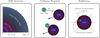 |
Fig. 1 Schematic sketch for the antimatter-AQN’s internal structure (not true to scale) with an indication of typical sizes (left panel) and the processes, which lead to the different radiation signatures (middle and right panel). The antimatter-AQN consists of a core of anti-quarks surrounded by positrons. When colliding with the ambient gas, the antimatter-AQN heats up and radiation occurs, which depends on the speed at which the collision occurs, the gas temperature and density as well as the ionization state of the gas. The right panel shows the two key emissions, namely thermal and non-thermal emissions. From an incoming proton (green, small circle), 2 GeV of energy will be available after collision with the AQN. Through annihilation, energetic quarks and gluons are produced and stream either deep within the nugget (around 90% of the 2 GeV) or toward the nugget surface (around 10% of the 2 GeV). Quarks and gluons, which remain inside, will contribute to the thermalization of the nugget. Heat will be transferred from the core to the electrosphere which cools down via thermal Bremsstrahlung emission. Quarks and gluons, which proceed to the surface without thermalization, can transfer energy to positrons and produce non-thermal emission. |
3 Methodology
3.1 Internal AQN temperatures through ambient gas interactions
The internal temperature of AQNs is influenced by annihilation processes of protons impacting a nugget with anti-quarks from the inner core. The internal temperature of a nugget can be estimated from the conservation of energy. In thermal equilibrium, if a proton is captured by an AQN, the injected energy must be equal to the radiative output. Protons can be captured more efficiently if the anti-quark nugget is ionized, but loses efficiency under certain conditions of the environment. Therefore, we have to introduce an effective cross-section σeff to model collision rates. The energy conversion efficiency during a collision depends on a proxy for the probability of quantum reflection for neutral gas called (1 – f), and the fraction of thermal photon production (1 – g) ≈ 0.9. Because of the increased Coulomb potential in an ionized gas, the quantum reflection probability  is highly suppressed, and we therefore obtain f ~ 1. The Coulomb potential causes the hydrogen ion to be trapped around an AQN until the final collision and therefore annihilation occurs. The injected energy per unit time can be estimated as
 (5)
(5)
∆E is the energy that will be released by an annihilation event of a single proton amounting up to ∆E ~ 2mpc2 ≈ 2 GeV and ∆v = |vAQN − vgas| is the relative AQN-proton speed. The radiative output is the luminosity of a nugget with radius RAQN, namely,
 (6)
(6)
If we set dE/dt = L and after re-expressing the effective cross-section  using the scaling parameter κ, we obtain the expression
 (7)
(7)
As a consequence of the internal temperature increase due to the annihilation process, the positrons in the electrosphere will be heated and emit Bremsstrahlung. In natural units, namely, c = kB = ħ = 1 and h = 2π, the total surface emissivity of an AQN is calculated by McNeil Forbes & Zhitnitsky (2008b) and given as
 (8)
(8)
Here, α is the fine-structure constant, and TAQN is the internal temperature of the AQN. After equating Eqs. (7) with (8), we can solve for TAQN and obtain
 (9)
(9)
Equation (9) can be represented more intuitively if we use galaxy cluster-typical gas densities of ngas,cluster ~ 10−3cm−3 and a relative velocity of ∆ν ~ 10−3 c:
 (10)
(10)
The numerical factor κ boosts the internal AQN temperature if the effective cross-section is larger than its geometrical cross-section. We thus use the following condition for each AQN:
 (11)
(11)
To find an expression for Reff, two important contributions have to be taken into account. First, the charge of an AQN Q, which is a proxy for the ionization stage, and second, the temperature of the surrounding plasma. In galaxy clusters, the ICM consists of highly ionized gas with temperatures of TICM ~ keV. In an entirely ionized gas, Zhitnitsky (2023) shows that the cross-section of AQNs can scale with Reff instead of RAQN, leading to a potential increase in the collision efficiency with the surrounding gas. It is important to note that geometrical radii of AQNs are of the order of RAQN ~ 0.1 µm and – given that the gas number density in galaxy clusters is of the order of ngas ~ 10−3 cm−3 – collision rates with surrounding particles can be quite low if Reff < RAQN. It is not sensible to incorporate effective radii smaller than their geometrical size, and therefore for Reff < RAQN we set Reff = RAQN. It is possible to derive Reff from the physical properties of the nugget and its environment.
In the following Zhitnitsky (2023) proposes that the potential energy of attraction for AQNs in an ionized gas scales with the thermal energy of the plasma in the environment, namely,
 (12)
(12)
with the fine-structure constant, α, the charge, Q, the proton mass, mp and proton velocity, vp. Equation (12) shows the radius at which an ionized AQN can capture protons from the gas with thermal velocities of  . What follows from this scaling relation is a capture radius which decreases for increasing gas temperatures. Zhitnitsky (2023) used the capture radius instead of the effective radius with
  . In this paper, however, we adopt the convention of using Reff instead of Rcap. After re-expressing Eq. (12), we obtain the following relation:
 (13)
(13)
It is important to note that Q is a function of TAQN. The higher TAQN, the higher the thermal motion of positrons in the electrosphere with positrons following a non-relativistic Boltzmann regime (McNeil Forbes & Zhitnitsky 2008b). If kinetic positron energies exceed the potential energy of the AQN, positrons can deplete, leading to a negative charge for AQNs. The positrons are rather weakly bound and the number of positrons Q which are likely to evaporate from the AQN can be estimated by using the mean field approximation (McNeil Forbes & Zhitnitsky 2008b) of the local density of positrons n(ɀ, TAQN) at a distance ɀ from the surface of an AQN. According to Zhitnitsky (2023), one obtains for typical TAQN in cluster environments
 (14)
(14)
 (15)
(15)
with me and units of cm from Eq. (14) being re-expressed in units of eV using natural units (i.e. c = ħ = 1 and h = 2π). Now, after using Eqs. (9), (13), (15), and κ = (Reff /RAQN)2, we find
 (16)
(16)
Equation (16) immediately implies that in a galaxy cluster environment, the majority of AQNs will be treated with κ = 1, since RAQN > Reff.
3.2 Radiation processes of AQNs
AQNs can emit both thermal and non-thermal radiation. The major fraction (1 − 𝑔) ≈ 0.9 of the annihilation energy of 2 GeV is emitted by thermal Bremsstrahlung. The remaining fraction 𝑔 ≈ 0.1 is radiated non-thermally. The total surface emissivity was already introduced in Eq. (8), which was derived as McNeil Forbes & Zhitnitsky (2008b)
 (17)
(17)
with f (x) being:
 (18)
(18)
and x = 2πν/TAQN. Majidi et al. (2024) rewrote Eq. (17) in physical units. This also changes x to  , such that we get:
 (19)
(19)
Figure 2 shows a plot of dF(v)/dν for a set of internal AQN temperatures for ν ∊ 2.42 × [108,1 020] Hz. Temperatures that fall into the cluster regime are mostly abundant in the radio and microwave bands. There is another approach (Flambaum & Samsonov 2022a, b) that assumes an emission spectrum completely different from ours. As the total flux intensity must be the same in both approaches, we do not implement this model since it is beyond the scope of this work.
In the case of non-thermal emission, McNeil Forbes & Zhitnitsky (2008a) proposed the non-thermal emission per frequency to scale with:
 (20)
(20)
with K3/5(x) being the second modified Bessel function. The critical frequency, νc = ωc/(2π) ≈ 30 keV/(2π), was approximated by McNeil Forbes & Zhitnitsky (2008a). It is important to note that νc = 30 keV/(2π), whose numerical value is set to 30 for conventional reasons, is not strictly constrained. For the expression of the synchrotron function, various approximations can be estimated by different approaches and integration methods (see for example Crusius & Schlickeiser 1986; Rybicki & Lightman 1986; Weniger & Cížek 1990; Fouka & Ouichaoui 2013, 2014; Yang & Chu 2017; Palade & Pomârjanschi 2023). For our study, we have adapted the approximation of the integrated modified Bessel function from Majidi et al. (2024):
 (21)
(21)
with C(1/3) ≈ 1.81. It is important to note that β is usually not fixed and can vary depending on the energy distribution of positrons. Additionally, the exponent depends on the emission mechanism at the nugget’s surface, which can be free-free-like emission rather than synchrotron-like, resulting in β = 0. Given the various analytical approximations and the choice of utilizing the synchrotron function to model the non-thermal spectrum requiring more physical evidence, one has to keep in mind that the non-thermal AQN spectrum is not constrained well enough to propose definite predictions. With this in mind, the non-thermal AQN emission has to be understood with caution. Nevertheless, the bolometric surface emissivity of the non-thermal component can then be calculated by substituting x with ν/νc in Eq. (21) and integrating over ν ∊ [0, ∞]. The final expression of  is derived in great detail in Majidi et al. (2024) and is directly adopted from the cited literature:
 (22)
(22)
and expressed in terms of TAQN:
 (23)
(23)
A plot of the non-thermal spectrum for typical Reff, ngas = 10−3cm−3 and ∆v = 107cm s−1 in a galaxy clusters is shown in Fig. 3. In most cases, Reff = RAQN, and when comparing this to Fig. 2 for typical AQN temperatures in galaxy clusters (TAQN ∊ [10−2, 10−1] eV), it can be seen that the non-thermal emission is expected to be a few orders of magnitude lower than the thermal emission.
In a system of multiple AQNs, a more appropriate representation of radiation is the emissivity jν, which depends on the number density of AQNs nAQN, and it is therefore crucial to evaluate individual local number densities instead of assuming a global nAQN (the denser the environment, the more emission we can expect). It is therefore important to evaluate the emissivity of each AQN tracer particle individually. With the individual emissivity, we can obtain a cluster spectrum or emission maps after summing over all individual jν. A more detailed description of how local properties in a particle simulation are inferred will be presented in Sect. 3.3. We adopted Eq. (4) for describing the number density, while we have to keep in mind that ρDM,i should be evaluated at the ith AQN tracer particle in the simulation. The emissivity is represented as
 (24)
(24)
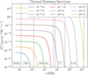 |
Fig. 2 Spectral range for thermal emission from AQNs. The magnitude and width of a thermal spectrum increase for increasing TAQN and can reach from radio to X-ray frequencies for extraordinary hot AQNs. |
3.3 Mapping AQN properties onto halo tracer particles
Cosmological simulations in the SPH formalism use tracer particles to represent environmental properties in a specific region. Depending on the resolution in our simulation, a tracer has a mass of Mpart ~ 109–1010 h−1 M⊙. In the underlying AQN model, a particle represents properties of temperature, density, and velocity relative to the environment within the region it exists in. In our analysis of the simulation, particle families are split into gas and halo tracer particles. The motion of halo tracer particles is defined only by their gravitational interactions with their surroundings. It is because of this property that halo tracer particles can serve as good tracers for AQNs in this analysis. As proposed in Eq. (10), physical properties of AQNs rely on the cluster environment – more specifically, on the underlying gas properties of the ICM. It is not trivial to find that gas properties of SPH tracer particles can be mapped onto a single halo tracer particle. Therefore, we aim to describe in greater detail how the mapping process can be numerically implemented.
Initially, the number of neighboring gas particles that can influence the AQN properties is defined to be Nneigh = 200. To reduce the computational costs, we use the package NearestNeighbors.jl (Carlsson et al. 2022) and sort particles by the k-d tree algorithm to find the nearest gas neighbors surrounding an AQN particle.
Once all the gas particles have been localized for each AQN, the relative velocities in each of the x, y, and z-coordinates to all neighboring gas particles can be calculated to infer the speed, which is then saved in an array. Depending on their distance relative to the gas particles, AQNs are characterized by different weights, 𝒲, for each neighboring gas particle. Kernel weights are usually a function of the corresponding kernel function, kK, the AQN distance to the jth gas particle, di,j, and the smoothing length, hAQN,i = max(d) if d ≠ 0 of an AQN with respect to the jth gas particle; namely, 𝒲AQN(kK, di,j, hAQN,i), and can be calculated by using the package SPHKernels.jl (Böss 2023). A 3D Wendland C2 kernel is chosen for AQNs and a 3-dimensional Wendland C4 for gas particles (see Dehnen & Aly (2012) for choosing kernels). When considering the ·th AQN particle, any arbitrary SPH property Aj of the jth gas particle can be calculated according to Dolag et al. (2008) via
 (25)
(25)
In this case, this is how 〈∆vi〉 is calculated. However, to properly infer gas properties at positions of AQN particles relative to their environment, it is crucial to define a kernel that computes weights only from the given gas HSML property and their corresponding distances to the AQN. For the gas properties, we therefore obtain the mapped gas particle SPH property onto the AQN via
 (26)
(26)
This finally gives us the following set of equations that have to be solved numerically:
 (27)
(27)
 (28)
(28)
 (29)
(29)
Here, hgas,j can be directly obtained from the HSML block of each gas particle. To ensure that numerical values do not fall below sensible SPH values, the conditions
 (30)
(30)
 (31)
(31)
are applied. For reasons of simplification, only the absolute relative velocity for each particle was taken to calculate an SPH representative for the AQN, which can be calculated via
 (32)
(32)
It is a direct consequence of this approach that 〈∆vi〉 is obtained independently of the direction of the velocity vector of a gas particle relative to the AQN. Only a single scalar is saved to describe the smoothed speed of an AQN with respect to its environment. It is therefore possible that particles are strongly weighted because of their relative distance to the AQN particle but have already passed the AQN and are moving away. This circumstance, on the other hand, is not too big of an issue, since tracer particles are representations of particle distributions, and direct collisions are therefore not desired in the setup of an SPH simulation.
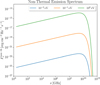 |
Fig. 3 Non-thermal AQN emission spectrum for different TAQN serving as a validation to reproduce Fig. 3 from Majidi et al. (2024). |
3.4 Additional radiation sources in simulated galaxy clusters
3.4.1 ICM Bremsstrahlung
It is important to compare the AQN emission to gas emission to infer AQN excesses and to identify potential emission windows. Amongst other sources of radiation in the X-ray continuum, Bremsstrahlung coming from the hot ICM is the most dominant emission process (Felten et al. (1969), and Sarazin (1986) for an overview). Following Sect. 3.3, two different SPH gas properties are accessible: the gas properties at each AQN position and the gas properties at each gas particle. For gas emission, the latter will be chosen, since the spatial distribution of gas particles differs from the ones of halo tracer particles. It is specifically important to analyze different regions where gas emission is more prominent and where AQN positions might differ. The X-ray emissivity jX-ray,ν in the energy band [ν0, ν1] depends on the hydrogen mass fraction, XH, the gas temperature, Tgas, the gas density, ρgas, on the gaunt factor, 𝑔(ν, Tgas), and the frequency, ν. It takes the following form:
![Mathematical equation: $\matrix{ {{j_{{\rm{X - ray}}}} = 4{C_j}g\left( {v,{T_{{\rm{gas}}}}} \right){{\left( {1 + {X_H}} \right)}^2}{{\left( {{{\mathop n\limits^ } \over {\mathop f\limits^ {m_p}}}} \right)}^2}\rho _{{\rm{gas}}}^2\left[ {{\rm{g}}{\rm{c}}{{\rm{m}}^{ - 3}}} \right]\sqrt {{T_{{\rm{gas}}}}[{\rm{keV}}]} } \hfill \cr { \times \left( {\exp \left( { - {{h{v_0}[{\rm{keV}}]} \over {{T_{{\rm{gas}}}}[{\rm{keV}}]}}} \right) - \exp \left( { - {{h{v_1}[{\rm{keV}}]} \over {{T_{{\rm{gas}}}}[{\rm{keV}}]}}} \right)} \right){\rm{erg}}{\rm{c}}{{\rm{m}}^{ - 3}}{{\rm{s}}^{ - 1}},} \hfill \cr } $](/articles/aa/full_html/2024/11/aa51316-24/aa51316-24-eq40.png) (33)
(33)
with
 (34)
(34)
and
 (35)
(35)
where XH = 0.76 is a parameter of the simulation, and Cj = 2.42 × 10⁻²⁴ is a numerical factor provided by Bartelmann & Steinmetz (1996). Since a detailed comparison of the AQN and gas spectra requires the emissivity per unit frequency and Eq. (33) only provides the emissivity in an integrated form, we must take the derivative per frequency bin to obtain the units of erg cm−3Hz−1 s−1. In the numerical implementation, a frequency array of 1000 elements was defined in the frequency range of ν ∊ [10−5, 108]/(2π)eV given in log-space. Each consecutive element has an increased factor of a = νi+1/νi, which is constant for any i. For the factor a, we can therefore choose i = 0 for simplification, namely, the first element in the frequency array. Then, ∆νi = avi − νi is then the ith frequency band, providing a sufficient approximation for the derivation with:
 (36)
(36)
3.4.2 Estimating the synchrotron emission of the ICM
There are various sources of synchrotron emission within galaxy clusters. For a detailed, recent review on radio emission from galaxy clusters, see (van Weeren et al. 2019). Most importantly for our work, some clusters show large-scale volume filling radio emission that roughly follows the distribution of the ICM, so-called giant radio halos. Their exact nature is still under debate and theoretical models involve turbulent re-acceleration processes and/or secondary electrons from hadronic interactions. Other sources like peripheral radio emissions, so-called relics that are related to shocks or radio emission related to individual galaxies, or active galactic nuclei and their jets will be neglected for this first study. Given the large uncertainty involved when directly modeling the radio emission from first principles from our simulation (see discussion in Böss et al. 2023), we decided to follow to more conservative approach to producing the possible synchrotron signal from the ICM when comparing to the predicted AQN signal. Here, we made use of the fact that observations of a large sample of galaxy clusters suggest that, compared to the Coma galaxy cluster, other clusters typically show less or even no diffuse radio emission (Hanisch 1982; Cuciti et al. 2021). In addition, due to the quasi-near linear correlation observed between the radio signal and the Sunyaev-Zeldovich effect (Planck Collaboration Int. X 2013) we can directly relate the monochromatic radio emissivity to the pressure of the ICM. The radio halo of Coma is also observed at various frequencies so that an overall spectrum can be used (Thierbach et al. 2003). Making use of having a very good counterpart of Coma in our constrained simulation (Dolag et al. 2023; Hernández-Martínez et al. 2024) we, therefore, assume a scaling of the pressure within the simulation with the radio emissivity at 352 MHz, which reproduces the scaling presented in Planck Collaboration Int. X (2013) and modified at different frequencies to reproduce the spectrum measured in Thierbach et al. (2003). This reproduces the observed scaling relation between mass and radio power at 1.4 GHz very well (Cuciti et al. 2021); although with this approach, every cluster shows a giant radio halo. Thus, it gives an upper limit of the expected synchrotron emission from the ICM in the simulations.
3.5 The constrained simulation of the local universe “SLOW”
The underlying simulation is a constrained cosmological simulation of the local universe, called Simulating the LOcal Web (SLOW, Dolag et al. 2023). Derived from the CosmicFlows-2 catalog (Tully et al. 2013), the peculiar velocity field can help to constrain initial conditions for a simulation of our local universe, when tracing back the trajectories up to a defined redshift. Tracers, such as the velocity and density fields, are direct proxies for the underlying gravitational fields which are important for the initial conditions of the simulation. This study uses the constrained cosmological simulated simulation, covering a volume of (500 h−1Mpc)3 and including 30723 gas and dark matter particles. It assumes a cosmology based on Planck measurements (Planck Collaboration XVI 2014), with a Hubble constant H0 = 67.77 km s−1 Mpc−1, a total matter density ΩM = 0.307115, a cosmological constant ΩΛ = 0.692885, a baryon fraction ΩB = 0.0480217, a normalization of the power spectrum σ8 = 0.829 and a slope of the primordial fluctuation spectra n = 0.961 as described in Dolag et al. (2023).
3.6 The sample
In this work, we tested the spectral emission of AQN quantitatively for a large sample and qualitatively for a small sample. A large sample of 150 galaxy clusters (which we call “sample 𝒜”) ordered in five corresponding mass bins was used to test scaling relations and mass dependencies for the search of emission excesses in the spectra. Each mass bin was defined to contain 30 galaxy clusters with bin sizes of Mvir, 1 ∊ [0.8, 0.9] × 1014M⊙, Mvir, 2 ∊ [1.1, 2.0] × 1014M⊙, Mvir,1 ∊ [4.0, 5.0] × 1014M⊙, Mvir,1 ∊ [7.0, 7.9] × 1014M⊙ and Mvir,1 ∊ [10.7, 31.7] × 1014M⊙. Mass bins were arbitrarily chosen to maintain a relatively equal mass distribution and conserve a well-distributed population of virial masses. The lowest mass range was chosen to be 0.8 × 10¹⁴M⊙ since it becomes tricky at lower masses to separate galaxy clusters from galaxy groups. As an upper mass range, the 31.7 × 10¹⁴M⊙ were obtained by taking the most massive galaxy clusters above the boundary of 1014M⊙. We used the subfind algorithm (Springel et al. 2001; Dolag et al. 2009) implemented into the GadgetI0.jl package (Böss & Valenzuela 2023) to receive the necessary halo IDs to read out the halo and gas tracer particles within a certain box.
“Sample ℬ” consists of 11 out of 45 cross-identified galaxy clusters (Hernández-Martínez et al. 2024) that resemble digital twins to their real counterparts, which was then utilized to identify the most promising galaxy cluster candidates that exhibit AQN signatures. According to Hernández-Martínez et al. (2024), galaxy clusters from observations were cross-identified with simulated galaxy clusters by comparing their mass, X-ray luminosity, temperature, and Compton-y signal. A probability of cross-identification can be established by measuring the probability of obtaining each cross-match in a random, unconstrained simulation. By computing the significance, the authors could assess how well the cross-identified clusters are associated with each other. The most massive galaxy cluster from the digital twin-sample is Coma (Mvir = 18.82 × 10¹⁴ M⊙) and the least massive is Fornax (Mvir = 0.61 × 10¹⁴ M⊙).
Galaxy clusters from both sample 𝒜 and sample ℬ were read out from a sphere of radius r = b × rvir, where b = 1.5 is a chosen multiplier used to extend the sphere.
4 Results
4.1 Environmental impact onto physical properties of AQNs
The histograms presented in Fig. 4 show the distribution of TAQN, Δv, nAQN, Reff, ngas, and Tgas, respectively. Out of the distributions of all 150 galaxy clusters, the median distribution in each mass bin (namely for 30 galaxy clusters each) was taken and plotted. It can be seen that the larger the range gets, all properties start to show a relatively wider distribution with fewer outliers. Since the cluster mass directly scales with the particle numbers, a general trend of increased total counts can be seen in all histograms; however it is interesting to see how the shape of the histograms changes for increasing mass bins.
Relative velocity: in the Δv-histogram, most of the particles are distributed towards Δv ~ 108cms−1 ~ 0.3%c. Intriguingly, an additional low-velocity population component of Δv ≲ 106cms−1 seems to be present, especially in massive galaxy clusters. A Δv peak shift towards higher velocities for larger cluster masses can also be observed.
Internal AQN temperature: the TAQN-histogram is heavily weighted for values of TAQN ∈ [10−2,10−1]eV and occasionally high TAQN ≳ 1 eV can be possible for massive clusters. Peaks in the distribution shift from approximately 4 × 10⁻² eV to 6 × 10⁻² eV for increasing cluster masses. Here, Δv is likely to play the dominating factor (as discussed before). On the low TAQN -side, fewer counts are caused by non-optimal combinations of Δv, ngas and Tgas. The higher TAQN -side is limited by an increasing amount of high counts of high Tgas .
Effective AQN radius: the Reff-histogram directly shows that most of the Reff are set to RAQN = 2.25 × 10⁻⁵ cm, since κ = 1 in most environments. Depending on the cluster mass, the general shape of the Reff distribution does not drastically change.
AQN number density: following Equation (4), values in the nAQN -histogram are generally low, since AQNs are large and massive compared to elementary particles. Therefore, a smaller abundance of AQN is required, which results in low nAQN.
Gas number density: ngas shows a reasonable distribution with a heavier weight in number densities of ngas < 10−3cm−3 because of the extended readout-radius of 1.5 rvir.
Gas temperature: For increasing Mvir in galaxy clusters the peak in the Tgas-histograms shifts to larger values. Higher gas temperatures for heavier galaxy clusters can be expected due to a steeper potential that in return attracts more substructures. A constant infall of new galaxies continuously heats the ICM and provides a general increase in Tgas (see Sarazin 1986, for a review).
A better understanding of the spatial distribution of AQN properties in galaxy clusters can be obtained when considering their radial profiles. Figure 5 shows how Δv, TAQN, and Reff, mapped onto the position of AQNs scale with increasing distances from the cluster’s center of mass. Radial profiles were taken from each galaxy cluster in sample 𝒜 and the median radial profile was taken for each mass bin. SPH properties were inferred according to the proposed methodology in Sect. 3.3.
Relative velocity: An interesting outcome of the radial Δv profiles is that for the most massive galaxy clusters, the profile increases towards normalized distances of r/rvir ~ 0.2 and decreases at larger distances. All mass bins show relatively flat radial profiles until r/rvir ~ 0.1.
Effective AQN radius: Reff represents an intriguing property of AQNs since (due to the high ICM temperature in the central regions) the gas properties do not permit effective radii to be larger than RAQN . At larger distances, individual regional properties enable small increases in Reff that highly depend on the degenerate AQN properties present in the surrounding gas. Single substructures might be capable of obtaining large effective radii, and it is subject to Sect. 4.3 to identify these regions in spatially resolved maps of individual galaxy clusters to properly infer their physical properties. It is important to note that a slight trend of increasing Reff can already be observed at r ≤ 1.5 rvir. Even though the increase is almost negligible with a maximum increase of Reff hosted by the lowest cluster mass bin of ΔReff ≃ 3 × 10⁻⁷ cm (namely, an increase of ~1.3%), the phenomenon of higher Reff in the peripheries becomes more significant the further the distance is. This is a feature of the underlying AQN model that was anticipated for this paper, since AQNs are expected to be surrounded by a fully ionized gas. In regions of r ≫ 1.5 rvir, smaller Tgas values consequently yield large Reff, as ionized particles can be captured over larger distances if the thermal motion of the ions is sufficiently low. This will lead to a runaway effect for increasing Reff that is not physically meaningful. It is, therefore, crucial to constrain the sample to galaxy cluster regions with an extent of approximately rmax ~ 1.5 rvir at maximum for the underlying AQN model.
Internal AQN temperature: TAQN are most likely increasing for different masses with higher Δv. For larger radii and in all mass bins, TAQN seems to converge towards a single radially normalized value. Given the underlying AQN model, it is assumed that TAQN will artificially rise for radii r ≫ 1.5 rvir, because Reff → ∞ for Tgas → 0 K. Moreover, this means that at a certain relative distance, TAQN , will mainly be influenced by the properties of filaments and voids.
4.2 Spectral energy distributions
A spectral energy distribution can be obtained by using Eqs. (19), (23), and (33) for thermal and non-thermal AQN emission, and thermal Bremsstrahlung emission from the ICM, respectively. For synchrotron emission, we followed the steps described in Sect. 3.4.2. We note that we have to apply Eqs. (24)–(19), and Eq. (23), to obtain an emissivity in units of erg cm−3Hz−1s−1.
The emissivity is then calculated for each particle in each frequency in a range of ν ∈ [10−5,108]/(2π)eV with a spectral resolution of 103 bins for AQN and gas. For the CR synchrotron emission, frequency ranges of νsynch ∈ [10−5,10−2]/(2π) eV were chosen in a spectral resolution of 100 bins. Figure 6 displays the spectral energy distribution of the five mass bins from sample 𝒜: here, the median for each frequency in each mass bin was taken out of the 30 respective galaxy clusters. AQN thermal emission, non-thermal emission, ICM Bremsstrahlung, and CR synchrotron emission are represented by solid, dash-dot-dotted, dashed, and dash-dotted lines, respectively.
It is noticeable that higher cluster masses result in an increment of the general spectral energy. In this figure, our attention is drawn towards the regions where both of the AQN emission become comparable to the ICM Bremsstrahlung emission in the low- and high-energy regimes, as it is possible to obtain small frequency windows where AQN emission would overtake the ICM Bremsstrahlung. In the low-energy regime of νlow ≲ 10−3eV, AQN and ICM emission roughly increase equally for higher Mvir. This opens the possibility that thermal AQN radiation has the potential to outshine ICM Bremsstrahlung independently of cluster masses. The fact that AQNs can deliver a Bremsstrahlung intensity similar to hot X- ray gas in the radio regime is particularly interesting since in contrast to Tgas, TAQN is not as strictly related to ngas, which highly depends on the equation of state and the equilibrium condition.
On the other hand, we would like to point out that the spectrum was extended towards minimum frequencies of νmin = 10−5/(2π) eV to provide a low-frequency coverage by the synchrotron emission. For AQNs, however, it can become challenging to provide a physically meaningful interpretation for frequencies lower than νmin, because of the finite size effect (see McNeil Forbes & Zhitnitsky 2008b). Here, the plane wave approximation breaks down, as the positron wavelength becomes comparable to the size of the nugget.
This becomes a bit trickier when comparing non-thermal AQN emission to the high energy Bremsstrahlung regime in frequencies of νhigh ≳ 10 keV. Non-thermal AQN emission will increment not as strongly as X-ray emission of the hot cluster gas. Since  (see Eq. (33)) and Tgas increases with Mvir (see Fig. 4), jX-ray,ν will especially increase drastically for increasing Mvir in the high energy regime, leading to the circumstance that non-thermal AQN is expected to only be visible in sufficiently low cluster masses.
The contribution in synchrotron emission in Fig. 6 is increasing for higher Mvir because of the Compton-y parameter. Synchrotron emission is likely to interfere with the thermal AQN emission, especially in the regions where thermal AQN emission would dominate the ICM Bremsstrahlung emission. It is therefore worth noting that one has to account for synchrotron emission and ICM Bremsstrahlung in the low-energy regime when searching for an optimal frequency window for thermal AQN emission.
In the following, we focus on the promising frequency bands where AQN emission is expected to dominate. First, to measure how strongly AQN emission outshines the background emission a metric has to be defined that includes the frequency and the magnitude of the increment in emission. Depending on the mass and other physical properties of the galaxy cluster, thermal and non-thermal AQN emission will distinctively be higher or lower in individual frequencies for different galaxy clusters. Therefore, a transition frequency νT has to be defined, where the absolute summed emissivity of all AQN tracer particles per cluster per frequency (jAQN,ν) transitions from higher to lower values compared to the thermal gas emission. From a minimum frequency νmin to the transition frequency all background emission sources (including synchrotron emission) will be integrated. In the simulation, the numerical integration is conducted by applying the trapezoidal rule which is implemented in the NumericalIntegration.jl package4.
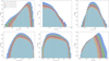 |
Fig. 4 Histograms of physical properties relevant to the AQN emission. Median values were taken for each mass bin, i.e. for 30 galaxy clusters, respectively. |
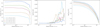 |
Fig. 5 Radial profiles of Δv, Reff, and TAQN mapped onto AQN tracer particles. The median radial profile was taken for each mass bin (i.e. 30 galaxy clusters each) and compared to other mass bins in a region of r ∈ [0,1.5] rvir. |
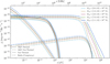 |
Fig. 6 Median cluster spectra with lines for each mass bin out of sample 𝒜 over a frequency range of ν ∈ [10−5,108]/(2π)eV. The solid, dash-dot-dotted, dashed, and dash-dotted lines represent AQN thermal emission, non-thermal emission, ICM Bremsstrahlung, and synchrotron emission, respectively. |
4.2.1 Low-frequency regime
For the low-energy regime, we define νmin as the lowest possible frequency that was used to calculate the spectra, namely, νmin = 10−5/(2π)eV because of the finite size effect of AQNs. After integration from νmin to νT, all background sources will be summed to represent a total galaxy cluster emission. The integrated spectral ratio of AQNs  significantly contributing to the background emission can be calculated as
 (37)
(37)
and
 (38)
(38)
In the following analysis,  was determined in both the low- and high-energy regimes for sample 𝒜 and sample ℬ. After applying the condition that thermal AQN emission must exceed thermal gas emission at frequencies below νT, approximately 40.99% of all galaxy clusters combined from sample 𝒜 and sample ℬ exhibit stronger AQN emission compared to the thermal background gas emission from νmin to νT.
Using this subset of galaxy clusters and applying Eq. (38), produces Fig. 7, which displays the integrated spectral ratio as a function of the transition frequency for both frequency windows where AQN emission exhibits an excess. On the left side of the figure, the thermal regime of the AQNs dominates; whereas on the right side, at high-energy frequencies, the non-thermal AQN regime dominates. An important outcome is that galaxy clusters with relatively low Mvir are still capable of reaching high  and follow relatively well-constrained tangents indicated by the colormap for different cluster masses.
It is important to find out how cross-identified galaxy clusters populate in this relation to identify promising real-world cluster candidates. Therefore, it is shown in Fig. 7 how sample ℬ is distributed in the  diagram. It can be seen in the low-energy regime that Fornax and Virgo appear to be the best candidates for the strongest AQN emission offset for the background gas emission while extending to the highest νT. Even though it is the most massive galaxy cluster in sample ℬ, the Coma cluster does not meet the condition to exhibit stronger AQN emission compared to the background emission in the energy window from νmin to νT, and is therefore not displayed in Fig. 7. Furthermore, even if synchrotron emission is excluded in Eq. (37), AQN emission does not dominate the background emission at any frequency for Coma. For a comparison of how AQN emission from other crossidentified galaxy clusters performs with and without synchrotron emission included in the background emission, see Table 1.
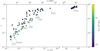 |
Fig. 7 Transition frequency-integrated ratio-relation, color-coded by Mvir with frequency ranges of positive AQN contributions. The low-energy frequency range shows in which the thermal AQN emission dominates. Low cluster masses tend to reside on a tangent, slightly offset towards higher values. The high-energy frequency range shows in which the nonthermal AQN emission dominates. Only AQN emission, originating from the lowest Mvir shows an excess over the thermal gas emission in the high-energy regime. We removed one cluster from the plot where for numerical reasons we could not compute νT and the associated |

Cross-identified galaxy clusters with physical properties from the simulation and their ability to show AQN signatures with and without synchrotron radiation in the background at a transition frequency νT in the low-energy regime.
4.2.2 High-frequency regime
Since non-thermal AQN emission is expected to show two intersections in the high energy regime, one has to define νmin to be the first transition frequency where jAQN,nonthermal,ν > jbackground,ν and νT is again where jAQN,nonthermal,ν < jbackground,ν with the condition that νmin < νT. Non-thermal AQN emission causing an excess over the background emission in the high energy regime is mostly dictated by the individual X-ray brightness of a galaxy cluster (see Fig. 6).
It can be seen on the right-hand side of the broken axis in Fig. 7 that only a small fraction of galaxy clusters could potentially dominate background gas emission with AQN emission. When applying the conditions to determine an excess in the high energy regime by AQNs, 9.32%, namely, a total number of 15 out of both samples was identified. Figure A.1 depicts the frequency window in which thermal gas emission is expected to intersect with the non-thermal AQN emission. In this image, dashed lines represent the Bremsstrahlung emission from the ICM and dash-dot-dotted lines are the non-thermal AQN emission. If there is an excess occurring, the signature is only very subtle and many low-mass galaxy clusters are still too bright in X-rays to permit a window for non-thermal AQN emission to dominate. When comparing both regimes in Fig. 7, it can be seen that in the high-energy regime, an AQN excess can only be visible for low cluster masses, which then results in a dimmer gas emission. Galaxy clusters in a higher dynamical state of dark matter particles to the surrounding gas particles could additionally positively contribute to a non-thermal AQN-excess, since jAQN,nonthermal,ν~nAQNngas∆v.
It should be noted that the non-thermal emission model is not as robust as the thermal emission model of the AQNs. In future studies, the exponent of 1/3 in Eqs. (22) and (23) for the frequency, will most likely be replaced by a free parameter β, which would be allowed to remain adaptive. The exponent of 1/3 is an approximate solution to solve the synchrotron function. It is crucial to note that particular solutions for the synchrotron function to model the non-thermal spectrum have to be motivated in greater detail and new precise models should aim for a more detailed physical implementation. In addition, the critical frequency as proposed in Sect. 3.2 is set to 30 keV by convention and should be understood in an “order of magnitude estimate” (McNeil Forbes & Zhitnitsky 2008a). To provide improved estimates, a refined theory of the non-thermal physics in the structure of AQNs is desired. The current model utilizes an approximate treatment in the mean-field of the Maxwell equations. Therefore, it is not yet possible to discard the possibility of detecting AQN signatures in the high energy regime immediately and a final conclusion shall be made once a better non-thermal AQN model is developed.
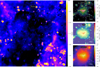 |
Fig. 8 Ratio map expressed in |

4.3 Cluster maps
It is important to note that one loses information when only considering spectral features. Since AQNs spatially follows the halo distribution, positions of dark matter with respect to gas might slightly differ from each other. Extremely low emissions do not contribute to the spectrum, because jν was summed over all particles in the corresponding frequency bin, so spatial regions of low emission are not resolved in a spectrum. It is especially important for the gas emission to identify regions of low emissivity where AQN emission would be proficient to outshine thermal gas emission. It can even be possible to find an AQN excess in small regions in spatially resolved maps where one did not expect an excess only by considering the spectrum (see, for example, the Coma cluster presented in Fig. 8). On the other hand, it is not possible to look for excess features in all 161 galaxy clusters by finding their individual optimal region where AQN features dominate over the background emission when scanning through a spectral resolution of 1000 frequency bins. We, therefore, stick to the methodology presented in Eq. (37) to analyze cluster regions, where AQN radiation certainly dominates in the spectrum by inferring the emission offset and only consider promising candidates of cross-identified galaxy clusters. Note that for simplicity the maps for all clusters are done in super- galactic x/y coordinates and not rotated to match a real observer in the local universe.
Given this reasoning, in this section, the SPH maps of gas and AQNs are represented using their most contributing physical properties and fluxes integrated over an adaptive best possible frequency range. Figures 9 and 10 display the Fornax and Virgo clusters in a selection of relevant properties.
Relative pressure maps were obtained by generating SPH maps by utilizing the ideal gas relation, pgas ~ ngas Tgas. Hence, the product of ngas and Tgas will represent the scaling of the pressure in the gas particles, and SPH maps were constructed this way. With the obtained pressure map, a Gaussian filter was applied to the projected bitmap of the galaxy cluster with σ = 5 in the Gaussian kernel. The relative pressure change is therefore obtained via
 (39)
(39)
In Fornax (see Fig. 9), fewer filamentary structures with strong emission are visible in thermal AQN emission compared to thermal gas emission because dark matter is not affected by environmental friction effects that would perturb the particle distribution. In the map depicting  , the strongest contributions originate from a larger infalling substructure, which is visible in the effective radius map as well. The
  specifically shows the presence of the glowing axion quark nugget component, which seems to show strong emissions in regions of the ICM.
Prominent regions of Reff > RAQN are only possible if the gas environment provides the necessary parameter combination. Compared to other cross-identified galaxy clusters, it is rather rare to see large regions with high Reff values. The effective radius increments with increasing ngas and ∆v and decrements for increasing Tgas. Tgas scales with the largest exponent and therefore shows the strongest influence on Reff with especially high gas temperatures in the central regions. Fornax is a relatively small cluster with a comparable low thermal gas emission coming from a low Tgas. Reff can therefore reach values of Reff > RAQN in central regions, too. However, when comparing Reff maps in Fornax to Virgo and Coma, we can see that Reff > RAQN values are more likely to be found in the peripheries of galaxy clusters.
An intriguing physical property is that regions of Reff > 10−4 cm are typically not abundant in relative velocity maps, and it is especially in these regions where ∆v seem to be lower compared to their nearest surroundings. Following  (cf. Eq. (16)), gas overdensities in conjunction with low Tgas yield higher Reff. In the case of Fornax, the prominent Reff > RAQN-region is too close to the cluster center and will therefore be hotter than in the outskirts. In this case, ngas would be the only free parameter that could directly influence Reff.
Regions of high TAQN do not necessarily follow the nAQN distribution, since TAQN is also influenced by the surrounding gas. Shocked regions are not significantly embedded in the AQN emission map and vice versa. A further interesting feature is that the AQN emission does not seem to show a significantly stronger abundance at extended regions. This is not trivial since dark matter particles do not suffer from friction and do not interact other than with gravity in the simulation. Therefore, it would have been sensible to expect additional emission contributions in the periphery of Fornax that are not strongly present in the gas emission maps.
The Virgo cluster (see Fig. 10) differs strongly from Fornax as it is more massive, hotter, and in a more relaxed state. No signs of a current major merger are visible in the relative pressure maps (other than visible in Fornax with its prominent northern bow shock). And yet, both of these clusters independently show the strongest AQN excess. It is not obvious that shock features are no tracers for AQN emission as shocked regions are always accompanied by significant offsets in thermodynamic properties (e.g., density or temperature). Even though it was expected that at least shocked regions would play a diminishing or reinforcing role on the AQN emission, this could not be directly confirmed for any of the galaxy clusters in this study. Consequently, shock maps of other cross-identified galaxy clusters do not show any signs of shock signatures in the AQN maps either.
In the  -map of the Virgo cluster, we can see that substructures show a mix of stronger and weaker contributions from the AQN emission to the ambient background emission. High ∆v in the outskirts of Virgo have an impact on larger values of
  in the peripheries. This direct influence, however, is not obvious in the case of Fornax. In the Virgo cluster, the strongest contribution of
  seems to originate from the regions of the ICM instead of the infalling substructures. This suggests we ought to look for AQN signatures where no galaxies are located when searching for signatures outside the center of the galaxy cluster.
In both clusters, we can see that high ∆v can also be reached in the clusters’ peripheries. The distribution of strong ∆v appears to be anisotropic and AQN emission does not necessarily follow the distribution of high relative velocities on large scales.
To learn how AQN signatures evolve in bands of higher energies, individual energy ranges of four different instruments were taken. AQN and gas emission were integrated within the respective energy ranges and AQN emission was superimposed by its thermal and non-thermal components. For the sake of versatile energy coverage, the instruments Wilkinson Microwave Anisotropy Probe (WMAP; Bennett et al. 2013), Planck (Tauber et al. 2010), Euclid (Laureijs et al. 2011), and the X-Ray Imaging and Spectroscopy Mission (XRISM; Mori et al. 2022) were considered. Table 2 shows the corresponding maximum energy range with upper and lower limits denoted by νmin and νmax for each instrument in units of GHz.
In the following, the two most promising galaxy clusters, determined by the top figure in Fig. 7 were selected for a multiband analysis. Figures 11 and 12 show the gas and AQN emission with the corresponding ratio image in the selected bands. To compare how the brightness of the emission evolves, all frames in their corresponding emission feature share the same colorbar limits.
While the gas emission shows a continuing brightening for increasing band energies, the AQN signatures show a signiflcant decrease in brightness in the Euclid band. This decrement originates from the spectral feature that thermal AQN emission transitions into the non-thermal regime. Euclid operates in the energy range, where the thermal emission experiences its cutoff (cf. Fig. 6). Even though AQN signatures show a re-brightening once the non-thermal regime takes over, AQN emission cannot compete with the thermal gas emission in the X-ray regime. It is evident in the ratio-images that AQN emission would only be able to dominate in the low-energy regime. A re-brightening in the higher energy bands is only visible in infalling substructures, however, the ambient glow is no longer as abundant.
We may conclude, thus, that Euclid and XRISM are the least promising instruments for a potential AQN signature detection as the thermal gas emission dominates over the AQN emission in this energy range. Furthermore, WMAP and Planck, exhibit AQN signatures in the ratio-images, even when combining thermal gas emission with synchrotron emission.
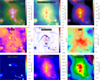 |
Fig. 9 Cross-identified Fornax cluster represented in different relevant properties. |
 |
Fig. 10 Cross-identified Virgo cluster represented in different relevant properties. |
Band-passes for WMAP (Bennett et al. 2013), Planck (Tauber et al. 2010), Euclid (Laureijs et al. 2011) and XRISM (Mori et al. 2022) in units of GHz.
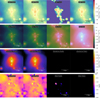 |
Fig. 11 Fornax cluster AQN, gas, and synchrotron emission generated from WMAP, Planck, Euclid, and XRISM energy ranges. Synchrotron emission is predominantly abundant in WMAP and Planck bands. Thermal gas emission shows the most significant contribution to the background emission in the Euclid and XRISM energy bands. |
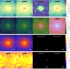 |
Fig. 12 Virgo cluster AQN, gas, and synchrotron emission generated from WMAP, Planck, Euclid, and XRISM energy ranges. Synchrotron emission is predominantly abundant in WMAP and Planck bands. Thermal gas emission shows the most significant contribution to the background emission in Euclid and XRISM energy bands. |
4.4 Observational feasibility of promising cluster candidates
It is clear from the discussion in Sect. 4.3 that the spatial features of strong AQN signatures are hard to identify and differ from cluster to cluster and their dynamical states. Even though AQN emission excess is abundant in galaxy clusters, it becomes challenging to pinpoint regions of clusters that are expected to be the most promising.
In observations, galaxy cluster emissions are typically analyzed by radial profiles in a given frequency band. This approach enables the identification of important spatial features that are dependent on distance and the corresponding frequency band. In this section, the radial profiles are shown for the cross-identified galaxy clusters that show an excess signature of thermal AQN emission integrated over their individual frequency bands from νmin to νT. Radial profiles in 50 bins were taken for each emission property and a final radial profile was calculated after summing the AQN, gas, and synchrotron maps.
Figure A.2 shows how the  evolves for the cross-identified galaxy clusters over a radius of r ∊ [10-2,1.5] rvir. An interesting feature in the radial profiles is that galaxy clusters exhibiting high
  in Fig. 7 also show high ratios in their central regions. In comparison to the remaining cross-identified galaxy clusters, Fornax and Virgo stand out in Fig. A.2.
In all radial profiles, the most significant contribution of thermal AQN emission comes from the peripheral regions, where thermal gas and synchrotron emissions have sufficiently decreased.
5 Discussion
Numerical analysis of AQNs in galaxy clusters in a cosmological simulation has shown that direct signatures of this new dark matter model are possible, but can be challenging to pinpoint. The spatial distributions of significant AQN emission contributions depend on factors, like the dynamical cluster state and thermal AQN emission is spectrally superimposed with non-thermal synchrotron and thermal gas emission.
Given that the spectral AQN signature is not exactly Bremsstrahlung and differs from synchrotron, component separation (where templates are used and spectral signatures help disentangle sources of emission) could be a reasonable strategy to look for weak AQN contributions. Multifrequency data would especially improve this approach (see Majidi et al. 2024 for a discussion).
In Sect. 2.3, tracers of AQN signatures, and further unexplained observational phenomena were pointed out and analyzed by various studies. The study by Lawson & Zhitnitsky (2019) proposed that thermal AQN emission might be responsible for a stronger absorption feature in the 21 cm line at a redshift of z = 17 during the early universe. Clusters of galaxies have not formed at this time yet and early protoclusters – observationally confirmed to be progenitors of present-day galaxy clusters – are detected at z ~ 6–7 (Harikane etal. 2019). Cosmological, hydro-dynamical simulations suggest that a hot ICM is already present at z = 4.3, at least within the core of such a protocluster (Remus et al. 2023). We therefore cannot assume the same conditions for the AQN increment which was obtained in the framework of this paper. However, it is worth mentioning that protoclusters at z ~ 7 could be capable of influencing the radio background if the AQN signal would be similarly significant as in galaxy clusters at present time. An increment in AQN emission was concluded in Majidi et al. (2024) after constructing a light cone to a redshift of z = 5.4 using the Magneticum5 simulation (Dolag et al. 2016). The sum of the AQN emission increment in the radial profiles from the cross-identified galaxy clusters of our work at z = 0 can be attributed to  thermal AQN emission.
It is, however, important to mention that early clusters possess different physical properties (Chiang et al. 2013; Overzier 2016), which would likely yield different AQN signatures. Results from this study only provided information of AQN signatures from cluster properties at z = 0. It would be sensible to implement AQN features already in snapshots at higher redshift and develop a dynamical AQN-treatment, to grasp a full evolution of AQN signatures from early to present-time galaxy clusters that could contribute to the background radio emission.
The study by Zhitnitsky (2022a) analyzed the diffuse galactic UV radiation and suggested that hot AQNs with TAQN ~ 5 eV could reproduce such observations – however since our study focuses on scales of galaxy clusters and not galactic scales, we cannot verify these predictions. The same argumentation is applied to the proposal to the contribution of Chandra’s diffuse 8 keV emission by AQNs (McNeil Forbes & Zhitnitsky 2008a). However, it is worth commenting that in a galaxy cluster, it is rather unlikely to find AQNs with temperatures of 5 eV because of the suppression of capturing protons in the hot ICM.
Galactic environments differ strongly from galaxy cluster environments with different Tgas, ngas, nDM, and Δv as the interstellar medium is cooler and denser than the ICM. In addition, galaxies exhibit a significantly lower gas emission, and especially non-thermal AQN emission in the high energy regime might indeed be capable of dominating highly energetic galactic background emission.
It is not possible to comment predictions on the 511 keV, as predicted by Oaknin & Zhitnitsky (2005); Zhitnitsky (2007); Forbes et al. (2010); Flambaum & Samsonov (2021) as we did not consider e+e- annihilation lines in our approach.
In Sect. 4.3, AQN emission was studied for different instruments in their corresponding bands. While this paper focused on AQN properties in galaxy cluster environments rather than properties within the Milky Way, a direct comparison to McNeil Forbes & Zhitnitsky (2008b) cannot be conducted. Nevertheless, it is striking to observe the abundance of AQN signatures in the WMAP maps depicted in Figs. 11 and 12. AQN signatures in the WMAP band-pass can be identified even after including synchrotron background emission. While it is important to interpret the results with caution given the significant differences between cluster and galactic properties, the possibility of an excess in microwaves in the galactic core due to AQN emission may not be entirely unfounded.
6 Conclusions
We studied the glow of axion quark nugget dark matter as signatures in a large sample of 161 simulated galaxy clusters using the constrained cosmological simulation of the local universe, SLOW. We provide lower-limit predictions on electromagnetic counterparts of AQNs in the environment of galaxy clusters by inferring their thermal and non-thermal emission spectrum originating from axion quark nugget-cluster gas interactions. Dividing our cluster sample into a sub-sample ordered in five mass bins ranging from 0.8 to 31.7 × 10¹⁴ M⊙ allows us to specify the contribution of the AQN signal to the emission of the ICM as a function of cluster mass. Having 11 cross-identified galaxy clusters within this sample allows us in addition to propose promising galaxy cluster candidates, where the AQN signal might show the strongest contribution to the overall emission.
6.1 Key results
Throughout this analysis, we fixed the parameters of the underlying AQNs model to have MAQN = 16.7 g. We then computed the effective radius (Reff) and temperatures (TAQN) of the AQNs based on the local gas and dark matter properties within the simulations, which allowed us to compute the expected electromagnetic signal of the AQNs as well as the thermal and non-thermal emission of the ICM, where for the later we assumed the same ratio of between CR electrons and thermal energy as observed in the Coma galaxy cluster. Our key findings can be summarized as follows:
Even though more massive galaxy clusters typically exhibit higher ICM temperatures, the largest population of high Reff can be observed for the most massive mass bin in sample 𝒜 as Δv scales with cluster mass as well. This is an interesting feature, since TAQN directly scales with Reff and the AQN emission highly depends on TAQN. Consequently, strong AQN emission can be expected for massive galaxy clusters. The increased AQN emission, however, is always accompanied by high cluster gas emission, as thermal gas emission of the ICM scales with cluster gas temperatures as well. To some degree, relative emission domination is therefore equilibrated for higher cluster masses.
A strong AQN emission contribution scales with the mass of a galaxy cluster in the low energy regime. Galaxy clusters with different Mvir can be populated at a fixed νT and differences in the absolute value of
 are attributed to a combination of Tgas, ngas, and Δv.
In the low-energy frequency range, approximately 40.99% of galaxy clusters show a stronger emission from νmin to νT in the AQN emission over thermal gas emission. After including synchrotron emission, values of the integrated spectral ratio
 are distributed in the range of 0.33–53.76%. However, as not all galaxy clusters feature giant radio halos, this opens a window of opportunity when the synchrotron emission of individual galaxy clusters is sufficiently low.
Only low-mass galaxy clusters showed an excess of nonthermal AQN emission attributing approximately 9.32% to the 161 galaxy clusters out of both samples, with values of
 distributed between 50.71 and 73.65%.
A small amount of galaxy clusters exhibit large values of νT. This allows for follow-up observations in a wider range of possible surveys to be conducted. In particular with respect to the Fornax and Virgo host environments, which are responsible for extremely high transition frequencies of νT = 3842.19 GHz and 382.45 GHz, respectively. To make use of this feature, which is naturally embedded in the thermal emission property of AQNs, improvements in pinpointing regions in galaxy clusters that can only be attributed to an AQN emission excess are required.
Shock features are no tracers for regions of strong AQN emission.
The spatial distribution of Δv in the SPH maps is not strongly correlated with AQN emission signatures.
Fornax and Virgo show in the WMAP and Planck
 -maps significant AQN signatures. Due to their different dynamical states, regions of strong AQN emission vary in their spatial distribution. Fornax, as the dynamical cluster has strong AQN emission contributions in the infalling substructures; whereas Virgo predominantly shows high
  -values originating from locations of the ICM and distributed in both central and peripheral regions of the cluster.
Even though a general increase of emission in the radial profiles can be attributed to AQN signatures, it is hard to identify specific regions that only trace AQN signatures, since radial AQN emission profiles share a similar morphology as gas emission profiles. We assumed the model to be true and showed that AQN emission affects the spectrum and is visible in the emission maps. However, the AQN-background emission offset is so small that it is not possible to verify or discard this dark matter model observationally, even though it might be one of the most promising ones.
6.2 Future work
First of all, our study was constrained to regions enclosing a radius of 1.5 rvir. This provides the first valuable insights on expectable AQN signatures from the innermost regions. However, it is expected that especially in the peripheries of galaxy clusters - more specifically in the warm-hot intergalactic medium – the environmental gas temperature of Tgas ∊ [105,107] K (Davé et al. 2001) may permit a better detection of AQN signatures. Lower gas temperatures and number densities would yield a lower thermal gas emission. On the other hand, a lower number density of gas and AQNs would play a decrementing role in peripheral AQN excess detections. Simultaneously, the background emission polluting the AQN signature would decrease as well and both of the emissions will probably fall below the detection limit. However, it is still important to study the outskirts of galaxy clusters for tracers of AQNs, for example in simulations, to confirm or discard possible non-detection predictions.
Furthermore, we did not use a mass and size distribution for AQNs throughout this study and set every AQN to a size of RAQN = 2.25 × 10⁻⁵ cm and a mass of MAQN = 16.7 g. Of course, this is a simplification that is not expected in the real world (see for example Ge et al. 2019). It is reasonable to assume the utilized RAQN and MAQN as a rough reference value in an analysis conducted for a single snapshot at z = 0 from the cosmological simulation. However, it would also be sensible to implement an on-the-fly model for AQNs directly evolving in a cosmological simulation. This would imply different halo distributions due to dynamical friction of differently massive AQN particles, leading to segregation of more massive AQNs in the central regions of galaxy clusters and probably influencing the radial dark matter density profiles, too. Consequently, not only density profiles would be altered by a constant influence of AQNs on the cluster environment throughout time. The annihilation and heating processes of AQNs would result in feedback mechanisms that act directly on the ICM. Therefore, temperature profiles in galaxy clusters would be influenced too, if the AQN model in the simulation would be treated dynamically. An additional consequence would be that the heated ICM will become visible as tail-like traces behind substructures that fall towards the center of the galaxy cluster. Tails of galaxies are already detected in radio observations (Vallee 1988; Sun et al. 2005; Terni de Gregory et al. 2017; Chen et al. 2020; de Vos et al. 2021; Hu et al. 2021; Müller et al. 2021; Pal & Kumari 2023) and are mostly attributed to AGN feedback mechanisms and ram-pressure stripping. Constant gas interactions with an infalling subhalo would cause similar effects that are recommended to be verified in a dynamical AQN treatment in the simulation. A suitable AQNs mass distribution would therefore be reasonable if on-the-fly AQN models are implemented in the simulations.
Throughout this paper, the similarity between AQNs and neutron stars was pointed out multiple times, as both objects are expected to host cores in a CS state - the same connection can be drawn to magnetars. It is assumed that strong magnetic fields of magnetized neutron stars can be established if the core is ferromagnetic with nuclear density. A solid foundation of the model for magnetized quark nuggets (MQNs) and predictions were developed over the years in for example VanDevender et al. (2020a,b, 2021b); Sloan et al. (2021); VanDevender et al. (2021a, 2024). If MQNs exist, interesting implications on features for galaxy clusters and observations would follow from their properties. First, MQNs would propose an additional source for magnetic fields in galaxy clusters as multiple MQNs could possibly form (when aligned) a large magnetic field and MQNs as additional magnetic field sources are not far-fetched. Second, if MQNs propagated through the ICM, electrons will be accelerated by their strong magnetic fields due to an additional Lorentz force component. Since MQNs could be aligned to form large-scale magnetic fields, they could further act as a Faraday rotating medium of polarised synchrotron emission from the ICM. Since no studies were found addressing these large-scale implications of MQNs, these features are purely speculative, and it is important to verify if these implications hold true or not by analyzing simulations and observations.
The physical effect of magnetization in quark composites serving as dark matter is that their effective radius would be influenced by the surrounding magnetic field. Furthermore, studies show that the strong magnetic field in MQNs influences the interaction with the surrounding plasma as each MQN would develop a magnetopause that causes them to lose kinetic energy while moving through the plasma (VanDevender et al. 2017, 2020a). This would have the effect that dark matter halos of substructures in galaxy clusters would experience a frictional component. By estimating an on-the-fly stopping power effect for a dark matter halo, it would be possible to observe a change in the radial dark matter profiles. On the other hand, the aforementioned studies focused on magnetized quark nuggets with a different composition in the quark core and slightly different properties than axion quark nuggets. Santillán & Sempé (2020) studied magnetic effects specifically for quark nuggets that contain an axion domain wall in their structure and suggested that once an axion domain wall is present, a ferromagnetic state cannot be established. They concluded, however, that this state might be possible for ordinary matter nuggets.
In conclusion, the general theory of AQNs and similar derivations of this model yield physically interesting outcomes. Remarkably, the AQN model was initially introduced to resolve the fine-tuning problem of the cosmological relation Ωdark ~ Ωvisible and the matter-antimatter asymmetry. Long-lived cosmo-logical problems are naturally resolved by this model. Certain observable features suggest predictions that can be validated by numerical methods, as we show throughout this study. This work serves as a first foundation to show that observable AQN features can be studied in cluster environments using cosmological simulations. We show that it might be possible to detect AQN signatures, especially in galaxy clusters with low synchrotron emission from the ICM. Our results also show that to disentangle pure AQN contributions from the radiation background in galaxy clusters, we need improved strategies and more sophisticated models to predict the non-thermal emission of galaxy clusters.
Acknowledgements
We thank the Center for Advanced Studies (CAS) of LMU Munich for hosting the collaborators of the LOCALIZATION project for a week-long workshop. This work was supported by the grant agreements ANR-21-CE31-0019 / 490702358 from the French Agence Nationale de la Recherche / DFG for the LOCALIZATION project. K.D. acknowledges support by the Excellence Cluster ORIGINS which is funded by the Deutsche Forschungsge-meinschaft (DFG, German Research Foundation) under Germany’s Excellence Strategy – EXC-2094 – 390783311 and funding for the COMPLEX project from the European Research Council (ERC) under the European Union’s Horizon 2020 research and innovation program grant agreement ERC-2019-AdG 882679. X.L., L.V.W., A.Z., and F.M. acknowledge the support from NSERC. The calculations for the hydro-dynamical simulations were carried out at the Leibniz Supercomputer Center (LRZ) under the project pn68na.
Appendix A Supplementary figures
In Fig. A.1, we show the high energy part of the spectra for 11 cross-identified clusters from our sample. The different amounts of the contribution of the AQN emission to the X-ray signal can be clearly seen for the individual clusters. For Fornax, the AQN signal in our simulation even outshines the thermal emission in the hard X-ray regime.
In Fig. A.2, we show the radial profiles of  (see Eq. 38) for seven of the cross-identified clusters. They are the same ones that showed a thermal AQN emission excess in the spectral features. Note that for some of the systems (especially Virgo, Fornax, and A2256) the contribution within the core of the clusters by the AQNs emission is reaching a 10% level.
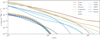 |
Fig. A.1 Spectral plot for non-thermal AQN emission and thermal Bremsstrahlung emission of the hot ICM incorporating the spectra from sample 𝓑. Fornax, being the only galaxy cluster, shows a small region where AQN emission dominates gas emission. |
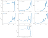 |
Fig. A.2 Radial profiles of |


References
- Abbott, L. F., & Sikivie, P. 1983, Phys. Lett. B, 120, 133 [NASA ADS] [CrossRef] [Google Scholar]
- Abel, C., Afach, S., Ayres, N. J., et al. 2020, Phys. Rev. Lett., 124, 081803 [CrossRef] [PubMed] [Google Scholar]
- Alcock, C., Akerlof, C. W., Allsman, R. A., et al. 1993, Nature, 365, 621 [NASA ADS] [CrossRef] [Google Scholar]
- Alford, M. G., Schmitt, A., Rajagopal, K., & Schäfer, T. 2008, Rev. Mod. Phys., 80, 1455 [NASA ADS] [CrossRef] [Google Scholar]
- Asztalos, S. J., Rosenberg, L. J., van Bibber, K., Sikivie, P., & Zioutas, K. 2006, Ann. Rev. Nucl. Part. Sci., 56, 293 [NASA ADS] [CrossRef] [Google Scholar]
- Aubourg, E., Bareyre, P., Bréhin, S., et al. 1993, Nature, 365, 623 [NASA ADS] [CrossRef] [Google Scholar]
- Bartelmann, M., & Steinmetz, M. 1996, MNRAS, 283, 431 [NASA ADS] [Google Scholar]
- Bennett, C. L., Larson, D., Weiland, J. L., et al. 2013, ApJS, 208, 20 [Google Scholar]
- Blum, K., Sato, R., & Waxman, E. 2017, arXiv e-prints [arXiv:1709.06507] [Google Scholar]
- Böss, L. M. 2023, https://doi.org/10.5281/zenodo.8304965 [Google Scholar]
- Böss, L. M., & Valenzuela, L. M. 2023, https://doi.org/10.5281/zenodo.10145784 [Google Scholar]
- Böss, L. M., Dolag, K., Steinwandel, U. P., et al. 2023, A&A, submitted [arXiv:2310.13734] [Google Scholar]
- Budker, D., Flambaum, V. V., & Zhitnitsky, A. 2022, Symmetry, 14, 459 [NASA ADS] [CrossRef] [Google Scholar]
- Carlsson, K., Karrasch, D., Bauer, N., et al. 2022, https://doi.org/10.5281/zenodo.7468949 [Google Scholar]
- Chang, S., Hagmann, C., & Sikivie, P. 1998, Phys. Rev. D, 59, 023505 [NASA ADS] [CrossRef] [Google Scholar]
- Chapline, G. F. 1975, Nature, 253, 251 [NASA ADS] [CrossRef] [Google Scholar]
- Chen, H., Sun, M., Yagi, M., et al. 2020, MNRAS, 496, 4654 [CrossRef] [Google Scholar]
- Chiang, Y.-K., Overzier, R., & Gebhardt, K. 2013, ApJ, 779, 127 [Google Scholar]
- Crusius, A., & Schlickeiser, R. 1986, A&A, 164, L16 [NASA ADS] [Google Scholar]
- Cuciti, V., Cassano, R., Brunetti, G., et al. 2021, A&A, 647, A51 [EDP Sciences] [Google Scholar]
- Davé, R., Cen, R., Ostriker, J. P., et al. 2001, ApJ, 552, 473 [Google Scholar]
- Dehnen, W., & Aly, H. 2012, MNRAS, 425, 1068 [NASA ADS] [CrossRef] [Google Scholar]
- de Rujula, A., & Glashow, S. L. 1984, Nature, 312, 734 [NASA ADS] [CrossRef] [Google Scholar]
- de Vos, K., Hatch, N. A., Merrifield, M. R., & Mingo, B. 2021, MNRAS, 506, L55 [NASA ADS] [CrossRef] [Google Scholar]
- Di Luzio, L., Giannotti, M., Nardi, E., & Visinelli, L. 2020, Phys. Rept., 870, 1 [NASA ADS] [Google Scholar]
- Dine, M., & Fischler, W. 1983, Phys. Lett. B, 120, 137 [NASA ADS] [CrossRef] [Google Scholar]
- Dine, M., Fischler, W., & Srednicki, M. 1981, Phys. Lett. B, 104, 199 [CrossRef] [Google Scholar]
- Dodelson, S., & Widrow, L. M. 1994, Phys. Rev. Lett., 72, 17 [CrossRef] [Google Scholar]
- Dolag, K., Borgani, S., Schindler, S., Diaferio, A., & Bykov, A. M. 2008, Space Sci. Rev., 134, 229 [Google Scholar]
- Dolag, K., Borgani, S., Murante, G., & Springel, V. 2009, MNRAS, 399, 497 [Google Scholar]
- Dolag, K., Komatsu, E., & Sunyaev, R. 2016, MNRAS, 463, 1797 [Google Scholar]
- Dolag, K., Sorce, J. G., Pilipenko, S., et al. 2023, A&A, 677, A169 [NASA ADS] [CrossRef] [EDP Sciences] [Google Scholar]
- Farhi, E., & Jaffe, R. L. 1984, Phys. Rev. D, 30, 2379 [CrossRef] [Google Scholar]
- Felten, J. E., Gould, R. J., Stein, W. A., & Woolf, N. J. 1969, in Quasars and High-energy Astronomy (Oxford: Oxford University Press), 279 [Google Scholar]
- Flambaum, V. V., & Samsonov, I. B. 2021, Phys. Rev. D, 104, 063042 [NASA ADS] [CrossRef] [Google Scholar]
- Flambaum, V. V., & Samsonov, I. B. 2022a, Phys. Rev. D, 106, 023006 [NASA ADS] [CrossRef] [Google Scholar]
- Flambaum, V. V., & Samsonov, I. B. 2022b, Phys. Rev. D, 105, 123011 [NASA ADS] [CrossRef] [Google Scholar]
- Flambaum, V. V., & Zhitnitsky, A. R. 2019, Phys. Rev., D99, 023517 [Google Scholar]
- Fleury, L., & Moore, G. D. 2016, JCAP, 2016, 004 [CrossRef] [Google Scholar]
- Forbes, M. M., Lawson, K., & Zhitnitsky, A. R. 2010, Phys. Rev. D, 82, 083510 [NASA ADS] [CrossRef] [Google Scholar]
- Fouka, M., & Ouichaoui, S. 2013, Res. Astron. Astrophys., 13, 680 [CrossRef] [Google Scholar]
- Fouka, M., & Ouichaoui, S. 2014, MNRAS, 442, 979 [NASA ADS] [CrossRef] [Google Scholar]
- Ge, S., Liang, X., & Zhitnitsky, A. 2017, Phys. Rev. D, 96, 063514 [NASA ADS] [CrossRef] [Google Scholar]
- Ge, S., Liang, X., & Zhitnitsky, A. 2018, Phys. Rev. D, 97, 043008 [NASA ADS] [CrossRef] [Google Scholar]
- Ge, S., Lawson, K., & Zhitnitsky, A. 2019, Phys. Rev. D, 99, 116017 [NASA ADS] [CrossRef] [Google Scholar]
- Ge, S., Siddiqui, M. S. R., Van Waerbeke, L., & Zhitnitsky, A. 2020, Phys. Rev. D, 102, 123021 [NASA ADS] [CrossRef] [Google Scholar]
- Georgi, H., Kaplan, D. B., & Randall, L. 1986, Phys. Lett. B, 169, 73 [NASA ADS] [CrossRef] [Google Scholar]
- Gorghetto, M., Hardy, E., & Villadoro, G. 2018, J. High Energy Phys., 2018, 151 [CrossRef] [Google Scholar]
- Gorham, P. 2012, Phys. Rev., D86, 123005 [NASA ADS] [Google Scholar]
- Hanisch, R. J. 1982, A&A, 111, 97 [Google Scholar]
- Harikane, Y., Ouchi, M., Ono, Y., et al. 2019, ApJ, 883, 142 [Google Scholar]
- Hawking, S. 1971, MNRAS, 152, 75 [Google Scholar]
- Hernández-Martínez, E., Dolag, K., Seidel, B., et al. 2024, A&A, 687, A253 [NASA ADS] [CrossRef] [EDP Sciences] [Google Scholar]
- Hillas, A. M. 2006, ArXiv e-prints [astro-ph/0607109] [Google Scholar]
- Hu, D., Xu, H., Zhu, Z., et al. 2021, ApJ, 913, 8 [NASA ADS] [CrossRef] [Google Scholar]
- Irastorza, I. G., & Redondo, J. 2018, Prog. Part. Nucl. Phys., 102, 89 [NASA ADS] [CrossRef] [Google Scholar]
- Kawasaki, M., Saikawa, K., & Sekiguchi, T. 2015, Phys. Rev. D, 91, 065014 [NASA ADS] [CrossRef] [Google Scholar]
- Kim, J. E. 1979, Phys. Rev. Lett., 43, 103 [CrossRef] [Google Scholar]
- Klaer, V. B., & Moore, G. D. 2017, JCAP, 2017, 049 [Google Scholar]
- Laureijs, R., Amiaux, J., Arduini, S., et al. 2011, arXiv e-prints [arXiv:1110.3193] [Google Scholar]
- Lawson, K., & Zhitnitsky, A. R. 2008, JCAP, 2008, 022 [CrossRef] [Google Scholar]
- Lawson, K., & Zhitnitsky, A. R. 2019, Phys. Dark Univ., 24, 100295 [NASA ADS] [CrossRef] [Google Scholar]
- Lawson, K., Liang, X., Mead, A., et al. 2019, Phys. Rev. D, 100, 043531 [NASA ADS] [CrossRef] [Google Scholar]
- Liang, X. 2022, PhD thesis, University of British Columbia, Canada [Google Scholar]
- Liang, X., & Zhitnitsky, A. 2016, Phys. Rev. D, 94, 083502 [NASA ADS] [CrossRef] [Google Scholar]
- Liang, X., & Zhitnitsky, A. 2022a, Phys. Rev. D, 106, 063022 [NASA ADS] [CrossRef] [Google Scholar]
- Liang, X., & Zhitnitsky, A. 2022b, Euro. Phys. J. C, 82, 249 [NASA ADS] [CrossRef] [Google Scholar]
- Majidi, F., Liang, X., Waerbeke, L. V., et al. 2024, JCAP, 2024, 045 [CrossRef] [Google Scholar]
- Marsh, D. J. E. 2016, Phys. Rep., 643, 1 [NASA ADS] [CrossRef] [Google Scholar]
- Masso, E. 2003, Nucl. Phys. B Proc. Suppl., 114, 67 [CrossRef] [Google Scholar]
- Masso, E., & Toldra, R. 1995, Phys. Rev. D, 52, 1755 [NASA ADS] [CrossRef] [Google Scholar]
- McNeil Forbes, M., & Zhitnitsky, A. R. 2008a, JCAP, 2008, 023 [CrossRef] [Google Scholar]
- McNeil Forbes, M., & Zhitnitsky, A. R. 2008b, Phys. Rev. D, 78, 083505 [NASA ADS] [CrossRef] [Google Scholar]
- Mori, K., Tomida, H., Nakajima, H., et al. 2022, SPIE Conf. Ser., 12181, 121811T [NASA ADS] [Google Scholar]
- Müller, A., Pfrommer, C., Ignesti, A., et al. 2021, MNRAS, 508, 5326 [CrossRef] [Google Scholar]
- Oaknin, D. H., & Zhitnitsky, A. R. 2005, Phys. Rev. Lett., 94, 101301 [NASA ADS] [CrossRef] [Google Scholar]
- Overzier, R. A. 2016, A&A Rev., 24, 14 [NASA ADS] [CrossRef] [Google Scholar]
- Pal, S., & Kumari, S. 2023, J. Astrophys. Astron., 44, 17 [Google Scholar]
- Palade, D. I., & Pomârjanschi, L. M. 2023, arXiv e-prints [arXiv:2303.13400] [Google Scholar]
- Peccei, R. D., & Quinn, H. R. 1977, Phys. Rev. D, 16, 1791 [CrossRef] [Google Scholar]
- Planck Collaboration XVI. 2014, A&A, 571, A16 [NASA ADS] [CrossRef] [EDP Sciences] [Google Scholar]
- Planck Collaboration Int. X. 2013, A&A, 554, A140 [NASA ADS] [CrossRef] [EDP Sciences] [Google Scholar]
- Preskill, J., Wise, M. B., & Wilczek, F. 1983, Phys. Lett. B, 120, 127 [NASA ADS] [CrossRef] [Google Scholar]
- Raffelt, G. G. 2008, in Lecture Notes in Physics, Axions, eds. M. Kuster, G. Raffelt, & B. Beltrán (Berlin: Springer), 741, 51 [NASA ADS] [CrossRef] [Google Scholar]
- Raza, N., Van Waerbeke, L., & Zhitnitsky, A. 2018, Phys. Rev. D, 98, 103527 [NASA ADS] [CrossRef] [Google Scholar]
- Remus, R.-S., Dolag, K., & Dannerbauer, H. 2023, ApJ, 950, 191 [NASA ADS] [CrossRef] [Google Scholar]
- Rosenberg, L. J. 2015, Proc. Natl. Acad. Sci., 112, 12278 [NASA ADS] [CrossRef] [Google Scholar]
- Rybicki, G. B., & Lightman, A. P. 1986, Radiative Processes in Astrophysics (Hoboken: Wiley) [Google Scholar]
- Santillán, O. P., & Sempé, M. 2020, Euro. Phys. J. C, 80, 466 [CrossRef] [Google Scholar]
- Sarazin, C. L. 1986, Rev. Mod. Phys., 58, 1 [Google Scholar]
- Shi, X., & Fuller, G. M. 1999, Phys. Rev. Lett., 82, 2832 [NASA ADS] [CrossRef] [Google Scholar]
- Shifman, M. A., Vainshtein, A. I., & Zakharov, V. I. 1980, Nucl. Phys. B, 166, 493 [CrossRef] [Google Scholar]
- Sikivie, P. 1982, Phys. Rev. Lett., 48, 1156 [NASA ADS] [CrossRef] [Google Scholar]
- Sikivie, P. 2008, in Lecture Notes in Physics, Axions, eds. M. Kuster, G. Raffelt, & B. Beltrán (Berlin: Springer), 741, 19 [NASA ADS] [CrossRef] [Google Scholar]
- Sikivie, P. 2010, Int. J. Mod. Phys. A, 25, 554 [NASA ADS] [CrossRef] [Google Scholar]
- Sikivie, P. 2021, Rev. Mod. Phys., 93, 015004 [CrossRef] [Google Scholar]
- Sloan, T., VanDevender, J. P., Neilsen, T. B., et al. 2021, Sci. Rep., 11, 22432 [NASA ADS] [CrossRef] [Google Scholar]
- Springel, V., White, S. D. M., Tormen, G., & Kauffmann, G. 2001, MNRAS, 328, 726 [Google Scholar]
- Steigman, G., & Turner, M. S. 1985, Nucl. Phys. B, 253, 375 [NASA ADS] [CrossRef] [Google Scholar]
- Sun, M., Jerius, D., & Jones, C. 2005, ApJ, 633, 165 [NASA ADS] [CrossRef] [Google Scholar]
- Tauber, J. A., Mandolesi, N., Puget, J. L., et al. 2010, A&A, 520, A1 [NASA ADS] [CrossRef] [EDP Sciences] [Google Scholar]
- Terni de Gregory, B., Feretti, L., Giovannini, G., et al. 2017, A&A, 608, A58 [EDP Sciences] [Google Scholar]
- Thierbach, M., Klein, U., & Wielebinski, R. 2003, A&A, 397, 53 [NASA ADS] [CrossRef] [EDP Sciences] [Google Scholar]
- Tully, R. B., Courtois, H. M., Dolphin, A. E., et al. 2013, AJ, 146, 86 [NASA ADS] [CrossRef] [Google Scholar]
- Vallee, J. P. 1988, Ap&SS, 149, 225 [NASA ADS] [CrossRef] [Google Scholar]
- Van Bibber, K., & Rosenberg, L. J. 2006, Phys. Today, 59, 30 [NASA ADS] [CrossRef] [Google Scholar]
- VanDevender, J. P., VanDevender, A. P., Sloan, T., et al. 2017, Sci. Rep., 7, 8758 [NASA ADS] [CrossRef] [Google Scholar]
- VanDevender, J. P., Jerald Buchenauer, C., Cai, C., VanDevender, A. P., & Ulmen, B. A. 2020a, Sci. Rep., 10, 13756 [NASA ADS] [CrossRef] [Google Scholar]
- VanDevender, J. P., Shoemaker, I. M., Sloan, T., VanDevender, A. P., & Ulmen, B. A. 2020b, Sci. Rep., 10, 17903 [NASA ADS] [CrossRef] [Google Scholar]
- VanDevender, J. P., Schmitt, R. G., McGinley, N., et al. 2021a, Universe, 7, 116 [NASA ADS] [CrossRef] [Google Scholar]
- VanDevender, J. P., VanDevender, A. P., Wilson, P., Hammel, B. F., & McGinley, N. 2021b, Universe, 7, 35 [NASA ADS] [CrossRef] [Google Scholar]
- VanDevender, J. P., Sloan, T., & Glissman, M. 2024, Universe, 10, 27 [NASA ADS] [CrossRef] [Google Scholar]
- Van Waerbeke, L., & Zhitnitsky, A. 2019, Phys. Rev. D, 99, 043535 [NASA ADS] [CrossRef] [Google Scholar]
- van Weeren, R. J., de Gasperin, F., Akamatsu, H., et al. 2019, Space Sci. Rev., 215, 16 [Google Scholar]
- Vilenkin, A., & Everett, A. E. 1982, Phys. Rev. Lett., 48, 1867 [NASA ADS] [CrossRef] [Google Scholar]
- Weinberg, S. 1978, Phys. Rev. Lett., 40, 223 [Google Scholar]
- Weniger, E. J., & Cížek, J. 1990, Comp. Phys. Commun., 59, 471 [NASA ADS] [CrossRef] [Google Scholar]
- Wilczek, F. 1978, Phys. Rev. Lett., 40, 279 [Google Scholar]
- Witten, E. 1984, Phys. Rev. D, 30, 272 [CrossRef] [Google Scholar]
- Yang, Z.-H., & Chu, Y.-M. 2017, Journal of Inequalities and Applications, 2017, 41 [CrossRef] [Google Scholar]
- Zel’dovich, Y. B., & Novikov, I. D. 1967, Sov. Astron., 10, 602 [Google Scholar]
- Zhitnitsky, A. R. 1980, Sov. J. Nucl. Phys., 31, 260, [Yad. Fiz.31,497 (1980)] [Google Scholar]
- Zhitnitsky, A. R. 2003, JCAP, 2003, 010 [CrossRef] [Google Scholar]
- Zhitnitsky, A. 2007, Phys. Rev. D, 76, 103518 [NASA ADS] [CrossRef] [Google Scholar]
- Zhitnitsky, A. 2017, JCAP, 2017, 050 [CrossRef] [Google Scholar]
- Zhitnitsky, A. 2018, Phys. Dark Univ., 22, 1 [NASA ADS] [CrossRef] [Google Scholar]
- Zhitnitsky, A. 2021a, Universe, 7, 384 [NASA ADS] [CrossRef] [Google Scholar]
- Zhitnitsky, A. 2021b, J. Phys. G Nucl. Phys., 48, 065201 [NASA ADS] [CrossRef] [Google Scholar]
- Zhitnitsky, A. 2022a, Phys. Lett. B, 828, 137015 [NASA ADS] [CrossRef] [Google Scholar]
- Zhitnitsky, A. 2022b, J. Phys. G Nucl. Phys., 49, 105201 [NASA ADS] [CrossRef] [Google Scholar]
- Zhitnitsky, A. 2023, Phys. Dark Univ., 40, 101217 [NASA ADS] [CrossRef] [Google Scholar]
See original papers on the axion (Peccei & Quinn 1977; Weinberg 1978; Wilczek 1978; Kim 1979; Shifman et al. 1980; Dine et al. 1981; Zhitnitsky 1980) and recent reviews (Van Bibber & Rosenberg 2006; Asztalos et al. 2006; Sikivie 2008; Raffelt 2008; Sikivie 2010; Rosenberg 2015; Marsh 2016; Irastorza & Redondo 2018; Di Luzio et al. 2020; Sikivie 2021).
Here, NDW refers to the number of physically distinct vacua.
In fact, it may resolve a long-standing primordial Lithium puzzle as argued in Flambaum & Zhitnitsky (2019).
All Tables
Cross-identified galaxy clusters with physical properties from the simulation and their ability to show AQN signatures with and without synchrotron radiation in the background at a transition frequency νT in the low-energy regime.
Band-passes for WMAP (Bennett et al. 2013), Planck (Tauber et al. 2010), Euclid (Laureijs et al. 2011) and XRISM (Mori et al. 2022) in units of GHz.
All Figures
|
Fig. 1 Schematic sketch for the antimatter-AQN’s internal structure (not true to scale) with an indication of typical sizes (left panel) and the processes, which lead to the different radiation signatures (middle and right panel). The antimatter-AQN consists of a core of anti-quarks surrounded by positrons. When colliding with the ambient gas, the antimatter-AQN heats up and radiation occurs, which depends on the speed at which the collision occurs, the gas temperature and density as well as the ionization state of the gas. The right panel shows the two key emissions, namely thermal and non-thermal emissions. From an incoming proton (green, small circle), 2 GeV of energy will be available after collision with the AQN. Through annihilation, energetic quarks and gluons are produced and stream either deep within the nugget (around 90% of the 2 GeV) or toward the nugget surface (around 10% of the 2 GeV). Quarks and gluons, which remain inside, will contribute to the thermalization of the nugget. Heat will be transferred from the core to the electrosphere which cools down via thermal Bremsstrahlung emission. Quarks and gluons, which proceed to the surface without thermalization, can transfer energy to positrons and produce non-thermal emission. |
| In the text | |
|
Fig. 2 Spectral range for thermal emission from AQNs. The magnitude and width of a thermal spectrum increase for increasing TAQN and can reach from radio to X-ray frequencies for extraordinary hot AQNs. |
| In the text | |
|
Fig. 3 Non-thermal AQN emission spectrum for different TAQN serving as a validation to reproduce Fig. 3 from Majidi et al. (2024). |
| In the text | |
|
Fig. 4 Histograms of physical properties relevant to the AQN emission. Median values were taken for each mass bin, i.e. for 30 galaxy clusters, respectively. |
| In the text | |
|
Fig. 5 Radial profiles of Δv, Reff, and TAQN mapped onto AQN tracer particles. The median radial profile was taken for each mass bin (i.e. 30 galaxy clusters each) and compared to other mass bins in a region of r ∈ [0,1.5] rvir. |
| In the text | |
|
Fig. 6 Median cluster spectra with lines for each mass bin out of sample 𝒜 over a frequency range of ν ∈ [10−5,108]/(2π)eV. The solid, dash-dot-dotted, dashed, and dash-dotted lines represent AQN thermal emission, non-thermal emission, ICM Bremsstrahlung, and synchrotron emission, respectively. |
| In the text | |
|
Fig. 7 Transition frequency-integrated ratio-relation, color-coded by Mvir with frequency ranges of positive AQN contributions. The low-energy frequency range shows in which the thermal AQN emission dominates. Low cluster masses tend to reside on a tangent, slightly offset towards higher values. The high-energy frequency range shows in which the nonthermal AQN emission dominates. Only AQN emission, originating from the lowest Mvir shows an excess over the thermal gas emission in the high-energy regime. We removed one cluster from the plot where for numerical reasons we could not compute νT and the associated |
| In the text | |
|
Fig. 8 Ratio map expressed in |
| In the text | |
|
Fig. 9 Cross-identified Fornax cluster represented in different relevant properties. |
| In the text | |
|
Fig. 10 Cross-identified Virgo cluster represented in different relevant properties. |
| In the text | |
|
Fig. 11 Fornax cluster AQN, gas, and synchrotron emission generated from WMAP, Planck, Euclid, and XRISM energy ranges. Synchrotron emission is predominantly abundant in WMAP and Planck bands. Thermal gas emission shows the most significant contribution to the background emission in the Euclid and XRISM energy bands. |
| In the text | |
|
Fig. 12 Virgo cluster AQN, gas, and synchrotron emission generated from WMAP, Planck, Euclid, and XRISM energy ranges. Synchrotron emission is predominantly abundant in WMAP and Planck bands. Thermal gas emission shows the most significant contribution to the background emission in Euclid and XRISM energy bands. |
| In the text | |
|
Fig. A.1 Spectral plot for non-thermal AQN emission and thermal Bremsstrahlung emission of the hot ICM incorporating the spectra from sample 𝓑. Fornax, being the only galaxy cluster, shows a small region where AQN emission dominates gas emission. |
| In the text | |
|
Fig. A.2 Radial profiles of |
| In the text | |
Current usage metrics show cumulative count of Article Views (full-text article views including HTML views, PDF and ePub downloads, according to the available data) and Abstracts Views on Vision4Press platform.
Data correspond to usage on the plateform after 2015. The current usage metrics is available 48-96 hours after online publication and is updated daily on week days.
Initial download of the metrics may take a while.