| Issue |
A&A
Volume 691, November 2024
|
|
|---|---|---|
| Article Number | A151 | |
| Number of page(s) | 17 | |
| Section | Astrophysical processes | |
| DOI | https://doi.org/10.1051/0004-6361/202451187 | |
| Published online | 08 November 2024 | |
The complex effect of gas cooling and turbulence on AGN-driven outflow properties
1
Center for Physical Sciences and Technology, Saulėtekio Al. 3, Vilnius LT-10257, Lithuania
2
Institute of Astronomy, University of Cambridge, Madingley Road, Cambridge CB3 0HA, UK
3
Kavli Institute for Cosmology, University of Cambridge, Madingley Road, Cambridge CB3 0HA, UK
⋆ Corresponding author; This email address is being protected from spambots. You need JavaScript enabled to view it.
Received:
19
June
2024
Accepted:
26
August
2024
Abstract
Context. Accretion onto supermassive black holes at close to the Eddington rate is expected to drive powerful winds, which have the potential to majorly influence the properties of the host galaxy. Theoretical models of such winds can simultaneously explain observational correlations between supermassive black holes and their host galaxies, such as the M − σ relation, and the powerful multi-phase outflows that are observed in a number of active galaxies. Analytic models developed to understand these processes usually assume simple galaxy properties, namely spherical symmetry and a smooth gas distribution with an adiabatic equation of state. However, the interstellar medium in real galaxies is clumpy and cooling is important, complicating the analysis.
Aims. We wish to determine how gas turbulence, uneven density distribution, and cooling influence the development of active galactic nucleus (AGN) wind-driven outflows and their global properties on kiloparsec scales.
Methods. We calculated a suite of idealised hydrodynamical simulations of AGN outflows designed to isolate the effects of turbulence and cooling, both separately and in combination. All simulations initially consisted of a 1 kpc gas shell with an AGN in the centre. We measured the main outflow parameters – the velocity, the mass outflow rate (Ṁout), and the momentum (ṗoutc/LAGN) and energy (Ėout/LAGN) loading factors – as the system evolves over 1.2 Myr and estimated plausible observationally derived values.
Results. We find that adiabatic simulations approximately reproduce the analytical estimates of outflow properties independently of the presence or absence of turbulence and clumpiness. Cooling, on the other hand, has a significant effect, reducing the outflow energy rate by one to two orders of magnitude in the smooth simulations and by up to one order of magnitude in the turbulent ones. The interplay between cooling and turbulence depends on AGN luminosity: in Eddington-limited AGN, turbulence enhances the coupling between the AGN wind and the gas, while in lower-luminosity simulations, the opposite is true. This mainly occurs because dense gas clumps are resilient to low-luminosity AGN feedback but get driven away by high-luminosity AGN feedback. The overall properties of multi-phase outflowing gas in our simulations qualitatively agree with observations of multi-phase outflows, although there are some quantitative differences. We also find that using ‘observable’ outflow properties leads to their parameters being underestimated by a factor of a few compared with real values.
Conclusions. We conclude that the AGN wind-driven outflow model is capable of reproducing realistic outflow properties in close-to-realistic galaxy setups and that the M − σ relation can be established without efficient cooling of the shocked AGN wind. Furthermore, we suggest ways to improve large-scale numerical simulations by accounting for the effects of AGN wind.
Key words: black hole physics / ISM: general / ISM: jets and outflows / galaxies: active / galaxies: general / quasars: general
© The Authors 2024
 Open Access article, published by EDP Sciences, under the terms of the Creative Commons Attribution License (https://creativecommons.org/licenses/by/4.0), which permits unrestricted use, distribution, and reproduction in any medium, provided the original work is properly cited.
This article is published in open access under the Subscribe to Open model. This email address is being protected from spambots. You need JavaScript enabled to view it. to support open access publication.
1. Introduction
Observed supermassive black hole (SMBH) scaling relations such as the MBH − σ (Ferrarese & Merritt 2000; Gültekin et al. 2009; McConnell & Ma 2013; Kormendy & Ho 2013; Bennert et al. 2021) and MBH − Mb (Häring & Rix 2004; McConnell & Ma 2013; Kormendy & Ho 2013) relations provide indirect evidence that feedback from active galactic nuclei (AGN) has an impact on the evolution of the host galaxy. More direct observational evidence comes in the form of wide-angle cold gas outflows that extend up to ∼10 kpc from the nucleus (Spence et al. 2016), with mass outflow rates of up to ∼1000 M⊙ yr−1, momentum flow rates of up to ∼50 LAGN/c, and energy flow rates of ∼0.05 − 10% LAGN (Feruglio et al. 2010; Rupke & Veilleux 2011; Sturm et al. 2011; Maiolino et al. 2012; Cicone et al. 2014, 2015; Tombesi et al. 2015; González-Alfonso et al. 2017; Fiore et al. 2017; Fluetsch et al. 2019; Lutz et al. 2020).
In addition to the large-scale outflows, many active galaxies show evidence of fast nuclear winds, with velocities of ∼0.1c (Pounds et al. 2003a,b; Tombesi et al. 2010a,b, 2013), from blueshifted lines observed in the X-ray band, which have subsequently been dubbed ultra-fast outflows (UFOs). Their kinetic power is comparable to that of the large-scale outflows, suggesting a possible physical connection between the two.
There are several theoretical models that attempt to explain the presence of outflows, such as jet-driven cocoons (Gaibler et al. 2012; Bourne & Yang 2023; Talbot et al. 2022, 2024), AGN radiation pressure effects on dusty gas (Ishibashi & Fabian 2015; Thompson et al. 2015; Costa et al. 2018), and AGN wind-driven outflows (Costa et al. 2014; King & Pounds 2015). This last framework provides a connection between UFOs and large-scale outflows by showing that UFOs arise as winds from the AGN accretion disc (King 2010a) that subsequently shock against the interstellar medium (ISM) and reach temperatures of ∼1010 K (e.g. King 2003; Zubovas & King 2012a; Faucher-Giguère & Quataert 2012). The subsequent evolution depends strongly on whether the shocked wind bubble cools efficiently. If it does, then only the wind momentum is transferred to the surrounding gas (e.g. King 2003, 2005; Nayakshin 2014). The condition for the wind to be able to push away most of the surrounding gas is then a SMBH mass MBH ∝ σ4, which is close to the observed relation (King 2010b; Zubovas & King 2012b). Alternatively, if most of the shocked wind energy is available to drive the ISM, a fast, massive, large-scale outflow develops with properties very similar to those observed (Zubovas & King 2012a; Faucher-Giguère & Quataert 2012).
In several galaxies, UFOs and large-scale outflows have been discovered simultaneously (e.g. Feruglio et al. 2015; Tombesi et al. 2015; Veilleux et al. 2017). Although in some cases the energy rates of the two components match almost exactly (e.g. in Mrk 231; see Feruglio et al. 2010, 2015), typically there is a significant discrepancy between the two values (Marasco et al. 2020). There are two primary explanations for this. The first involves AGN luminosity variations over the dynamical timescale of the outflow, tflow ∼ R/vout ∼ 1Rkpcv8−1 Myr, where v8 ≡ vout/1000 km s−1. Since outflow properties cannot change on timescales much shorter than dynamical, it follows that they correlate better with the average AGN luminosity over that time (Zubovas & Nardini 2020). Individual AGN episodes should not last longer than a few times 105 yr (King & Nixon 2015; Schawinski et al. 2015), so the instantaneous luminosity we observe is generally not representative of the long-term average. UFO properties, on the other hand, change on much shorter timescales, of years or less (King & Pounds 2015), and so trace the AGN luminosity much more closely. The inclusion of this variability allows models to reproduce the scatter of large-scale outflow properties when compared against present-day AGN luminosity (Zubovas & Nardini 2020; Zubovas et al. 2022).
The second possible explanation of the variation of outflow properties with regard to UFO and/or AGN properties is uneven coupling in different galaxies. Generally, the ISM exhibits clumping on various scales, with cold dense clouds and filaments embedded in a more diffuse hot component. In this case, most of the shocked wind energy can escape via paths of least resistance (Wagner et al. 2013; Nayakshin 2014; Zubovas & Nayakshin 2014; Bourne et al. 2014; Bieri et al. 2017), namely the low-density channels in the ISM, leaving the cold gas in its wake exposed mostly to the wind momentum. In fact, the fraction of wind energy affecting different clumps runs the gamut from zero to unity (Zubovas & Nayakshin 2014). Many clumps can be compressed by the passage of the outflow, enhancing star formation (Laužikas & Zubovas 2024), facilitating its infall and reducing the effective cross-section of dense clumps exposed to the wind (Bourne et al. 2014). This scenario also helps explain a particular shortcoming of the more idealised, spherically symmetric, wind-driven outflow model. Within that formulation, a momentum-driven outflow can only form if the shocked wind cools efficiently, mainly via the inverse Compton effect (King 2003). The transition between efficient and inefficient cooling should occur on scales of several hundred parsecs; however, the expected signature of radiative cooling on these scales is not observed (Bourne & Nayakshin 2013). In addition, when one considers that the shocked wind plasma is likely two-temperature, with protons carrying most of the energy, it becomes clear that inverse Compton cooling is very inefficient (Faucher-Giguère & Quataert 2012); as such, energy-driven outflows should form very close to the SMBH, clearing gas from the galaxy and preventing the SMBH from growing. The possibility of both momentum- and energy-driven outflows existing and affecting different phases of the gas resolves this issue.
While the behaviour of dense gas in multi-phase outflows has received some attention, the large-scale properties of outflows launched in multi-phase media remain relatively unexplored. In particular, it is uncertain whether the global properties – the kinetic powers, momentum, and mass outflow rates – of the large-scale outflows produced in such systems agree with observational results. Intuitively, we would expect the dense material that comprises the majority of the outflowing mass to move with lower velocities than predicted in the spherically symmetric scenario, with a corresponding decrease in momentum and energy rates and corresponding loading factors. This picture is complicated by the generally non-linear heating and cooling processes, which lead to the outflowing gas changing phase as the outflow evolves (Zubovas & King 2014; Richings & Faucher-Giguère 2018a,b). Although early detections of massive outflows (Feruglio et al. 2010; Sturm et al. 2011; Rupke & Veilleux 2011; Maiolino et al. 2012) generally agreed quite well with the spherically symmetric prediction (Cicone et al. 2014), recent larger outflow samples show much larger scatter around these predictions, primarily towards lower values for a given AGN luminosity (Fluetsch et al. 2019; Lutz et al. 2020).
In this study we used numerical simulations of idealised systems to quantify the distribution and evolution of three major outflow parameters – the mass outflow rate, momentum loading factor, and energy loading factor – in both smooth and turbulent ISM, with and without gas cooling. We show that turbulence by itself does not impact the global parameters (i.e. the energy injected by the AGN couples equally well to smooth and clumpy gas distributions). Cooling, on the other hand, has a profound effect even though we assume that the shocked AGN wind remains adiabatic. The effect of cooling is intertwined with that of gas clumpiness and shock heating by the outflow: in smooth systems, cooling reduces the outflow energy rate by one to two orders of magnitude, with a higher AGN luminosity leading to less efficient cooling; in turbulent systems, the effect is mitigated since some gas can be heated to very high temperatures, leading to inefficient cooling. In general, the mass outflow rates and the momentum and energy loading factors we obtain in simulations with both turbulence and cooling agree quite well with corresponding values of real outflows, and the differences in the host gas density structure go a long way in explaining the observed variety of loading factors.
We briefly review the analytical derivation of outflow parameters in Sect. 2 and present the simulation setup in Sect. 3 and the results in Sect. 4. We discuss the implications of our results in Sect. 5, focusing on their applicability to interpreting outflow observations, the implementation of AGN feedback in numerical simulations, and the shortcomings and possible improvements of our simulations. We summarise the main results and conclude in Sect. 6.
2. Analytical arguments and models
The expansion of energy-driven outflows in a homogeneous medium has been detailed in several papers, including reviews by King & Pounds (2015) and Zubovas & King (2019); here we briefly summarise the main results before considering how we would expect the results to change in an inhomogeneous, clumpy gas distribution. First, it is assumed that the SMBH has reached its formal Mσ mass (King 2005),
 (1)
(1)
where fc = 0.16 is the cosmological baryon fraction, κ = 0.4 cm2 g−1 is the electron scattering opacity and σ200 is the bulge velocity dispersion in units of 200 km s−1. Secondly, feedback is Eddington-limited and the wind has momentum and kinetic energy rates of
 (2)
(2)
and
 (3)
(3)
In the regime in which the wind shock is unable to cool efficiently (i.e. the energy-driven regime), Zubovas & King (2012a) show that most of the wind energy is transferred to the kinetic energy of the outflow such that
 (4)
(4)
and hence
 (5)
(5)
where the AGN wind mass loading ratio
 (6)
(6)
In this equation, fg and fc are the gas fraction and cosmological baryon fraction, respectively, ϵr is the radiative efficiency of accretion, l = LAGN/LEdd and  . For typical galaxy and wind parameters, assuming fg = fc, fL ∼ 400, and so momentum boosts of ∼20 and mass outflow rates of several times 102 − 103 M⊙ yr−1 can be reached.
An important point to note is that the model of Zubovas & King (2012a) assumes that all of the gas is swept up into the outflow. However, let us now assume that the ISM can be split into hot diffuse and cold dense components. We define the parameter
 (7)
(7)
as the fraction of gas in the hot phase. Furthermore, if we assume that only the hot phase can be easily swept up in the energy-driven outflow, with the cold high-density clumps left largely intact (e.g. Bourne et al. 2014), we can define the hot gas mass loading factor as
 (8)
(8)
Replacing fL with fL, hot in the above analysis provides an analytical expectation that when the ISM is clumpy, with large fractions of the gas content contained in dense cold clumps, mass outflow rates and momentum boosts should be considerably tempered when compared with spherically symmetric calculations that assume a homogeneous gas distribution. It is important to note that there is, however, a degeneracy between ηhot and fg and it is also likely that ηhot is a (possibly complicated) function of fg, with gas-rich systems likely being clumpier and hence having smaller values of ηhot. Furthermore, as pointed out in Nayakshin (2014), from the cooling function of Sutherland & Dopita (1993), the hot gas fraction can be given as  , where Z is metallicity in solar units and Rkpc is the radial position within the host galaxy. As a result, more massive, larger, and/or less metal-rich galaxies should have larger hot gas fractions. This also suggests that as outflows move to larger radii, the mass loading and momentum boosts should increase. However, the reality is likely different from the simple picture painted here; this analysis assumes an isothermal gas density distribution, which is only an approximation to the true gas distribution in galaxies. On top of this, the outflow itself will impact ηhot as it propagates, through a combination of ablating and disrupting dense gas clouds and/or compressing gas to high densities as it is swept up. As such, we expect fL to be a complicated function of feedback and galaxy properties.
3. Numerical simulations
While analytical models provide physical intuition, they can take us only so far and as such we now turn to numerical simulations. We adopted a similar setup and methodology to that of simulations previously presented in Bourne et al. (2015), Zubovas et al. (2016), and Zubovas & Maskeliūnas (2023). A modified version of the hydrodynamical code GADGET-3 (Springel 2005), which incorporates the ‘SPHS’ (Read et al. 2010; Read & Hayfield 2012) flavour of SPH (smoothed particle hydrodynamics + switch) and the Wendland kernel (Wendland 1995; Dehnen & Aly 2012), was used for the simulations. The code employs adaptive hydrodynamical smoothing and gravitational softening lengths; the neighbour number is Nngb = 100. The SPH particle mass is mSPH = 940 M⊙.
3.1. Initial conditions
We run two groups of simulations: smooth (labelled ‘Smth’) and turbulent (‘Turb’). In the smooth simulations, the initial conditions consist of a shell of gas between rin = 0.1 kpc and rout = 1 kpc. The density falls with radius as ρ ∝ r−2 and the total mass is Mgas = 9.4 × 10⁸ M⊙, tracked with N = 106 SPH particles. We neglected the self-gravity of the gas to avoid the spurious fragmentation of dense clumps. The shell is embedded in a static singular isothermal sphere background potential with a one-dimensional velocity dispersion of σb = 142 km s−1, corresponding to a background mass Mb = 9.4 × 10⁹ M⊙. Finally, a black hole (BH) particle of mass Mbh = Mσ(σb) = 108 M⊙ is included at the centre of the simulation domain and kept fixed throughout the simulation. All gas particles that fall closer than racc = 0.01 kpc from the BH particle are removed from the simulation.
In the turbulent simulations, the extent of the gas shell is the same, but it is given a turbulent density distribution. To achieve this, we ran a ‘development’ simulation that was identical to the smooth simulations except for the following differences. The gas shell initially extends between rin, d = 0.01 kpc and rout = 1 kpc, has a total mass larger by a factor of ∼1.4 and is given a turbulent velocity field. Turbulence is generated using the method of Dubinski et al. (1995) and Hobbs et al. (2011), which produces a divergence-free turbulent velocity spectrum. The initial characteristic velocity is σt = 149 km s−1 = σb(1+Mgas/Mb)1/2. After 1 Myr, we stopped the simulation and removed the gas in the central rin = 0.1 kpc. The leftover shell now contains N ≃ 106 particles within rout = 1 kpc, which we used as the initial conditions for the turbulent simulations. We repeated this process four times with different random seeds and performed simulations with the four sets of initial conditions. The background potential and BH particle properties in the development and turbulent simulations are identical to those of the smooth simulations.
3.2. Gas thermodynamics
Since we are interested in understanding how outflow properties are affected by a more realistic gas density distribution, we adopted a two-step approach to make the simulation more realistic. The first step is the creation of turbulent initial conditions, as described above. The second step is moving from an adiabatic equation of state, as assumed in the analytical calculations, to one with a realistic radiative cooling prescription, described below. We ran both adiabatic (labelled ‘Adia’) and cooling (labelled ‘Cool’) simulations. In the adiabatic simulations, the initial gas temperature was set to the virial temperature of the background gravitational potential, T ∼ 9.3 × 10⁵ K; we verified that using a lower initial temperature makes no difference to our results.
In the simulations with radiative cooling, we used a combination of two sub-resolution prescriptions. Below temperatures of 104 K, we adopted the function of Mashchenko et al. (2008), which allows gas to cool to 20 K. This cooling function is designed to incorporate the effects of atomic, molecular and dust-mediated cooling in Solar-metallicity gas. This means cooling is particularly efficient; together with the adiabatic simulations, our setup brackets a large range of ‘interesting’ cooling regimes. Above 104 K, we used the prescription of Sazonov et al. (2005), which models the heating and cooling of optically thin gas due to a typical AGN radiation field. We modified this function by neglecting the effect of Compton cooling, a change appropriate for the expected two-temperature plasma nature of the hottest outflowing gas (see Faucher-Giguère & Quataert 2012; Bourne & Nayakshin 2013). The optically thin approximation is unrealistic for the densest clumps, and so our simulations over-predict the heating rate in these regions and hence under-predict the total mass of cold gas. However, in terms of global outflow properties and time-integrated star formation rates, this has a negligible effect (Zubovas & Bourne 2017).
3.3. AGN episode and feedback injection
In all simulations, an AGN is turned on at the start and allowed to continue for the duration of the simulation, until the gas is cleared from the central kiloparsec or falls into the SMBH particle. We ran simulations with different AGN luminosities, labelled ‘L#’, where ‘#’ refers to the luminosity in units of the Eddington luminosity LEdd = 1.26 × 1046 erg/s. Our fiducial simulations are ‘L1’ (i.e. LAGN = LEdd), but we also checked whether the results depend on luminosity by running ‘L0.3’ simulations (i.e. with LAGN = 0.3 LEdd). We also ran four control simulations without an AGN. The AGN affects the gas in two ways: by heating (described in Sect. 3.2 above) and by producing feedback in the form of a fast wind, which we tracked using a novel grid-based scheme. The prescription is described in detail in a companion paper (Tartėnas & Zubovas, in prep.); here we present a summary of the salient points.
The method works by propagating the AGN wind on a static grid, which allows for a quick coupling with co-spatial particles using a spatial hash-like method and a sorted distance matrix. Spatial hashing is used widely outside astronomy (e.g. in collision detection and computer vision; Hastings & Mesit 2005; Teschner et al. 2003; Dong et al. 2021) and was suggested as an effective algorithm for friends-of-friends group finding in astrophysical simulations (Creasey 2018; however, this has been contested by Springel et al. 2021).
We used a modified version of the spherical rectangular equal-area grid (Malkin 2019) and neglected the modification of the θ coordinate. While this modification results in a variation of cell areas of the order of a few per cent, it allows for a simple and quick determination of integer grid indices (r, θ, ϕ) for SPH particles:
 (9)
(9)
 (10)
(10)
 (11)
(11)
where rp, θp, ϕp are SPH particle’s spherical coordinates, Δr, Δθ, Δϕ are the respective grid step sizes, and ⌊x⌋ denotes the floor function.
We used a simple discrete-step approach for wind propagation. First, wind was injected into selected 0-th shell cells, the total energy determined by LAGN and the SMBH timestep. We assumed that AGN wind travels radially outwards at a constant velocity vwind = 0.1c (King 2003, 2010b). Wind propagation was coupled to the SMBH timestep, with timestep limits set by CΔr/vwind, where C = 0.4 is a Courant-type factor.
Feedback is distributed to SPH particles in proportion to those particles’ contribution to the overall density field at the centre of the grid cell. Each wind variable – in our case, energy and momentum – is transferred independently. In the case of momentum injection, if the particle position is outside the cell in question, momentum is injected in the direction of the cell rather than the particle.
3.4. List of simulations
A summary of the main simulation parameters and salient results is given in Table 1. The first column gives the simulation name, and the next three give the main parameters encoded in the name: the type of gas distribution (smooth or turbulent), the presence of radiative cooling (yes or no) and the AGN luminosity. The subsequent columns give the primary results, in the turbulent case averaged over variations in the initial conditions. They are, in order, the outflow velocity, mass outflow rate, momentum loading factor, and energy loading factor. These values are averaged over the extent of the outflow, with the first (second) value in the last three columns using τAGN (τr/v) when averaging (see Eq. (17) and the text below it for the precise definitions used). All values are evaluated at t = 0.5 Myr, when the outflow has already developed but has not yet broken out of the initial shell even in the turbulent simulations. The bottom two rows of the table show analytical predictions for the main results, based on equations in Zubovas & King (2012a), using either the velocity of the contact discontinuity (lower) or the outer shock (higher) for calculations. We note that the analytically estimated values are upper limits, since the velocity calculation depends on the assumption that vout ≫ σb, which allows us to ignore one of the terms in the equation of motion (Zubovas & King 2012a) and the other quantities are calculated using this vout estimate.
Summary of simulations, including key results.
4. Results
We first describe the morphological evolution of gas in all four groups of simulations, as well the evolution of the mass outflow rate (Ṁout), the momentum loading factor ( ), and the energy loading factor (
 ) with radius and with time. We calculated the radial profiles by summing up relevant particle properties over thin shells:
 (12)
(12)
 (13)
(13)
and
 (14)
(14)
where mi and vrad, i are the mass and radial velocity of the ith particle, and the sum is performed over all outflowing particles in the radial bin between r and r + Δr; we use Δr = 0.005 kpc throughout this paper, but the results are insensitive to the precise value as long as Δr ≪ 0.1 kpc. We define a particle to be outflowing if it has vrad > 10 km s−1. The chosen slightly higher threshold value excludes particles that are just nominally outflowing due to stochastic scatter in velocity. We also subtracted the corresponding values calculated in the control (L0) simulation to remove the effect of spurious gas motions; in practice, this is only relevant for the turbulent simulations. The total momentum of the outflow can then be calculated as
 (15)
(15)
and the total energy as
 (16)
(16)
We also defined the global radially and time-averaged values of outflow properties. The mass flow rate is given by
 (17)
(17)
where Mout, corr is the total outflowing mass corrected for spurious motions by subtracting its value in the corresponding control simulation and τout is the age of the outflow. The latter can be defined in two ways. Firstly, from the simulation we directly know the age of the AGN outflow and can simply set τAGN = t, where t is the simulation time. However, this information is not directly available to observers, where it is common to estimate the flow time as τr/v = Rout/vout. The exact values used for Rout and vout can vary between studies and depend upon what assumptions are made about the outflow properties. Such ideas have already been discussed extensively in the literature (see e.g. Rupke et al. 2005; Cicone et al. 2014; Veilleux et al. 2017), including the addition of numerical factors to take the outflow geometry into account (e.g. Maiolino et al. 2012) and the decomposition of the outflow into individual ‘clumps’ (e.g. Cicone et al. 2015; Bischetti et al. 2019). For the simple homogeneous case in which all gas is swept into a shell, Rout and vout could simply be set to the shell radius and velocity. However, here we have two factors to consider: firstly, in the turbulent simulations we do not have a simple, single-velocity thin-shell outflow, and secondly, our ISM shell has an initial inner cavity with rin = 100 pc. Therefore, we set  and
and  , which are the mass-weighted average outflow radius (corrected for the shell inner edge) and radial velocity, respectively. Finally, the averaged momentum and energy rates are then calculated as
  and
and  , respectively, where
  is the mass-weighted average squared radial velocity.
4.1. Gas morphology and outflow rates
4.1.1. Smooth adiabatic simulations
We show the density distribution of a thin (0.1 kpc thickness) slice of the simulation SmthAdiaL1.0 as it evolves in Fig. 1, with the left panel showing a snapshot at t = 0.2 Myr, the middle at 0.5 Myr and the right at 0.8 Myr. As expected, the outflow expands spherically symmetrically, with minor variations only due to finite particle number. The peak density, which corresponds approximately to the contact discontinuity, quickly reaches a velocity vc.d. ≃ 700 km s−1, while the outer edge expands with a velocity vout ≃ 900 km s−1. These values are lower than the analytical estimate by ∼20%. This difference can be explained by several factors. First of all, the analytical estimate, as mentioned, is an upper limit; a more detailed integration of the equation of motion gives a value several per cent lower. Secondly, the simulation does not treat the AGN wind hydrodynamically, so the outflow cavity is filled by a backflow from the shocked gas, further reducing the energy available to push it outwards. The total thermal energy of the gas contained in this hot bubble is ∼50% of the total injected energy; reducing the energy injection by a factor of 2 in the analytical calculation brings the velocity estimate into agreement with the simulated one. Interestingly, the mass-weighted velocity, given in Table 1, is even lower,  km s−1. This happens because the velocity of the density peak is the highest that the gas reaches, while the velocity of the outer edge is the shockwave velocity, which does not correspond to real particle motion. Instead, there are particles getting accelerated towards vc.d. but still have lower velocities, and they bring the average velocity down.
 |
Fig. 1. Gas density integrated through a 0.1 kpc thick slice in simulation SmthAdiaL1.0. The three panels show, from left to right, t = 0.2 Myr, t = 0.5 Myr, and t = 0.8 Myr; brighter colours represent higher gas density. |
Figure 2 shows the radial profiles of the mass outflow rate (top) and the momentum and energy loading factors (middle and bottom, respectively) in the SmthAdiaL1.0 simulation at three times: t = 0.2 Myr (red), t = 0.5 Myr (green), and t = 0.8 Myr (blue). Each radial profile shows a single strong peak with a width increasing with time, from ∼50 pc at t = 0.2 Myr to almost 200 pc at t = 0.8 Myr; again, this is expected and can be intuited from the density map. At all three times, the peak values are significantly higher than the analytical estimates; however, we must keep in mind that they represent values estimated in very narrow radial shells. The globally averaged values, shown by individual circles (for estimates using τAGN) and squares (for estimates using τr/v), essentially agree with the analytical estimates, when accounting for the lower outflow velocity. The trend of values estimated using τr/v being lower than those estimated using the real outflow age is present throughout all simulations, as shown below (Sect. 4.1.5); we discuss the implications of this in Sect. 5.2.
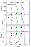 |
Fig. 2. Radial profiles of the mass outflow rate (top), momentum loading factor (middle), and energy loading factor (bottom) in simulations SmthAdiaL1.0 (solid lines and dark points) at t = 0.2 Myr (red), t = 0.5 Myr (green), and t = 0.8 Myr (blue). Lines show the radial profiles calculated using Eqs. (12), (13), and (14), the latter two converted into loading factors. Points show the globally averaged values calculated using τAGN (circles) and τr/v (squares). Grey-shaded areas show the range of analytical estimates. |
Outflow expansion in the SmthAdiaL0.3 simulation is qualitatively identical to that of SmthAdiaL1.0 (Fig. 3). Again, the velocity is lower than the analytical estimate ( km s−1, vc.d. ≃ 400 km s−1), for the same reasons as presented above.
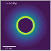 |
Fig. 3. Gas density integrated through a 0.1 kpc thick slice at t = 0.5 Myr in simulation SmthAdiaL0.3. |
4.1.2. Smooth cooling simulations
In Fig. 4 we show the density distribution of the outflow in simulation SmthCoolL1.0 as it evolves. Comparing these plots with Fig. 1, we see that the outflow expands more slowly, with an average velocity ∼300 km s−1, and the expanding region is confined to a narrower, < 50 pc thick, shell. The first difference occurs because the gas in the diffuse outflow cavity cools down and provides less push to the outflowing gas. The second difference occurs because the outflowing gas itself cools down and is compressed into a thinner shell by its own motion. The compressed shell also starts to fragment; this can be seen more clearly when we integrate the density throughout the simulation volume, as shown in Fig. 5. Unlike in similar simulations performed in Nayakshin (2014), the density variations across the shell are not very large: the ratio between top 5% and bottom 5% of density values does not exceed 100. This difference is due to the lack of self-gravity in our setup.
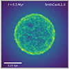 |
Fig. 5. Gas density integrated throughout the simulation volume in simulation SmthCoolL1.0 at t = 0.5 Myr. |
The same behaviour is evident when looking at the radial profiles (Fig. 6). All three integrated parameters have lower values than in the adiabatic simulation. Although the peak values of Ṁ are only slightly lower, the globally integrated values are about twice as small as those in the adiabatic simulation. This happens because, as mentioned above, the outflow shell is much thinner than in the adiabatic simulation. As a result, even though the instantaneous mass flow rate through a given surface is large, the value integrated over the thickness of the shell is lower. The difference is starker for the other parameters and at later times: momentum loading is ∼3.5 times lower at t = 0.5 Myr, while energy loading is ∼8 times lower.
Outflow expansion in simulation SmthCoolL0.3 proceeds along the same lines as in SmthCoolL1.0. The velocity is ∼3 times lower than in SmthCoolL1.0, in contrast to the ∼1.5 ratio between velocities in the two adiabatic simulations. This happens because, at a lower initial velocity, gas in the outflow is heated to lower temperatures where cooling is more efficient. So the fractional loss of energy in this simulation is greater than in the SmthCoolL1.0. The momentum loading factor is actually below unity, so such an outflow, if observed, would be seen as being driven by only the AGN wind momentum.
4.1.3. Turbulent adiabatic simulations
Turning now to the turbulent adiabatic simulations, we show the evolution of the density distribution in Fig. 7. While we can clearly see an expanding outflow, its shape is much more irregular, with different densities along the edge anti-correlated with the outflow distance from the AGN. By t = 0.5 Myr, the outflow reaches the edge of the initial gas distribution at one point; later on, this becomes the site of a champagne outflow extending to very large distances. Radial profiles (Fig. 8) echo the same result: we no longer see a clear sharp peak, but a very widely distributed outflow region. In these plots, the shaded area around each line represents the standard deviation from the mean of the results in four simulations, identical except for a different random seed used to generate the turbulent velocity field (see Sect. 3.1). The position of the maximum mass outflow rate (and, similarly, the maximum momentum and energy loading factors) moves with higher velocity than in the smooth simulations, extending out to almost ∼0.9 kpc by ∼0.8 Myr, giving a radial velocity of ∼1000 km s−1. However, the large amounts of dense gas behind the peak reduce the average velocity to essentially the same as in the smooth simulation. Qualitatively, the same results are visible at other times and in both L1 and L0.3 simulations. Interestingly, the averaged values1 of all parameters are in remarkable agreement between the smooth and turbulent adiabatic simulations. At late times, when parts of the outflow expand beyond Rout, the average velocity begins increasing, while mass and momentum rates start to decrease and the energy rate stays flat (see also Sect. 4.1.5). This, however, is an artefact of the initial conditions.
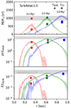 |
Fig. 8. Same as Fig. 2 but for the TurbAdiaL1.0 simulation. Shaded areas show a standard deviation from a sample of four simulations that differ only in terms of the random seed used to generate turbulence. |
Simulation TurbAdiaL0.3 evolves essentially in the same way as TurbAdiaL1.0, except the blowout phase starts around t = 0.8 Myr. The radial profiles are also very similar, and the integrated quantities show basically the same evolution as the higher-luminosity run, with values of the loading factors being very similar to those in the corresponding smooth simulation.
4.1.4. Turbulent cooling simulations
Finally, we arrive at the TurbCoolL1.0 simulation, which has both a turbulent density distribution and gas cooling. Globally, the shape of the outflow (Fig. 9) is similar to that of the TurbAdiaL1.0 simulation, but the cooling outflow has much finer features and higher density contrasts, exceeding four orders of magnitude at distances 0.2 − 0.4 kpc, compared to a ratio of ∼50 outside the outflow. Multiple lobes are visible, separated by dense gas filaments. The average velocity is approximately twice lower than in the TurbAdiaL1.0 simulation but slightly higher than in the SmthCoolL1.0. This happens because the diffuse gas can be pushed away very efficiently, creating a tail of particles with very high radial velocities (v > 1000 km s−1) while a significant fraction of cold gas is still kept from collapsing to the centre very rapidly. The radial distributions of Ṁout and loading factors (Fig. 10) emphasise this: outflowing material is distributed in a very broad shell, ranging from ∼0.25 kpc to > 1 kpc at t = 0.8 Myr, for example. The values of mass flow rate and momentum loading have visible peaks, while the energy loading factor is distributed almost uniformly with radius. The averaged values are a factor of ∼1.5 − 3 lower than analytical estimates.
In simulation TurbCoolL0.3, the features of the TurbCoolL1.0 are even more pronounced. Density ratios are higher, velocity lower, and the radial distribution of the three parameters is almost uniform between the AGN and the outer edge of the outflow. Curiously, this means that the mass flow rate and momentum loading factor in the TurbCoolL0.3 simulation are lower than in the SmthCoolL0.3, reversing the trend seen when comparing other smooth and turbulent analogues.
4.1.5. Time evolution of average outflow properties
In all simulations, outflow properties evolve with time. In the S-ad simulations, the τAGN-evaluations tend to settle to approximately constant values by t = 0.2 Myr (Fig. 11, teal lines); evaluations using τr/v follow the same trend just take longer (0.3 − 0.4 Myr) to reach the plateau. Once the outflow clears the initial gas shell, the mass outflow rate begins to decrease roughly as t−1, because the total outflowing mass remains the same, while τAGN keeps increasing. Due to a corresponding increase in outflow velocity, the momentum loading factor hardly changes and energy loading increases somewhat. This happens because there is less pdV work needed to inflate the gas, so a larger fraction of the input energy is retained as kinetic energy of the outflow. In the cooling simulations (orange lines), all parameters continuously decrease as ever more energy is radiated away.
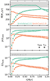 |
Fig. 11. Evolution of the averaged mass outflow rate (top), momentum loading (middle), and energy loading factors (bottom) in the smooth L1.0 simulations with time. Teal and orange lines show estimates of the adiabatic and cooling simulations, respectively. Circles show estimates using τAGN, squares using τr/v. |
In the T-ad simulations (Fig. 12, violet lines), the τAGN-evaluated mass outflow rate reaches a peak at t ∼ 0.3 − 0.5 Myr and begins to decrease as soon as the outflow reaches the edge of the initial shell, eventually settling on the same t−1 trend. The momentum loading factor stays essentially constant, while the energy loading increases as the outflow clears the shell, as in the smooth simulations. The τr/v-evaluated values evolve with a delay, much like their smooth counterparts, and are still growing by t ∼ 0.7 Myr. At this late stage, the velocity increases significantly as ever more of the outflow begins expanding into a vacuum. This leads to the τr/v-estimated values overtaking the τAGN-estimated ones at t ≃ 0.8 Myr and to the energy loading factor increasing significantly.
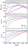 |
Fig. 12. Same as Fig. 11 but for the turbulent simulations. Violet now reflects the adiabatic simulation, while magenta shows the cooling one. |
The T-c simulation evolution (Fig. 12, magenta lines) is remarkably different from the corresponding smooth simulation. Despite energy being radiated away, all parameters keep increasing with time up to ∼0.75 (1) Myr for the τAGN (τr/v) evaluation. At later times, as the outflow escapes the initial shell, mass outflow rates begin to decrease, but momentum loading stays approximately constant, while energy loading keeps increasing. This happens because while outflowing gas has a broad temperature distribution, meaning that cold gas contributes to a significant mass outflow rate, the energy rate (and energy loading factor) is completely dominated by the hot gas, which cools inefficiently. We present this in more detail in Sect. 4.2.
4.1.6. Global effect of turbulence and cooling
For ease of comparison, at a glance, of the effects of cooling, turbulence and both combined on the outflow properties, we plot the average values of the relevant parameters at t = 0.5 Myr in Fig. 13. As in earlier plots, circles show values obtained using τAGN, while squares show those obtained using τr/v. As noted above, there is virtually no difference between the SmthAdiaL1.0 and TurbAdiaL1.0 simulations or between the SmthAdiaL0.3 and TurbAdiaL0.3 ones; that is to say, the addition of turbulence has no detrimental effect on the coupling efficiency of AGN wind momentum and energy to the surrounding ISM. Even though the energy is distributed in a much wider shell in the turbulent simulations, the total energy injection remains the same. In fact, turbulence increases the kinetic energy slightly, because there is more diffuse high-velocity gas in those simulations.
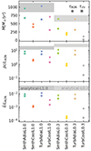 |
Fig. 13. Values of the mass outflow rate (top), momentum loading (middle), and energy loading factors (bottom) in all four L1 simulations at t = 0.7 Myr. The grey area is the analytical prediction. |
When we compare the results of simulations with cooling, a curious pattern emerges: the TurbCoolL1.0 simulation has significantly higher τAGN-evaluated values of all parameters than SmthCoolL1.0. Cooling in the smooth simulation is particularly effective because all of the outflowing material is compressed into a thin and dense shell, while in the turbulent simulations, a lot of the outflowing material remains diffuse and so cools inefficiently. However, in the L0.3 simulations, the trend is reversed for mass and momentum outflow rates: the addition of turbulence leads to a decrease because lower AGN luminosity leads to less hot gas being produced and cooling is overall more efficient.
Overall, the combined effect of turbulence and cooling, when compared with the smooth adiabatic setup, results in a reduction of the mass outflow rate by ∼25% (∼80%), the momentum loading factor by ∼60% (∼93%) and the energy loading factor by ∼63% (∼90%) in the L1 (L0.3) simulations at t = 0.5 Myr. The difference in temporal evolution means that the reduction is greater at earlier times but becomes less significant as the outflow evolves.
4.2. Gas phase distribution
To better understand how the AGN feedback energy couples to the gas and to connect our results to observations of multi-phase outflows, we considered the major outflow properties of cold, warm, and hot gas in the simulations. We mainly present the results for the turbulent simulations with cooling, with a few comments regarding the others when necessary.
In Fig. 14 we show two-dimensional histograms of gas temperature and radial velocity in four turbulent simulations: TurbAdiaL1.0 (top, blue points and lines), TurbCoolL1.0 (bottom) and their corresponding control simulations (grey contours and lines). Gas with temperatures below 104 K exists essentially only in the cooling simulations; we chose a significant drop in particle numbers at T = 3 × 10⁴ K in the TurbCoolL1.0 simulation to delineate cold gas. Gas with temperatures above 107 K exists only in simulations with an AGN; it represents significantly shock-heated gas and we used this temperature to distinguish hot gas. We show these limits with grey horizontal lines in the histograms.
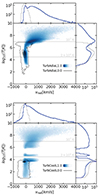 |
Fig. 14. Two-dimensional histograms of gas temperature (vertical axis) against radial velocity (horizontal axis) in the turbulent simulations. Grey contours show corresponding control simulation data. Grey horizontal lines show the criteria for classifying gas as cold, intermediate, or hot. |
We plot the mass outflow rates and the momentum and energy loading factors of gas of the three phases in the TurbCoolL1.0 simulation at t = 0.5 Myr in Fig. 15 and give the averaged values in Table 2. The cold gas dominates the mass outflow rate at distances 0.2 − 0.6 kpc from the nucleus, while hot gas becomes dominant further out. The mass budget is also dominated by cold gas, which comprises ∼70% of the total, followed by hot gas at ∼20%. As expected, hot gas becomes more important when one considers momentum and especially energy loading: the momentum loading factors of hot and cold gas are comparable, while the energy loading factor of the hot gas is several times higher than that of the cold.
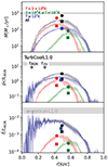 |
Fig. 15. Radial profiles of the mass outflow rate (top), momentum loading (middle), and energy loading factors (bottom) of cold (red lines and points), warm (green), and hot (blue) gas in simulation TurbCoolL1.0 at t = 0.5 Myr. The total values are shown in black. |
Properties of multi-phase gas in the turbulent simulations with cooling.
The radial velocities of gas of different phases show remarkable differences. In the adiabatic simulation, cold gas has a narrow velocity distribution peaking around zero, with maximum velocities vc, max ≃ ±2σb. This represents gas that the outflow has not yet reached. Gas above 106 K shows increased radial velocities, but warm gas has maximum velocities ∼1500 km s−1. Hot gas contains material that has escaped from the initial gas shell and so moves with the highest velocities exceeding even 4000 km s−1. In the TurbCoolL1.0 simulation, there is cold outflowing gas as well, but its velocity does not exceed 1000 km s−1; the same is true for warm gas. Conversely, the hot gas still has very large radial velocities. It is interesting to compare gas velocities with the escape velocity from the simulated galaxy; for a singular isothermal sphere, the escape velocity to infinity is not well defined; instead, we chose resc = 100 kpc as a proxy. Then the escape velocity becomes
 (18)
(18)
where r is the current radial coordinate of the particle. For initial distances 0.1 < r < 1 kpc from the nucleus, the escape velocity range is 4.7σb < vesc < 5.6σb or 667 km s−1 < vesc < 795 km s−1. The fraction of all gas that exceeds this velocity at 0.5 Myr is 3.6%; this number increases to 12% by 0.8 Myr. However, the fraction of escaping cold gas is only 0.19%, increasing to 0.77%. This is consistent with observational results showing that only a small fraction of outflowing material has enough kinetic energy to escape the host galaxy (Fluetsch et al. 2019). On the other hand, more than one-third of hot gas is escaping at 0.5 Myr, increasing to half by 0.8 Myr, reinforcing the point that most of the injected AGN energy is carried away by the hot phase.
The distribution of gas temperatures and velocities in the TurbCoolL0.3 simulation is qualitatively very similar to that in TurbCoolL1.0 (Fig. 16). There is less hot gas, but it still dominates the energy budget. The mean velocities, especially of the cold component, are lower. However, when we look at the velocities required to escape the galaxy, the picture is very different. Only 0.28% of gas is escaping at t = 0.5 Myr, 10 times less than in the higher-luminosity simulation; this number stays essentially the same at 0.8 Myr, suggesting that further energy input is not enough to unbind any more of the gas. When we consider only the cold gas, the escaping fraction is 1.2 × 10⁻⁵, two orders of magnitude lower than in TurbCoolL1.0; by 0.8 Myr, it has increased to 1.1 × 10⁻⁴, still a factor of ∼70 lower than in the higher luminosity run. The fraction of escaping warm gas also increases by almost an order of magnitude, from 0.54% to 4.7%, while the fraction of hot gas increases only a little, from 21% to 27%. This trend of escaping gas fraction with luminosity suggests that there is a threshold, probably around L = LEdd, where even cold gas can be efficiently pushed away by an outflow. Such behaviour agrees with previous simulations (Zubovas & Nayakshin 2014) and represents a way to establish the M − σ relation in the absence of efficient cooling of the shocked AGN wind (Faucher-Giguère & Quataert 2012). We intend to explore the dependence of outflow phases on AGN luminosity and the details of the cooling prescription in a future publication.
5. Discussion
5.1. Comparison with real outflows
In our turbulent simulations with cooling, the cold gas phase dominates the mass budget, comprising 80% (70%) of the mass outflow rate in the L0.3 (L1) simulation. The momentum loading factors of cold gas are comparable to those of the hot, while the energy loading is dominated by the hot component (see Table 2). Furthermore, the hot phase moves with 3−6 times higher velocity and so extends further out – the average radius is ∼15% higher at t = 0.5 Myr (Fig. 15). Looking at the compilations of outflow data from Fiore et al. (2017), Fluetsch et al. (2019), and Lutz et al. (2020), we see that our results qualitatively agree with real outflow parameters. Quantitatively, some discrepancies are present. Real ionised outflows typically have higher velocities,  km s−1, and so do molecular ones,
  km s−1. Both velocities correlate with AGN luminosity; at LAGN ∼ (0.3 − 1)×1046 erg s−1, the mean ionised outflow velocity is the same, while that of molecular outflows increases to ∼650 km s−1. Molecular outflows are observed to have on average higher mass outflow rates at LAGN ∼ 1046 erg s−1 and momentum loading factors, while the energy loading factors are comparable between the two phases. On the other hand, in the few objects where several outflow phases have been detected simultaneously, the molecular phase is dominant both in terms of mass and energy (Fluetsch et al. 2021). Finally, ionised outflows tend to be observed at higher distances of several kpc, while molecular gas is more commonly found in the central kiloparsec, even at LAGN ∼ 1046 erg s−1. So our simulations are underestimating all outflow velocities, but the cold gas velocity is underestimated more; simultaneously, the radial extent of the hot outflow component is underestimated while its mass content is (slightly) overestimated. The reason for the discrepancy in the hot component properties may be the lack of hydrodynamic AGN wind. Because of this, the hot gas phase in our simulations extends inwards towards the AGN, filling the region that, in reality, is taken up by the shocked wind. Furthermore, we did not model the halo gas, which is comparatively very diffuse and would contribute to the hot phase of the outflow. The lack of rapidly moving cold gas may be a consequence of our assumption that the gas is optically thin and the neglect of gas self-gravity. This makes cooling less efficient and precludes the precipitation of cold dense clumps from outflowing hot gas (Nayakshin & Zubovas 2012; Zubovas et al. 2013).
Our simulated outflow properties generally have a rather clear dependence on AGN luminosity. In particular, mean outflow velocities in L1.0 simulations are 1.6−2 times higher than in L0.3, except for the SmthCool simulations, where the ratio is 3.16. The mass outflow rates also differ by a factor of 1.5−2.1, except for TurbCool, where the ratio is an exceptional 6.1. This can be compared with the analytical expectation  , which gives vL1.0/vL0.3 ≃ 1.5. The mass outflow rate ratio in the adiabatic simulations agrees with the expectation, while the velocity ratio is only slightly higher, most likely due to the presence of hot gas filling the outflow cavity, which is fractionally more important in the L0.3 runs. When cooling is introduced, the lower-luminosity AGN heats the gas to lower temperatures, leading to more efficient cooling and a greater difference between the analytical estimate and simulated properties.
Observationally, outflow velocity scales roughly as L0.16 − 0.29 (Fiore et al. 2017); this relationship is flatter than the analytical estimate and much more discrepant with our results. The mass outflow rate, on the other hand, has a steeper dependence on luminosity: Ṁout ∝ L0.76−1.29 (Fiore et al. 2017); this is also discrepant with our results, as it predicts a difference by a factor of 2.5 − 4.7. Understanding why the two relationships differ so much helps explain their difference from the simulated results too. In our analytical estimate,
 (19)
(19)
while the mass outflow rate
 (20)
(20)
In our earlier calculations, we assumed that the only difference between the high- and low-LAGN systems is the AGN luminosity. In reality, the gas velocity dispersion, which is closely related to the galaxy and SMBH masses, has a systematic dependence on LAGN, and the gas fraction may also have such a dependence. Assuming that  , where l ≡ LAGN/LEdd is the Eddington ratio, we find
 (21)
(21)
while the mass outflow rate
 (22)
(22)
We see that even without any correlation between fg and LAGN, we recover almost exactly the observed correlations  and
and  . So the observed correlations can be explained if the different AGN have the same distribution of Eddington ratios, and the luminosity difference arises from the difference in SMBH (and host galaxy) masses, an aspect we did not cover in our simulations. As the number of outflow observations with known SMBH masses increases, it will be interesting to check whether the relationship between outflows in galaxies differing only in AGN Eddington ratio follows our simulated results (and analytical predictions) more closely than the whole population.
5.2. Determining outflow properties from observations
Throughout our simulations, the average outflow properties estimated using τr/v are almost always higher than those estimated using τAGN. In Fig. 17 we plot the ratio of these two timescale estimates as a function of time for all eight non-control simulations. The solid lines correspond to the actual τr/v used when estimating outflow parameters, while dotted lines correspond to the ratio  (i.e. ignoring the presence of the central cavity at the start of the simulation). We see that initially, τr/v can be more than an order of magnitude higher than τAGN (i.e. the real age of the outflow), and generally remains higher throughout the simulations. Only when the outflow breaks out of the initial gas shell, at t > 0.8 Myr in simulations SmthAdiaL1.0, TurbAdiaL1.0 and TurbCoolL1.0, does the ratio drop below unity. This means that using the commonly adopted equation
  provides mass outflow estimates that are up to several times too small. The discrepancy is higher when the AGN luminosity is lower and when the outflow is younger (i.e. closer to the nucleus). This estimate is sometimes multiplied by a factor of a few, which would bring it into an agreement with the real value; however, this multiplication is usually done when trying to account for different outflow geometries (e.g. Cicone et al. 2014; González-Alfonso et al. 2017). We plan to explore the relation between these outflow estimates and geometry in a future paper.
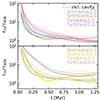 |
Fig. 17. Ratio of the two outflow age estimates, τr/v/τAGN, as a function of time in all simulations. Dotted lines are calculated without accounting for the presence of the initial cavity in the gas distribution. |
5.3. Establishing the M − σ relation
One of the reasons why cooling is much more efficient in the low-luminosity turbulent simulations is the presence of dense gas clumps. While the clumps get slightly heated by the outflow, they cool down quickly and remain resilient to the feedback. They can subsequently fall onto the SMBH and continue feeding and growing it. By t = 0.5 Myr, ∼85% of the cold gas is falling inwards and this number is essentially unchanged by t = 0.8 Myr. In the high-luminosity simulation, the total mass of such clumps is much smaller – ∼45% at t = 0.5 Myr and only ∼13% at t = 0.8 Myr. While we do not have simulations with higher luminosity, we expect this trend to continue: cold gas clumps will be pushed away, heated and dispersed ever more efficiently as the AGN luminosity increases. This confirms a way to establish the M − σ relation without having explicitly momentum-driven outflows (King 2010b), as predicted by considering the two-temperature nature of the shocked wind plasma (Faucher-Giguère & Quataert 2012). At low luminosities, the cold dense clumps, resilient to heating and evaporation, are not pushed by the high-energy outflow and continue feeding the SMBH. As the luminosity increases, the wind momentum becomes high enough to push the dense clumps away, as is happening in the TurbCoolL1.0 simulation. Then the SMBH feeding stops and its mass is established as given by the momentum-driven wind formalism (King 2010b). This has been shown before in idealised simulations with global density gradients (Zubovas & Nayakshin 2014), but here we see the same process working on smaller density inhomogeneities.
5.4. Implementation of AGN feedback in numerical simulations
As noted in Sect. 4.1.1, the lack of hydrodynamic realisation of an AGN wind leads to a reduction in outflow energy by a factor of ∼2. The precise reduction is lower in simulations with turbulence and in simulations with higher luminosity, but these dependences appear weak; there may also be a dependence on gas density. This issue is almost certainly important for cosmological simulations, which typically implement AGN feedback as a simple injection of kinetic and/or thermal energy into the surrounding gas (e.g. Booth & Schaye 2009; Vogelsberger et al. 2014; Tremmel et al. 2017; Davé et al. 2019; Nelson et al. 2019). As the outflow bubble expands in those simulations, the lack of pressure from the presumably extremely hot shocked wind or a thermalising jet leads to a backflow, leaving less energy to push the gas outwards, much like in our simulations.
We envision a few ways to mitigate this issue. The numerically most straightforward way is to double the formal AGN feedback efficiency. However, this would merely mask the problem and would not account for the possible influence of gas density, outflow size and shape. A more realistic solution would be to add a pressure term to the SMBH particle, with the value of this pressure directly proportional to the total injected AGN feedback energy and inversely proportional to the volume of the cavity formed by the shocked wind or jet. The injected energy should be modified by cooling, which becomes important once the AGN luminosity decreases and the wind energy is no longer maintained. The volume of the cavity can be approximated by using the distance to the gas particles neighbouring the SMBH in SPH simulations, and by considering a density threshold in grid-based ones. A drawback of this approach is that the pressure is necessarily isotropic and cannot account for such effects as outflow breakout through low-density channels. A more detailed and anisotropic solution would be to track wind pressure using the same grid that was used for feedback injection (see Sect. 3.3). That way, shocked wind properties can be tracked in each direction independently, providing a continuous push to the gas particles at the inner edge of the outflow cavity.
Of course, the best way of eliminating the problem is to actually treat the wind hydrodynamically. This has been done in AREPO moving-mesh simulations (Costa et al. 2020), where the quasi-relativistic wind is injected into cells neighbouring the SMBH particle, as well as for jet feedback in idealised (Bourne & Sijacki 2017; Talbot et al. 2022, 2024; Ehlert et al. 2023) and cosmological (Bourne et al. 2019; Bourne & Sijacki 2021) simulations, by using novel refinement techniques. In general, improvements of numerical resolution around SMBHs (Curtis & Sijacki 2015; Hopkins et al. 2024) can pave the way to detailed treatments of extreme gas in their vicinity and lead to better prescriptions for making feedback and its effects more realistic (Curtis & Sijacki 2016; Bourne & Sijacki 2017; Koudmani et al. 2019; Talbot et al. 2021).
Another aspect of our results relevant to larger-scale simulations is connected to the spatial resolution. We showed that the uneven density distribution arising due to turbulence interacts with cooling in a non-trivial way. Depending on the AGN luminosity, the clumpiness of gas can either enhance or suppress the mass and momentum rates of the outflow. The connection relies on the gas temperature distribution: diffuse hot gas cools inefficiently, while dense gas can radiate away injected energy very rapidly. In addition to AGN luminosity, the connection almost certainly depends on average gas density and level of turbulence, which determines the typical ratio of densities at a given distance from the nucleus. These results echo the conclusion of Bourne et al. (2015) that low-resolution simulations are better at destroying galaxies via AGN feedback because a more even density distribution does not allow injected energy to escape. Cosmological simulations usually cannot resolve gas with density exceeding nH ∼ 100 cm−3 (e.g. Nelson et al. 2019), corresponding to ρ ∼ 10−22 g cm−3, which is lower than the average gas density on the inside of our simulated shell at the start of the simulations. As the simulation evolves, most of the cold gas, but also some warm and even hot gas attain higher densities (see Fig. 18). As a result, cosmological simulations may overpredict the amount of hot gas in outflows and underpredict the cooling rate of outflowing gas. Even dedicated smaller-scale simulations may be under-predicting the mass of cold dense gas (e.g. Nuza et al. 2014; Valentini et al. 2017). At the same time, cosmological simulations generally do not resolve gas of very low density either, over-predicting the cooling rate. There are two common approaches to mitigating this issue. The first, preventing gas particles that receive AGN feedback injection from cooling for a while (e.g. Tremmel et al. 2017, 2019), does not capture the nuances of this process, leading to an unrealistic distribution of different gas phases. The second method, accumulating AGN feedback energy for a significant period of time (e.g. 25 Myr; see Henden et al. 2018) before injecting it into the gas in one explosive event, misses the gradual development of outflows. Potentially the best way to reduce this problem is to use multi-phase particles (Springel & Hernquist 2003; Murante et al. 2010; Valentini et al. 2017), where each particle (or cell in a grid-based method) is assumed to contain gas of two or three phases, each with distinct temperature and density. Furthermore, improved numerical resolution around shocks and other density discontinuities (Bennett & Sijacki 2020) can help us better track the evolution of multi-phase gas within an outflow.
5.5. Model caveats
In this study we are interested in capturing the effect and interplay of turbulence and cooling of AGN wind-driven outflows. For this reason, our simulations are heavily idealised. While their results can be used to interpret real outflow data and improve large-scale numerical simulations (see the rest of this section), there are many possible improvements.
First of all, in real galaxies, even the central spheroid usually has some angular momentum, which facilitates outflow escape via the polar directions (Zubovas & Nayakshin 2012, 2014; Curtis & Sijacki 2016). This is enhanced further by the presence of a disc. Another effect that may be collimating the large-scale feedback are small-scale anisotropies (i.e. the conical geometry of the AGN wind; Proga & Kallman 2004; Nardini et al. 2015; Luminari et al. 2018). The wind geometry in any particular source is highly uncertain and so would be another free parameter in our simulations. In general, the polar direction of the accretion disc need not line up with the polar direction of the galaxy (as evidenced by the directions of observed AGN jets; Kinney et al. 2000) and the interplay between collimation on different spatial scales can lead to further complexities in outflow geometry.
We neglected gas self-gravity in these simulations, which precludes the formation of very dense clumps and stars. Star formation consumes some material and so reduces the mass outflow rate; simultaneously, stellar feedback may combine with AGN feedback to enhance the energy of outflows.
The cooling function we adopted is also simplified by assuming constant Solar metallicity of the gas. It is well known that more metal-rich gas cools more quickly (Costa et al. 2015) and so will preferentially precipitate out of the outflow. This should lead to the formation of high velocity, high density cold metal-rich gas (Zubovas & King 2014; Richings & Faucher-Giguère 2018a,b). The assumption that gas is optically thin also leads to unrealistically inefficient cooling of dense clumps. These clumps may efficiently transport metal-rich gas to the galactic outskirts, the circumgalactic or even intergalactic medium, affecting the chemical evolution of the galaxy and its environment.
Finally, our assumption of constant AGN luminosity is unrealistic. Both observations (Schawinski et al. 2015) and analytical arguments (King & Nixon 2015) suggest that individual AGN episodes should last only ∼0.1 Myr, although they may be clustered into longer phases of enhanced activity (Hopkins et al. 2007; Zubovas et al. 2022). This finding is corroborated by numerical simulations of realistic accretion of interstellar gas clouds (Alig et al. 2011; Tartėnas & Zubovas 2020, 2022). A ‘flickering’ AGN would interact with gas cooling in a non-linear way, because the cooling timescale of some gas is shorter than the expected downtime between successive AGN episodes, while the hot gas would stay hot throughout.
We plan to address most of these caveats in future works, gradually building up a realistic picture of SMBH accretion and feedback from kiloparsec down to sub-parsec scales. This will both enhance our understanding of real outflows and suggest ways to improve the sub-resolution prescriptions used in large-scale numerical simulations.
6. Summary
In this paper we have presented the results of hydrodynamic simulations of AGN wind-driven outflows in idealised galaxy bulges, focusing on the effects of turbulence, cooling, and their influence on the major properties of the outflows: the mass outflow rate and the momentum and energy loading factors. Our main results are the following:
-
Simulations of smoothly distributed gas under the adiabatic equation of state produce spherically symmetric outflows with properties in general agreement with analytical expectations, except that a significant fraction of the injected energy remains in the outflow cavity where the shocked AGN wind would be in reality; this leads to outflows being slower and having lower momentum and energy than predicted.
-
The addition of turbulence has almost no effect on the coupling between AGN wind and the gas; in fact, the outflows become slightly more energetic in the turbulent simulations.
-
Cooling, on the other hand, has a significant effect, reducing the outflow energy by one to two orders of magnitude in the simulations with smoothly distributed gas and by up to one order of magnitude in the turbulent simulations.
-
The interplay between cooling and turbulence is not straightforward and depends on AGN luminosity: in simulations with LAGN = LEdd, turbulence mitigates cooling by allowing for a large amount of gas to be heated to very high temperatures leading to inefficient cooling, while in simulations with LAGN = 0.3 LEdd, turbulence enhances the effect of cooling on the mass and momentum rates by creating dense gas clumps that are resilient to feedback and can maintain their density by cooling. The destruction of such clumps in the higher luminosity simulations can lead to the establishment of the M − σ relation.
-
In the most realistic simulation – with both turbulence and cooling – cold gas dominates the mass outflow rate, cold and hot gas have similar momentum rates, and the energy rate is dominated by the hot gas. The hot gas has a significantly higher velocity and is distributed farther out than the cold. This agrees qualitatively with the properties of observed outflows.
-
As outflows evolve and break out from the initial gas shell, their velocity increases and the mass outflow rate decreases; the combined effect leads to an increase in the kinetic energy rate.
-
Estimates of average mass outflow rates obtained using the common observational prescription
 almost always underestimate the true values obtained by dividing the total outflowing mass by the age of the outflow. The discrepancy is typically only a factor of < 2 but can be much higher when the outflow is young. Estimates of momentum and energy rates are similarly lower.
These values are the same in simulations with different turbulence seeds, despite the considerable range covered by the shaded areas.
Acknowledgments
We thank Roberto Maiolino and Sergei Nayakshin for their useful comments and discussion on the original draft. MAB acknowledges support from the Science and Technology Facilities Council (STFC). KZ and MT are funded by the Research Council Lithuania grant no. S-MIP-24-100. Some simulations have been performed on Galax, the computing cluster of the Centre for Physical Sciences and Technology in Vilnius, Lithuania.
References
- Alig, C., Burkert, A., Johansson, P. H., & Schartmann, M. 2011, MNRAS, 412, 469 [NASA ADS] [CrossRef] [Google Scholar]
- Bennert, V. N., Treu, T., Ding, X., et al. 2021, ApJ, 921, 36 [NASA ADS] [CrossRef] [Google Scholar]
- Bennett, J. S., & Sijacki, D. 2020, MNRAS, 499, 597 [NASA ADS] [CrossRef] [Google Scholar]
- Bieri, R., Dubois, Y., Rosdahl, J., et al. 2017, MNRAS, 464, 1854 [NASA ADS] [CrossRef] [Google Scholar]
- Bischetti, M., Piconcelli, E., Feruglio, C., et al. 2019, A&A, 628, A118 [NASA ADS] [CrossRef] [EDP Sciences] [Google Scholar]
- Booth, C. M., & Schaye, J. 2009, MNRAS, 398, 53 [Google Scholar]
- Bourne, M. A., & Nayakshin, S. 2013, MNRAS, 436, 2346 [CrossRef] [Google Scholar]
- Bourne, M. A., & Sijacki, D. 2017, MNRAS, 472, 4707 [NASA ADS] [CrossRef] [Google Scholar]
- Bourne, M. A., & Sijacki, D. 2021, MNRAS, 506, 488 [NASA ADS] [CrossRef] [Google Scholar]
- Bourne, M. A., & Yang, H.-Y. K. 2023, Galaxies, 11, 73 [NASA ADS] [CrossRef] [Google Scholar]
- Bourne, M. A., Nayakshin, S., & Hobbs, A. 2014, MNRAS, 441, 3055 [NASA ADS] [CrossRef] [Google Scholar]
- Bourne, M. A., Zubovas, K., & Nayakshin, S. 2015, MNRAS, 453, 1829 [NASA ADS] [CrossRef] [Google Scholar]
- Bourne, M. A., Sijacki, D., & Puchwein, E. 2019, MNRAS, 490, 343 [NASA ADS] [CrossRef] [Google Scholar]
- Cicone, C., Maiolino, R., Sturm, E., et al. 2014, A&A, 562, A21 [NASA ADS] [CrossRef] [EDP Sciences] [Google Scholar]
- Cicone, C., Maiolino, R., Gallerani, S., et al. 2015, A&A, 574, A14 [NASA ADS] [CrossRef] [EDP Sciences] [Google Scholar]
- Costa, T., Sijacki, D., & Haehnelt, M. G. 2014, MNRAS, 444, 2355 [Google Scholar]
- Costa, T., Sijacki, D., & Haehnelt, M. G. 2015, MNRAS, 448, L30 [NASA ADS] [CrossRef] [Google Scholar]
- Costa, T., Rosdahl, J., Sijacki, D., & Haehnelt, M. G. 2018, MNRAS, 479, 2079 [Google Scholar]
- Costa, T., Pakmor, R., & Springel, V. 2020, MNRAS, 497, 5229 [Google Scholar]
- Creasey, P. 2018, Astron. Comput., 25, 159 [NASA ADS] [CrossRef] [Google Scholar]
- Curtis, M., & Sijacki, D. 2015, MNRAS, 454, 3445 [NASA ADS] [CrossRef] [Google Scholar]
- Curtis, M., & Sijacki, D. 2016, MNRAS, 457, L34 [NASA ADS] [CrossRef] [Google Scholar]
- Davé, R., Anglés-Alcázar, D., Narayanan, D., et al. 2019, MNRAS, 486, 2827 [Google Scholar]
- Dehnen, W., & Aly, H. 2012, MNRAS, 425, 1068 [NASA ADS] [CrossRef] [Google Scholar]
- Dong, W., Lao, Y., Kaess, M., & Koltun, V. 2021, ArXiv e-prints [arXiv:2110.00511] [Google Scholar]
- Dubinski, J., Narayan, R., & Phillips, T. G. 1995, ApJ, 448, 226 [NASA ADS] [CrossRef] [Google Scholar]
- Ehlert, K., Weinberger, R., Pfrommer, C., Pakmor, R., & Springel, V. 2023, MNRAS, 518, 4622 [Google Scholar]
- Faucher-Giguère, C.-A., & Quataert, E. 2012, MNRAS, 425, 605 [Google Scholar]
- Ferrarese, L., & Merritt, D. 2000, ApJ, 539, L9 [Google Scholar]
- Feruglio, C., Maiolino, R., Piconcelli, E., et al. 2010, A&A, 518, L155 [NASA ADS] [CrossRef] [EDP Sciences] [Google Scholar]
- Feruglio, C., Fiore, F., Carniani, S., et al. 2015, A&A, 583, A99 [NASA ADS] [CrossRef] [EDP Sciences] [Google Scholar]
- Fiore, F., Feruglio, C., Shankar, F., et al. 2017, A&A, 601, A143 [NASA ADS] [CrossRef] [EDP Sciences] [Google Scholar]
- Fluetsch, A., Maiolino, R., Carniani, S., et al. 2019, MNRAS, 483, 4586 [NASA ADS] [Google Scholar]
- Fluetsch, A., Maiolino, R., Carniani, S., et al. 2021, MNRAS, 505, 5753 [NASA ADS] [CrossRef] [Google Scholar]
- Gaibler, V., Khochfar, S., Krause, M., & Silk, J. 2012, MNRAS, 425, 438 [NASA ADS] [CrossRef] [Google Scholar]
- González-Alfonso, E., Fischer, J., Spoon, H. W. W., et al. 2017, ApJ, 836, 11 [Google Scholar]
- Gültekin, K., Richstone, D. O., Gebhardt, K., et al. 2009, ApJ, 698, 198 [Google Scholar]
- Häring, N., & Rix, H.-W. 2004, ApJ, 604, L89 [Google Scholar]
- Hastings, E., & Mesit, J. 2005, Optimization of Large-scale, Real-time Simulations by Spatial Hashing, https://stars.library.ucf.edu/scopus2000/3140 [Google Scholar]
- Henden, N. A., Puchwein, E., Shen, S., & Sijacki, D. 2018, MNRAS, 479, 5385 [CrossRef] [Google Scholar]
- Hobbs, A., Nayakshin, S., Power, C., & King, A. 2011, MNRAS, 413, 2633 [NASA ADS] [CrossRef] [Google Scholar]
- Hopkins, P. F., Hernquist, L., Cox, T. J., Robertson, B., & Krause, E. 2007, ApJ, 669, 67 [NASA ADS] [CrossRef] [Google Scholar]
- Hopkins, P. F., Grudic, M. Y., Su, K.-Y., et al. 2024, Open J. Astrophys., 7, 18 [NASA ADS] [Google Scholar]
- Ishibashi, W., & Fabian, A. C. 2015, MNRAS, 451, 93 [NASA ADS] [CrossRef] [Google Scholar]
- King, A. 2003, ApJ, 596, L27 [Google Scholar]
- King, A. 2005, ApJ, 635, L121 [Google Scholar]
- King, A. R. 2010a, MNRAS, 408, L95 [Google Scholar]
- King, A. R. 2010b, MNRAS, 402, 1516 [Google Scholar]
- King, A., & Nixon, C. 2015, MNRAS, 453, L46 [NASA ADS] [CrossRef] [Google Scholar]
- King, A., & Pounds, K. 2015, ARA&A, 53, 115 [NASA ADS] [CrossRef] [Google Scholar]
- Kinney, A. L., Schmitt, H. R., Clarke, C. J., et al. 2000, ApJ, 537, 152 [Google Scholar]
- Kormendy, J., & Ho, L. C. 2013, ARA&A, 51, 511 [Google Scholar]
- Koudmani, S., Sijacki, D., Bourne, M. A., & Smith, M. C. 2019, MNRAS, 484, 2047 [NASA ADS] [CrossRef] [Google Scholar]
- Laužikas, M., & Zubovas, K. 2024, A&A, 690, A396 [NASA ADS] [CrossRef] [EDP Sciences] [Google Scholar]
- Luminari, A., Piconcelli, E., Tombesi, F., et al. 2018, A&A, 619, A149 [NASA ADS] [CrossRef] [EDP Sciences] [Google Scholar]
- Lutz, D., Sturm, E., Janssen, A., et al. 2020, A&A, 633, A134 [NASA ADS] [CrossRef] [EDP Sciences] [Google Scholar]
- Maiolino, R., Gallerani, S., Neri, R., et al. 2012, MNRAS, 425, L66 [Google Scholar]
- Malkin, Z. 2019, AJ, 158, 158 [NASA ADS] [CrossRef] [Google Scholar]
- Marasco, A., Cresci, G., Nardini, E., et al. 2020, A&A, 644, A15 [EDP Sciences] [Google Scholar]
- Mashchenko, S., Wadsley, J., & Couchman, H. M. P. 2008, Science, 319, 174 [NASA ADS] [CrossRef] [Google Scholar]
- McConnell, N. J., & Ma, C.-P. 2013, ApJ, 764, 184 [Google Scholar]
- Murante, G., Monaco, P., Giovalli, M., Borgani, S., & Diaferio, A. 2010, MNRAS, 405, 1491 [NASA ADS] [Google Scholar]
- Nardini, E., Reeves, J. N., Gofford, J., et al. 2015, Science, 347, 860 [Google Scholar]
- Nayakshin, S. 2014, MNRAS, 437, 2404 [Google Scholar]
- Nayakshin, S., & Zubovas, K. 2012, MNRAS, 427, 372 [Google Scholar]
- Nelson, D., Pillepich, A., Springel, V., et al. 2019, MNRAS, 490, 3234 [Google Scholar]
- Nuza, S. E., Parisi, F., Scannapieco, C., et al. 2014, MNRAS, 441, 2593 [NASA ADS] [CrossRef] [Google Scholar]
- Pounds, K. A., Reeves, J. N., King, A. R., et al. 2003a, MNRAS, 345, 705 [Google Scholar]
- Pounds, K. A., King, A. R., Page, K. L., & O’Brien, P. T. 2003b, MNRAS, 346, 1025 [Google Scholar]
- Proga, D., & Kallman, T. R. 2004, ApJ, 616, 688 [Google Scholar]
- Read, J. I., & Hayfield, T. 2012, MNRAS, 422, 3037 [NASA ADS] [CrossRef] [Google Scholar]
- Read, J. I., Hayfield, T., & Agertz, O. 2010, MNRAS, 405, 1513 [NASA ADS] [Google Scholar]
- Richings, A. J., & Faucher-Giguère, C.-A. 2018a, MNRAS, 474, 3673 [Google Scholar]
- Richings, A. J., & Faucher-Giguère, C.-A. 2018b, MNRAS, 478, 3100 [NASA ADS] [CrossRef] [Google Scholar]
- Rupke, D. S. N., & Veilleux, S. 2011, ApJ, 729, L27 [NASA ADS] [CrossRef] [Google Scholar]
- Rupke, D. S., Veilleux, S., & Sanders, D. B. 2005, ApJS, 160, 115 [Google Scholar]
- Sazonov, S. Y., Ostriker, J. P., Ciotti, L., & Sunyaev, R. A. 2005, MNRAS, 358, 168 [NASA ADS] [CrossRef] [Google Scholar]
- Schawinski, K., Koss, M., Berney, S., & Sartori, L. F. 2015, MNRAS, 451, 2517 [Google Scholar]
- Spence, R. A. W., Zaurín, J. R., Tadhunter, C. N., et al. 2016, MNRAS, 459, L16 [NASA ADS] [CrossRef] [Google Scholar]
- Springel, V. 2005, MNRAS, 364, 1105 [Google Scholar]
- Springel, V., & Hernquist, L. 2003, MNRAS, 339, 289 [Google Scholar]
- Springel, V., Pakmor, R., Zier, O., & Reinecke, M. 2021, MNRAS, 506, 2871 [NASA ADS] [CrossRef] [Google Scholar]
- Sturm, E., González-Alfonso, E., Veilleux, S., et al. 2011, ApJ, 733, L16 [NASA ADS] [CrossRef] [Google Scholar]
- Sutherland, R. S., & Dopita, M. A. 1993, ApJS, 88, 253 [Google Scholar]
- Talbot, R. Y., Bourne, M. A., & Sijacki, D. 2021, MNRAS, 504, 3619 [NASA ADS] [CrossRef] [Google Scholar]
- Talbot, R. Y., Sijacki, D., & Bourne, M. A. 2022, MNRAS, 514, 4535 [NASA ADS] [CrossRef] [Google Scholar]
- Talbot, R. Y., Sijacki, D., & Bourne, M. A. 2024, MNRAS, 528, 5432 [NASA ADS] [CrossRef] [Google Scholar]
- Tartėnas, M., & Zubovas, K. 2020, MNRAS, 492, 603 [CrossRef] [Google Scholar]
- Tartėnas, M., & Zubovas, K. 2022, MNRAS, 516, 2522 [CrossRef] [Google Scholar]
- Teschner, M., Heidelberger, B., Müller, M., Pomerantes, D., & Gross, M. H. 2003, International Symposium on Vision, Modeling, and Visualization, https://api.semanticscholar.org/CorpusID:12035329 [Google Scholar]
- Thompson, T. A., Fabian, A. C., Quataert, E., & Murray, N. 2015, MNRAS, 449, 147 [NASA ADS] [CrossRef] [Google Scholar]
- Tombesi, F., Cappi, M., Reeves, J. N., et al. 2010a, A&A, 521, A57 [NASA ADS] [CrossRef] [EDP Sciences] [Google Scholar]
- Tombesi, F., Sambruna, R. M., Reeves, J. N., et al. 2010b, ApJ, 719, 700 [NASA ADS] [CrossRef] [Google Scholar]
- Tombesi, F., Cappi, M., Reeves, J. N., et al. 2013, MNRAS, 430, 1102 [Google Scholar]
- Tombesi, F., Meléndez, M., Veilleux, S., et al. 2015, Nature, 519, 436 [NASA ADS] [CrossRef] [Google Scholar]
- Tremmel, M., Karcher, M., Governato, F., et al. 2017, MNRAS, 470, 1121 [NASA ADS] [CrossRef] [Google Scholar]
- Tremmel, M., Quinn, T. R., Ricarte, A., et al. 2019, MNRAS, 483, 3336 [CrossRef] [Google Scholar]
- Valentini, M., Murante, G., Borgani, S., et al. 2017, MNRAS, 470, 3167 [CrossRef] [Google Scholar]
- Veilleux, S., Bolatto, A., Tombesi, F., et al. 2017, ApJ, 843, 18 [Google Scholar]
- Vogelsberger, M., Genel, S., Springel, V., et al. 2014, MNRAS, 444, 1518 [Google Scholar]
- Wagner, A. Y., Umemura, M., & Bicknell, G. V. 2013, ApJ, 763, L18 [NASA ADS] [CrossRef] [Google Scholar]
- Wendland, H. 1995, Adv. Comput. Math., 4, 389 [CrossRef] [MathSciNet] [Google Scholar]
- Zubovas, K., & Bourne, M. A. 2017, MNRAS, 468, 4956 [NASA ADS] [CrossRef] [Google Scholar]
- Zubovas, K., & King, A. 2012a, ApJ, 745, L34 [Google Scholar]
- Zubovas, K., & King, A. R. 2012b, MNRAS, 426, 2751 [NASA ADS] [CrossRef] [Google Scholar]
- Zubovas, K., & King, A. R. 2014, MNRAS, 439, 400 [Google Scholar]
- Zubovas, K., & King, A. R. 2019, Gen. Relat. Grav., 51, 65 [CrossRef] [Google Scholar]
- Zubovas, K., & Maskeliūnas, G. 2023, MNRAS, 524, 4819 [CrossRef] [Google Scholar]
- Zubovas, K., & Nardini, E. 2020, MNRAS, 498, 3633 [Google Scholar]
- Zubovas, K., & Nayakshin, S. 2012, MNRAS, 424, 666 [NASA ADS] [CrossRef] [Google Scholar]
- Zubovas, K., & Nayakshin, S. 2014, MNRAS, 440, 2625 [NASA ADS] [CrossRef] [Google Scholar]
- Zubovas, K., Nayakshin, S., Sazonov, S., & Sunyaev, R. 2013, MNRAS, 431, 793 [NASA ADS] [CrossRef] [Google Scholar]
- Zubovas, K., Bourne, M. A., & Nayakshin, S. 2016, MNRAS, 457, 496 [NASA ADS] [CrossRef] [Google Scholar]
- Zubovas, K., Bialopetravičius, J., & Kazlauskaitė, M. 2022, MNRAS, 515, 1705 [CrossRef] [Google Scholar]
All Tables
All Figures
|
Fig. 1. Gas density integrated through a 0.1 kpc thick slice in simulation SmthAdiaL1.0. The three panels show, from left to right, t = 0.2 Myr, t = 0.5 Myr, and t = 0.8 Myr; brighter colours represent higher gas density. |
| In the text | |
|
Fig. 2. Radial profiles of the mass outflow rate (top), momentum loading factor (middle), and energy loading factor (bottom) in simulations SmthAdiaL1.0 (solid lines and dark points) at t = 0.2 Myr (red), t = 0.5 Myr (green), and t = 0.8 Myr (blue). Lines show the radial profiles calculated using Eqs. (12), (13), and (14), the latter two converted into loading factors. Points show the globally averaged values calculated using τAGN (circles) and τr/v (squares). Grey-shaded areas show the range of analytical estimates. |
| In the text | |
|
Fig. 3. Gas density integrated through a 0.1 kpc thick slice at t = 0.5 Myr in simulation SmthAdiaL0.3. |
| In the text | |
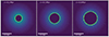 |
Fig. 4. Same as Fig. 1 but for the SmthCoolL1.0 simulation. |
| In the text | |
|
Fig. 5. Gas density integrated throughout the simulation volume in simulation SmthCoolL1.0 at t = 0.5 Myr. |
| In the text | |
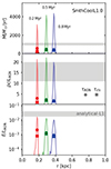 |
Fig. 6. Same as Fig. 2 but for the SmthCoolL1.0 simulation. |
| In the text | |
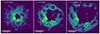 |
Fig. 7. Same as Fig. 1 but for the TurbAdiaL1.0 simulation. |
| In the text | |
|
Fig. 8. Same as Fig. 2 but for the TurbAdiaL1.0 simulation. Shaded areas show a standard deviation from a sample of four simulations that differ only in terms of the random seed used to generate turbulence. |
| In the text | |
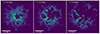 |
Fig. 9. Same as Fig. 1 but for the TurbCoolL1.0 simulation. |
| In the text | |
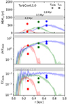 |
Fig. 10. Same as Fig. 8 but for the TurbCoolL1.0 simulation. |
| In the text | |
|
Fig. 11. Evolution of the averaged mass outflow rate (top), momentum loading (middle), and energy loading factors (bottom) in the smooth L1.0 simulations with time. Teal and orange lines show estimates of the adiabatic and cooling simulations, respectively. Circles show estimates using τAGN, squares using τr/v. |
| In the text | |
|
Fig. 12. Same as Fig. 11 but for the turbulent simulations. Violet now reflects the adiabatic simulation, while magenta shows the cooling one. |
| In the text | |
|
Fig. 13. Values of the mass outflow rate (top), momentum loading (middle), and energy loading factors (bottom) in all four L1 simulations at t = 0.7 Myr. The grey area is the analytical prediction. |
| In the text | |
|
Fig. 14. Two-dimensional histograms of gas temperature (vertical axis) against radial velocity (horizontal axis) in the turbulent simulations. Grey contours show corresponding control simulation data. Grey horizontal lines show the criteria for classifying gas as cold, intermediate, or hot. |
| In the text | |
|
Fig. 15. Radial profiles of the mass outflow rate (top), momentum loading (middle), and energy loading factors (bottom) of cold (red lines and points), warm (green), and hot (blue) gas in simulation TurbCoolL1.0 at t = 0.5 Myr. The total values are shown in black. |
| In the text | |
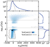 |
Fig. 16. Same as Fig. 14 but for the TurbCoolL0.3 simulation. |
| In the text | |
|
Fig. 17. Ratio of the two outflow age estimates, τr/v/τAGN, as a function of time in all simulations. Dotted lines are calculated without accounting for the presence of the initial cavity in the gas distribution. |
| In the text | |
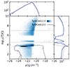 |
Fig. 18. Same as Fig. 14 but showing the relationship between gas temperature and density. |
| In the text | |
Current usage metrics show cumulative count of Article Views (full-text article views including HTML views, PDF and ePub downloads, according to the available data) and Abstracts Views on Vision4Press platform.
Data correspond to usage on the plateform after 2015. The current usage metrics is available 48-96 hours after online publication and is updated daily on week days.
Initial download of the metrics may take a while.