Dynamical resonances in PHANGS galaxies

Marina Ruiz-García; Miguel Querejeta; Santiago García-Burillo; Eric Emsellem; Sharon E. Meidt; Mattia C. Sormani; Eva Schinnerer; Thomas G. Williams; Zein Bazzi; Dario Colombo; Damian R. Gleis; Oleg Y. Gnedin; Ralf S. Klessen; Adam K. Leroy; Patricia Sánchez-Blázquez; Sophia K. Stuber

doi:10.1051/0004-6361/202450935

Home

All issues

Volume 691 (November 2024)

A&A, 691 (2024) A351

Full HTML

Open Access

Issue		A&A Volume 691, November 2024


Article Number		A351
Number of page(s)		21
Section		Extragalactic astronomy
DOI		https://doi.org/10.1051/0004-6361/202450935
Published online		27 November 2024

A&A, 691, A351 (2024)

Dynamical resonances in PHANGS galaxies

Marina Ruiz-García¹^⋆, Miguel Querejeta¹, Santiago García-Burillo¹, Eric Emsellem²^,3, Sharon E. Meidt⁴, Mattia C. Sormani⁵, Eva Schinnerer⁶, Thomas G. Williams⁷, Zein Bazzi⁸, Dario Colombo⁸, Damian R. Gleis⁶, Oleg Y. Gnedin⁹, Ralf S. Klessen¹⁰, Adam K. Leroy¹¹, Patricia Sánchez-Blázquez¹² and Sophia K. Stuber⁶

¹ Observatorio Astronómico Nacional (IGN), C/Alfonso XII, 3, E-28014 Madrid, Spain
² European Southern Observatory, Karl-Schwarzschild Straße 2, D-85748 Garching bei München, Germany
³ Univ. Lyon, Univ. Lyon 1, ENS de Lyon, CNRS, Centre de Recherche Astrophysique de Lyon UMR5574, F-69230 Saint-Genis-Laval, France
⁴ Sterrenkundig Observatorium, Universiteit Gent, Krijgslaan 281 S9, B-9000 Gent, Belgium
⁵ Università dell’Insubria, via Valleggio 11, 22100 Como, Italy
⁶ Max-Planck-Institut für Astronomie, Königstuhl 17, D-69117 Heidelberg, Germany
⁷ Sub-department of Astrophysics, Department of Physics, University of Oxford, Keble Road, Oxford OX1 3RH, UK
⁸ Argelander-Institut für Astronomie, Universität Bonn, Auf dem Hügel 71, 53121 Bonn, Germany
⁹ Department of Astronomy, University of Michigan, Ann Arbor, MI 48109, USA
¹⁰ Universität Heidelberg, Zentrum für Astronomie, Albert-Ueberle-Str. 2, 69120 Heidelberg, Germany
¹¹ Department of Astronomy, The Ohio State University, 140 West 18th Avenue, Columbus, Ohio 43210, USA
¹² Departamento de Física de la Tierra y Astrofísica, Universidad Complutense de Madrid, E-28040, Madrid, Spain

^⋆ Corresponding author; m.ruiz@oan.es

Received: 31 May 2024
Accepted: 4 October 2024

Abstract

Bars are remarkable stellar structures that can transport gas toward centers and drive the secular evolution of galaxies. In this context, it is important to locate dynamical resonances associated with bars. For this study, we used Spitzer near-infrared images as a proxy for the stellar gravitational potential and the ALMA CO(J = 2–1) gas distribution from the PHANGS survey to determine the position of the main dynamical resonances associated with the bars in the PHANGS sample of 74 nearby star-forming galaxies. We used the gravitational torque method to estimate the location of the bar corotation radius (R_CR), where stars and gas rotate at the same angular velocity as the bar. Of the 46 barred galaxies in PHANGS, we have successfully determined the corotation (CR) for 38 of them. The mean ratio of the R_CR to the bar radius (R_bar) is ℛ = R_CR/R_bar = 1.12, with a standard deviation of 0.39. This is consistent with the average value expected from theory and suggests that bars are predominantly fast. We also compared our results with other bar CR measurements from the literature, which employ different methods, and find good agreement (ρ = 0.64). Finally, using rotation curves, we have estimated other relevant resonances such as the inner Lindblad resonance (ILR) and the outer Lindblad resonance (OLR), which are often associated with rings. This work provides a useful catalog of resonances for a large sample of nearby galaxies and emphasizes the clear connection between bar dynamics and morphology.

Key words: galaxies: kinematics and dynamics / galaxies: photometry / galaxies: structure

© The Authors 2024

Open Access article, published by EDP Sciences, under the terms of the Creative Commons Attribution License (https://creativecommons.org/licenses/by/4.0), which permits unrestricted use, distribution, and reproduction in any medium, provided the original work is properly cited.

This article is published in open access under the Subscribe to Open model. Subscribe to A&A to support open access publication.

1. Introduction

A longstanding challenge in modern astrophysics is understanding and characterizing how galactic structures can drive galaxy evolution through the redistribution of gas. It is widely known that gas is drawn inward by asymmetries in the gravitational potential, such as those induced by bars (Roberts et al. 1979; Simkin et al. 1980; van Albada & Roberts 1981; Hasan & Norman 1990; Pfenniger & Norman 1990; Friedli & Benz 1993; Sakamoto et al. 1999; Mundell & Shone 1999; Athanassoula 2000; Jogee 2006; Haan et al. 2009). Other non-axisymmetries in the gravitational potential can also result in gas inflow including the following: nuclear warps (Schinnerer et al. 2000), nuclear spirals (Combes et al. 2014), secondary bars within large scale bars (Shlosman et al. 1989; Friedli & Martinet 1993; Maciejewski & Sparke 2000; Heller et al. 2001; Shlosman & Heller 2002; Englmaier & Shlosman 2004), and m = 1 perturbations (Shu et al. 1990; Junqueira & Combes 1996; García-Burillo et al. 2000). Other nongravitational mechanisms have also been advocated for to explain the radial redistribution of the gas, such as viscous torques and dynamical friction between large molecular clouds and stars (Shakura & Sunyaev 1973; Pringle 1981; Balbus & Hawley 1998; Combes 2002, 2004; García-Burillo et al. 2005).

Dynamical resonances, such as the corotation (CR) or the Lindblad resonances, represent important locations in spiral galaxies, where the angular frequency Ω of a particle rotating with the disk, such as a star, is related to the angular frequency of the rotating pattern (e.g., bar or spiral pattern) Ω_p, as follows:

$\begin{matrix} Ω = Ω_{p} + \frac{l}{m} κ, \end{matrix}$ $\begin{aligned} \Omega = \Omega _{\rm p} + \frac{l}{m}\kappa , \end{aligned}$ (1)

where κ is the epicyclic frequency, and m and l are integer numbers¹ (Binney & Tremaine 1987). At the CR, the stars and the rotating density pattern rotate at the same angular velocity, Ω_p, known as the pattern speed, that is, Ω(CR) = Ω_p. In this work we specifically focus on the bar.

The ratio between the corotation radius R_CR and the bar length R_bar is referred to as ℛ, and is typically used to differentiate between fast and slow bars. As the pattern speed Ω = v/R typically decreases with radius, for a fixed R_bar, the distance-independent ratio ℛ increases if the bar rotates slower (a lower Ω_bar, implying that CR is further out). Debattista & Sellwood (2000) proposed a classification where fast bars are the ones that appear in galaxies with 1 < ℛ < 1.4, while slow bars are the ones with ℛ > 1.4. Later, Buta & Zhang (2009) and Aguerri et al. (2015) added “ultra-fast bars” (ℛ < 1) to this classification. This is the nomenclature we subsequently follow in the paper. We note that ultra-fast bars are, in most cases, compatible with fast bars within error bars in the literature (see references in Table D.1).

The existence of fast and slow bars has cosmological implications for the braking of bars over time (Debattista & Sellwood 2000), as the dynamical friction with dark matter can produce a “slowdown” of the bars, increasing the R_CR (Tremaine & Weinberg 1984b; Chiba 2023). Even though one could think the amount of dark matter in the inner parts of galaxies can be inferred from ℛ, this determination is far from straightforward (see Athanassoula 2014). According to the simulation work of Athanassoula (1992), the range ℛ ∼ 1.2 ± 0.2 is favored. This is also supported by other simulations (e.g., Debattista & Sellwood 2000) and by observational results that show that most bars have 1 < ℛ < 1.4 (e.g., Corsini 2011; Guo et al. 2019; Cuomo et al. 2021 or Garma-Oehmichen et al. 2022; all of them studied a sample focused on late-type barred galaxies, using the Tremaine-Weinberg method, Tremaine & Weinberg 1984a, and relied on rotation curves to infer R_CR from Ω_p). It is important to note, however, that recent studies such as Font et al. (2017) do not agree on the interpretation that 1 < ℛ < 1.4 implies that bars necessarily rotate faster than bars with a larger ℛ, as explained in Sect. 5.

The R_CR (and other resonances) have been estimated through many different methods. The most common ones include (1) the Tremaine-Weinberg method (hereafter TW method or TW), which is a kinematic method that considers measurements of the velocity field along a set of long slits and assumes that the tracer used satisfies the equation of continuity (Tremaine & Weinberg 1984a); (2) the comparison with hydrodynamical simulations tailored to reproduce the observed features in the galaxy, where the pattern speed can be obtained directly from the simulation (e.g., Weiner et al. 2001; Pérez et al. 2004; Rautiainen et al. 2005; Salo et al. 2007; Zánmar Sánchez et al. 2008; Lin et al. 2013; Sormani et al. 2015b; Fragkoudi et al. 2017; Feng et al. 2023); (3) calculating offsets between tracers of gas and star formation along spiral arms, as such offsets vary radially as a result of the local difference between Ω and Ω_p (Egusa et al. 2009; Sierra et al. 2015); (4) studying the streaming motion caused by a density wave, as the residual velocity field changes shape from inside to outside CR (e.g., Canzian 1993); or (5) studying gravitational torques (García-Burillo et al. 2005) as we explain next and in more detail in Sect. 3. The main objective of this paper is to apply this last method and compare it with the results obtained with other methods in the literature.

In this work, we focus on gravitational torques as a mechanism to inform us about the expected redistribution of the angular momentum of the gas in a galaxy (García-Burillo et al. 2005). In order to quantify the effect of these gravitational torques on molecular gas, we need to combine stellar mass maps and molecular gas observations. Torques are mathematically defined as the cross product τ = r × F, where r is the relative position of the particle with respect to the center, and F is the gravitational force exerted on the particles. Torques can also be defined as the rate of gained or lost angular momentum, τ = dL/dt, where L is the angular momentum, and t is time. It is important to note that, for the torque to be nonzero, the force must have a non-radial component. In the case of gravitational torques, they are exerted (on the gas) due to the tangential forces that the non-axisymmetric potential creates. The efficiency with which the angular momentum of the gas is drained by the gravitational torques depends, in the first instance, on the strengths of the non-axisymmetric perturbations of the potential (m > 0, as in Eq. (1)), but also on the existence of phase shifts between gas and stellar distributions (Quillen et al. 1995; García-Burillo et al. 2005; Haan et al. 2009; Casasola et al. 2011; Meidt et al. 2013; Combes et al. 2014; Querejeta et al. 2016), because if there is no phase shift, the net effect of the torques on the gas will be zero. The accurate estimation of these phase shifts requires images at high spatial resolution (∼1″, corresponding to $\sim 100 pc$ ${\sim}100 \, \rm pc$ in the PHANGS sample of galaxies), tracing the distribution of the stars and the gas, as otherwise any offsets would get diluted. We estimate the R_CR as the position in the disk showing a well-defined change of sign (from negative to positive) of the azimuthally averaged torques weighted by the gas surface density (i.e., CO intensity), represented by τ(R). This is because, inside CR, we expect gas to lose angular momentum (τ = dL/dt < 0), while the opposite is expected outside CR (τ = dL/dt > 0), resulting in a zero crossing at CR, where phase shifts vanish.

Other significant resonances are, for instance, the inner Lindblad resonances (ILR) and the outer Lindblad resonances (OLR). The ILR has been traditionally assumed to be related to central rings in the galaxy (traditionally also called nuclear rings, Buta 1986a); meanwhile, an OLR can be related to an outer ring (Buta & Combes 1996). As explained in Buta & Combes (1996), at these resonances gas accumulates due to angular momentum transfer. For instance, on average we find negative torques, τ(R) < 0, from the CR toward the ILR, implying radial gas inflow, while from the center toward the ILR we usually find net positive torques, τ(R) > 0, which implies radial gas outflow, leading to gas accumulation at the Lindblad resonance. An analogous process happens at the OLR. Torques are on average positive, τ(R) > 0, from the CR toward the OLR, implying radial gas outflow, while we expect net negative torques, τ(R) < 0, beyond the OLR, which imply radial gas inflow. Again, this torque pattern leads to an accumulation of gas at the OLR. More recently, in Sormani et al. (2024), they propose that central rings do not necessarily coincide with ILR, but with the inner edge of a gap in the gas disk, formed around it. Either way, there is an intimate connection between dynamical resonances, stellar morphology and gas distribution. In fact, rings are visible mainly, though not exclusively, in the young stars, formed out of the gas reservoirs built up in the rings themselves (most particularly in the central rings associated with an ILR) (see Comerón et al. 2014).

In the present work, we study a sample of 74 galaxies, of which 46 are barred galaxies, taken from the PHANGS-ALMA² survey (see Leroy et al. 2021a). In this paper, we focus our efforts on those 46 barred galaxies. We use CO(2–1) maps and Near-Infrared (NIR) stellar mass maps from the PHANGS–ALMA and S⁴G survey³ respectively.

We describe the data sample used in this paper in Sect. 2. A description of our method (García-Burillo et al. 2005) can be found in Sect. 3. We present the results obtained using the gravitational torque method in Sect. 4 and compare the torque-based results with different methods used in the literature. Finally, we discuss our findings in Sect. 5. A summary of the results and conclusions is given in Sect. 6.

2. Data

2.1. Sample

The PHANGS–ALMA survey includes massive star-forming galaxies observed at a resolution of ≲1″ at various wavelengths. The sample was selected based on: small distances (D ≈ 17 Mpc), low inclinations (i < 75°), relatively high masses ( ${log}_{10} M_{⋆} [M_{⊙}] ≳ 9.75$ $\log_{10}{M_{\star}[\rm M_{\odot}]}\gtrsim 9.75$ ), and active star formation (SFR $/ M_{⋆} > 10^{- 11} {yr}^{- 1}$ $/M_{\star} > 10^{-11} \, \rm yr^{-1}$ ). Readers can refer to Leroy et al. (2021b) for a more detailed explanation of the selection strategy. Because of this selection strategy, the main PHANGS–ALMA sample of 74 galaxies is not entirely a survey of spiral galaxies (Sa-Sd), but also contains, for example, four lenticular galaxies (S0), namely NGC 1546, NGC 2775, NGC 4694A, and NGC 5128.

From the parent sample of 74 galaxies, 46 are barred (Querejeta et al. 2021, Table A.2). Out of these barred galaxies, 39% are strongly barred (SB) and 61% are weakly barred (SAB⁴). This bar classification is based on infrared data from Buta et al. (2015). NGC 4941 is classified as non-barred (SA) in Buta et al. (2015), however, we classify it as SAB and consider it in this study, following Menéndez-Delmestre et al. (2007), Querejeta et al. (2021) and Stuber et al. (2023) (the latter classification is based on the clear bar lanes visible in the CO data).

The corresponding galaxy parameters such as distances, centers, and orientations are adopted from PHANGS sample table version v1.6 (see Leroy et al. 2021b). The inclination (i) and position angle (PA) are obtained from the CO kinematic analysis in Lang et al. (2020), and the distances are listed in Anand et al. (2021).

2.2. PHANGS–ALMA data (gas maps)

For the CO maps, we use the zeroth-order moment maps (integrated intensity) based on the public “strict” masks presented in Leroy et al. (2021b), as published in PHANGS–ALMA version 4.0. These maps include single dish measurements to correct for missing short spacings, a correction which is expected to have an impact on weighted torque profiles, as a larger amount of diffuse molecular gas is recovered when including these kinds of measurements (García-Burillo et al. 2009; Haan et al. 2009; van der Laan et al. 2011).

These CO maps were calculated first considering only positions in the cubes where emission exceeds a signal-to-noise ratio of four over two consecutive velocity channels. Then, these positions were extended by including any surrounding areas where the S/N is greater than two over two consecutive velocity channels in terms of signal-to-noise ratio. This results in a set of strict masks, which are also referred as “high confidence” maps because of the great likelihood of primarily true emission.

The CO(2-1) transition has been used in PHANGS to trace the cold molecular gas H₂. Hence, it is essential to establish a “CO-to-H₂” conversion factor α_CO as follows:

$\begin{matrix} Σ_{mol} = α_{CO} I_{CO} cos (i) . \end{matrix}$ $\begin{aligned} \Sigma _{\rm mol} = \alpha _ \mathrm{CO}I_{\rm CO}\cos {(i)}. \end{aligned}$ (2)

Since I_CO refers to the CO(1-0) transition and has units of [K km s⁻¹], multiplication by $α_{CO} = 4.3 M_{⊙} {(K km s^{- 1} {pc}^{2})}^{- 1}$ $\alpha_{\mathrm{CO}}= 4.3\, \rm M_{\odot} (\rm K \, km \, s^{-1} pc^2)^{-1}$ results in units of [M_⊙/pc²]. We note that this value is the Milky Way-like α_CO. Furthermore, Σ_mol is the total mass surface density of molecular gas, which leads us to consider α_CO to be analogous to a mass-to-light ratio, as stated in Bolatto et al. (2013).

Whenever the CO molecule is used as a tracer of H₂, it is necessary to take into account which transition is considered. In the present work, observations were carried out through the study of the CO(2-1) instead of CO(1-0). We assumed a constant line ratio R₂₁ = (2-1)/(1-0)∼0.65 for PHANGS, see Leroy et al. (2021b).

2.3. NIR images (stellar mass maps)

Our stellar mass maps rely on NIR imaging, which traces old stars and is not affected by dust extinction as much as the optical. We use a constant mass-to-light ratio of M/L = 0.6 at 3.6 μm, based on Meidt et al. (2014), who argues that this constant M/L can be applied to 3.6 μm maps corrected for dust emission with an uncertainty of ∼0.1 dex. Querejeta et al. (2024) explicitly compares these stellar mass maps corrected with Independent Component Analysis (ICA, see Meidt et al. 2012) with fully independent estimates derived via stellar population fitting to PHANGS-MUSE spectra (Pessa et al. 2021, 2022). They find very good agreement in terms of stellar mass surface density, Σ_⋆, arm/interarm contrasts. Furthermore, any significant M/L variations are expected to be mostly radial, which should not have a significant effect on the torque profiles calculated here.

Most stellar mass maps are obtained from the S⁴G survey (Sheth et al. 2010; Querejeta et al. 2015). The S⁴G survey has a resolution of ∼1.7″ and is limited in size, volume, and magnitude (D₂₅ > 1′, d < 40 Mpc, |b|> 30° and m_Bcorr < 15.5). Images from this survey used in the present work were obtained using the 3.6 μm band of IRAC⁵. However, some galaxies (marked with an asterisk in Table A.1) were not observed by this specific survey, but they werw obtained from other archival Spitzer observations, as described in Querejeta et al. (2021). These maps were downloaded from IRSA⁶ and include galaxies from the SINGS⁷ survey (Kennicutt et al. 2003), as well as other individual observations.

The ICA technique, first described in Meidt et al. (2012), is a method of blind source separation which maximizes the statistical independence of the sources. Essentially, this method can distinguish the old stellar population from any additional emission at 3.6 μm (mostly “diffuse dust”). In some cases, the separation can be improved by running ICA again and generating a more corrected mass map known as ICA2. Hereafter, IRAC will denote the mass map before the ICA correction (i.e., IRAC is the original NIR image). Further information can be found in Querejeta et al. (2015).

There are some galaxies in our sample for which it is not plausible to apply the ICA method under optimal conditions. Some of the galaxies have [3.6]−[4.5] global colors, contained in the range of expected colors −0.2 < [3.6]−[4.5]< 0 for an old stellar population. This means, these galaxies are compatible with an old stellar population, so ICA is not applied to this kind of galaxies (as it can lead to artifacts). Therefore, we adopt the map recommended in Querejeta et al. (2015) when available and the original (IRAC) map otherwise.

3. Gravitational torques

This section summarizes the method from García-Burillo et al. (2005) used to study gravitational torques exerted by the stellar potential on the gas distribution and estimate the location of CR. For clarity, the most important steps of this process are presented in a flow chart, in Fig. 1.

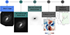Fig. 1.

Workflow showing the different steps involved in this study. From left to right, first, we start from the NIR image from Spitzer. Next, we apply the ICA technique to this image, in order to derive the gravitational potential in the plane of the galaxy (third step). In the fourth step, we compute forces to create a non-weighted torque map. In that image we represent, for clarity, the bar (as a cyan-contoured ellipse) and white contours corresponding to [5σ, 15σ, 45σ, ..., 0.9σ_max] in the CO map, with σ the mean value of the gas map and σ_max its maximum value. Finally, in the fifth step, by weighting the torques by the gas and azimuthally averaging the result, we obtain a torque profile, where we estimate the CR location (pink dot) inside the 0.75R_bar − 2.25R_bar region (green shaded region).

Prior to obtaining the gravitational potential, our images are deprojected according to the PA and i from Table A.1, using the code pydisc⁸ implemented in Python. Readers can refer to Sect. 5.4 to see caveats related to the deprojection process.

3.1. Gravitational potential

Following Binney & Tremaine (1987, Section 2.8), it is possible to obtain the gravitational potential Φ(r) as a convolution of the three-dimensional mass density ρ(r′) and the function 1/r:

$\begin{matrix} Φ (r) = - G \int \frac{ρ (r^{'}) d^{3} r^{'}}{| r - r^{'} |} . \end{matrix}$ $\begin{aligned} \Phi (\mathbf r ) = -G \int \frac{\rho (\mathbf r^{\prime } )d^3\mathbf r^{\prime } }{|\mathbf r -\mathbf r^{\prime } |}. \end{aligned}$ (3)

However, in order to take into account the true three-dimensional mass density, it is necessary to consider the true thickness of the galactic disk. This implicitly assumes that the disk is baryon-dominated, as expected for the inner regions of high surface brightness spiral galaxies (e.g., Kranz et al. 2003), where we have CO observations. However, this can still introduce a bias, which we discuss in Sect. 5.4. To take this thickness into account, we adopt a vertical profile of constant scale-height (see Wainscoat et al. 1989; Barnaby & Thronson 1992):

$\begin{matrix} Φ (x, y, z = 0) = - G \int Σ (x', y') g (x - x', y - y') d x' d y', \end{matrix}$ $\begin{aligned} \Phi (x,y,z = 0) = -G \int \Sigma (x\prime , y\prime ) g(x-x\prime , y-y\prime )\mathrm{d}x\prime \mathrm{d}y\prime , \end{aligned}$ (4)

where g(x, y, z = 0) is the convolution function:

$\begin{matrix} g (x, y, z = 0) = \int_{- \infty}^{\infty} \frac{ρ_{z} (z) d z}{\sqrt{x^{2} + y^{2} + z^{2}}}, \end{matrix}$ $\begin{aligned} g(x,y,z = 0) = \int _{-\infty }^{\infty } \frac{\rho _z(z)\mathrm{d}z}{\sqrt{x^2+y^2+z^2}}, \end{aligned}$ (5)

and, according to Wainscoat et al. (1989) and Barnaby & Thronson (1992), we assume our galaxies have a vertical distribution similar to that of an isothermal disk:

$\begin{matrix} ρ_{z} (z) = ρ_{0} {sech}^{2} (z / h), \end{matrix}$ $\begin{aligned} \rho _z (z) = \rho _0 \mathrm{sech}^2{(z/h)}, \end{aligned}$ (6)

with h proportional to the disk scale-length H_disk as follows:

$\begin{matrix} h \sim 1 / 12 H_{disk}, \end{matrix}$ $\begin{aligned} h\sim 1/12 H_{\rm disk}, \end{aligned}$ (7)

where H_disk is obtained from photometric decompositions of NIR images (Salo et al. 2015; Querejeta et al. 2021). The convolution for the potential is implemented using a Fourier transform approach (see García-Burillo et al. 2005 or Querejeta et al. 2016 for more details).

3.2. Torques

Once the gravitational potential is obtained, the forces can be calculated as the gradient of the gravitational potential in Cartesian coordinates F_x, y(x, y) = − ∇_x, yΦ(x, y). Then, the torques per unit gas mass, in units of km² s⁻², associated with the gravitational potential are obtained as follows:

$\begin{matrix} t (x, y) = x F_{y} - y F_{x} . \end{matrix}$ $\begin{aligned} {t(x,y)} = xF_y - y F_x . \end{aligned}$ (8)

The instantaneous rate of change (gain or loss) of angular momentum experienced by the gas over time, this is, τ = dL/dt, is obtained by multiplying the torque by the total amount of molecular gas in each position.

3.3. Gas flows

The next step consists of using the torque field to derive the angular momentum variations as a function of radius. We assume that the measured CO gas column density, N(x, y), is representative of the locations where gas spends more time as it orbits around the galaxy, this is, we assume steady state. In this statistical approach, we implicitly average over all possible orbits of gaseous particles and take into account the time spent by the gas clouds along the orbit paths. Thus, we compute the azimuthally averaged torques weighted by the present-day gas distribution as in Eq. (9). This is done by an integration of pixels in an annulus defined as [R + δR], where δR = 1.5 arcsec.

$\begin{matrix} τ (R) = \frac{\int_{θ} [N (x, y) \cdot (x F_{y} - y F_{x})]}{\int_{θ} N (x, y)} . \end{matrix}$ $\begin{aligned} \tau (R) = \frac{\int _{\theta } [N(x,y)\cdot (xF_y - y F_x)]}{\int _{\theta } N(x,y)}. \end{aligned}$ (9)

We adopt the convention that negative torques imply gas inflow and positive torques correspond to gas outflow. Thus, the sense of circulation of the gas affects the sign of τ(R). Assuming a dextro-rotatory [x, y, z] reference frame, we need to reverse the sign of τ(R) if the galaxy rotates clockwise, while the sign remains unchanged if the galaxy rotates counter-clockwise. Since all spirals in PHANGS are trailing (see Lang et al. 2020), we assign the corresponding signs based on the orientation of spiral arms (as listed in Table A.1).

The net effect of torques is expected to result in a gas inflow inside CR and outflow immediately outside of it. However, this picture can become more complex if there are additional density wave modes in the disk that compete with the bar potential, which can affect the torque profile around the CR (e.g., García-Burillo et al. 2009; Meidt et al. 2009) and also favor gas inflow inside the ILR region, like the presence of trailing spirals (e.g., Haan et al. 2009; Combes et al. 2014; Audibert et al. 2021).

We identify the CR of the bar at the location where τ(R) changes its sign from negative (R < R_CR) to positive (R > R_CR). As bars are not isolated structures, we expect to find fluctuations in the torque profiles, due to the influence of other components such as spiral arms. This often results in multiple zero crossings, and we identify the most significant crossing as the one with the largest amplitude, which we associate with R_CR. The amplitude is automatically calculated inside a range that spans from the previous to the following crossing (regardless of whether these are negative-to-positive crossings or vice versa). So the amplitude is calculated as $abs (τ_{\max} - τ_{\min})$ $\rm abs({\tau_{\mathrm{max}}-\tau_{\mathrm{min}}})$ , where τ_max is the maximum τ value reached within this range and τ_min the minimum value. This process is repeated for each galaxy. The CR is expected to lie in the radial range defined by R ∼ [R_bar, 2R_bar], where R_bar is obtained from Querejeta et al. (2021). This is because we do not anticipate to find the CR position inside the bar because, at least according to classical theory, stable periodic orbits become chaotic beyond the CR, implying that a bar cannot go beyond this location (Contopoulos & Papayannopoulos 1980; Contopoulos 1980; Elmegreen 1996). The upper limit on this radial range is motivated by the previous findings in the literature, that obtain a mean value for the range of R ≃ (1.5 ± 0.5) R_bar. Moreover, the choice of extending this range much further out than 2R_bar would only be justified in the case of slow bars suspected of having been misclassified by the gravitational torque method. These are, nevertheless, virtually absent in our sample (see Sect. 5.4.5). However, we extend this interval further, from 0.75R_bar to 2.25R_bar, considering that Δ = 0.25R_bar is a reasonable margin given typical uncertainties (discussed in Sect. 3.5).

We assessed the impact of extending the radial range to 0.3R_bar − 2.25R_bar, but this change mainly affects galaxies with a non-robust quality flag QF (i.e., QF = 3, see Sect. 3.5.2). In some particular cases, this change can affect galaxies with robust QF, but after a visual inspection, we believe the selected crossings in these particular cases are artifacts. Therefore, we establish 0.75R_bar − 2.25R_bar as the range in which we search for the CR of the primary bar.

3.4. Identifying other dynamical resonances

We use rotation curves based on CO kinematics from Lang et al. (2020) as a proxy for the circular velocity. These rotation curves approximate the circular velocity v_c in 150 pc wide fixed radial bins. Bayesian Markov Chain Monte Carlo (MCMC) analysis was used to fit the galaxy center, i, and PA. After that, the rotational velocity within a sequence of radial annuli was modeled using harmonic decomposition and least-squares fitting.

The rotation curves from Lang et al. (2020) are defined as the azimuthally averaged tangential velocity of the gas, this is, v_c = ⟨v_θ⟩(R). It is important to note that the epicyclic theory is only valid when the perturbations are small. Thus, the calculated dynamical resonances may not be entirely correct, when studying bars (especially strong ones).

We have tried a number of alternatives (available on Zenodo) before choosing our nominal rotation curves and find significant differences. Thus, we recommend to use the derived Lindblad resonances with care, especially for the cases where the derived rotation curves are subject to large uncertainties.

We can infer other dynamical resonances (such as the Lindblad resonances) using the rotation curve derived from the PHANGS-ALMA observations in Lang et al. (2020). We note that our choice of rotation curves introduces some intrinsic uncertainty in the location inferred for the ILR and OLR. From our derived R_CR, we estimate the pattern speed Ω_p as the intersection of the position of the R_CR and the angular velocity curve, since Ω = v/R, and estimate other important resonances such as the Lindblad resonances.

Apart from CR, using the epicyclic theory, we infer the ILR and OLR. We calculate Ω ± κ/2 curves, where κ is the epicyclic frequency calculated as follows:

$\begin{matrix} κ^{2} = R \frac{d Ω^{2}}{d R} + 4 Ω^{2} . \end{matrix}$ $\begin{aligned} \kappa ^2 = R \frac\mathrm{{d}\Omega ^2}\mathrm{{d}R} + 4 \Omega ^2. \end{aligned}$ (10)

Since for a bar (m = 2), Ω = Ω_p ± κ/2 (Eq. (1)), the intersection of Ω ± κ/2 with the pattern speed Ω_p provides the location of the ILR and OLR, respectively. Thus, the inferred position of ILR and OLR depend on the derivative of the rotation curve, which makes results highly sensitive to local wiggles. Results for all galaxies are listed in Table C.1 and visually shown in the additional material available on Zenodo and in Sect. 4. We note that there are cases where we retrieve two ILR. In those cases we have an inner and outer ILR, designated as iILR, oILR, which leads to an ILR region.

3.5. Uncertainties and quality flags

A change of i, PA or center position may either artificially reinforce or lower the strength of the bar mode present in the disk and/or also introduce “fake” m = 1 terms in the gravitational potential. We estimate the uncertainty and robustness (or QF) of the R_CR via bootstraping.

We derive the nominal CR following the i and PA from Table A.1 (which also shows their uncertainties, which we use for bootstrapping) in addition to the center position and its uncertainty (± 0.5 px). For each iteration, a value of the input parameters is chosen following a Gaussian distribution according to its error bars. Therefore, we obtain a new torque (weighted by the gas) profile in each iteration, for different input parameters, and repeat this process N = 100 times. Figure 2 schematically shows the process.

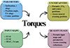Fig. 2.

Schematic diagram that shows the process involved in obtaining CR uncertainties and quantifying QF.

3.5.1. Uncertainties

To estimate the uncertainties in R_CR, we perturb each input parameter (i, PA, center) following a Gaussian distribution within its error bars N = 100 times. For each iteration, we reassess the position of a given CR as the nearest crossing from negative to positive. We take the 16th–84th percentile range on the resulting CR as the error bar (σ_CRⁱ, $σ_{CR}^{PA}$ $\sigma_{\mathrm{CR}}^{PA}$ or $σ_{CR}^{center}$ $\sigma_{\mathrm{CR}}^{\mathrm{center}}$ ). Then we combine all errors by adding them in quadrature as in Eq. (11). The resulting uncertainties are listed in Table B.1.

$\begin{matrix} σ = \sqrt{{(σ_{CR}^{i})}^{2} + {(σ_{CR}^{PA})}^{2} + {(σ_{CR}^{center})}^{2}} . \end{matrix}$ $\begin{aligned} \sigma = \sqrt{\left(\sigma _{\rm CR}^i\right)^2 + \left(\sigma _{\rm CR}^{PA}\right)^2 + \left(\sigma _{\rm CR}^\mathrm{center}\right)^2}. \end{aligned}$ (11)

3.5.2. Quality flags

It is possible that when varying the input i, PA or center position, a different crossing is chosen, in the sense that a different crossing has a larger amplitude from negative to positive torques after perturbing the input parameters. The amplitude of the crossings is automatically calculated inside a range (from the previous to the following crossing) as abs(τ_max − τ_min). Readers can refer to Sect. 3.3 for more details.

Therefore, to assess the crossing robustness, we again perturb each input parameter (i, PA, and center) within their error bars (following a Gaussian distribution) and look for the preferred crossing in each iteration. We note that, when perturbing the parameters, the amplitude of the crossings may change from one iteration to another. Therefore, the chosen crossing in a certain iteration may be different than the nominal one, giving an idea of the robustness of the nominal crossing. As before, the chosen crossing in each iteration is defined as the location in the disk inside the adopted radial range [0.75R_bar, 2.25R_bar] where the negative to positive sign change shows the largest amplitude. This process is repeated N = 100 times for each parameter, taking the 16th-84th percentile range on the resulting CR as the error bar (err_i, err_PA or err_center).

Next, we vary the stellar mass maps and calculate the CR position for each map (ICA1, ICA2 and IRAC, see Sect. 2.3). Once we have the three values for each galaxy, we compare the CR obtained with the nominal map with the other ones and select the maximum difference as the err_map. Once we have errors associated with i, PA, center and stellar mass map variations, we conservatively assume: err = max{err_i, err_PA, err_center, err_mass map}. We do this to showcase the worst-case scenario in terms of the location of the CR, as this procedure will show if the crossing is more sensitive to perturbations in the input parameters. Then we assign QF following the criteria:

$\begin{matrix} If {\begin{matrix} e r r < 30 % R_{bar} ⟹ Q F = 1 \\ 30 % R_{bar} < e r r < 80 % R_{bar} ⟹ Q F = 2 \\ e r r > 80 % R_{bar} ⟹ Q F = 3 . \end{matrix} \end{matrix}$ $\begin{aligned} \text{ If} \ \left\{ \begin{aligned} err < 30 \% \ R_{\rm bar} \Longrightarrow QF = 1 \\ 30 \% \ R_{\rm bar} < err < 80 \% \ R_{\rm bar} \Longrightarrow QF = 2 \\ err > 80 \% \ R_{\rm bar} \Longrightarrow QF = 3. \\ \end{aligned} \right. \end{aligned}$ (12)

Therefore, galaxies with an assigned QF = 1 are the ones that present the most reliable solutions, this is, the negative-to-positive crossing with the largest amplitude remains stable to perturbations of the input parameters within their error bars and to perturbations of the stellar mass maps. The ones with QF = 2 represent intermediate cases, with a slight change in the position of the largest crossing. Finally, the ones with QF = 3 represent the least reliable cases which are excluded from our plots and subsequent calculations. The QF are further validated by visual inspection of the results, as they may eventually depend on other factors such as S/N of CO maps (Sect. 2.2) or insufficient coverage of the bar region (Sect. 2.2). In 21 galaxies (46%) (see Table B.1) we degrade the QF to QF = 3 due to various reasons, such as unreliable or insufficient CO coverage, unreliable radial torque profiles, or the extent of the error bars (see additional material on Zenodo for individual galaxies profiles and explanation of the downgrading). While in one galaxy (2%) we upgrade the QF as we believe both the gas response and stellar potential behave as expected (see additional material).

4. Results

We start by presenting four case studies (Sects. 4.1 to 4.4), before shifting to results on CR based on the whole sample (Sect. 4.5). We choose these four case studies based on their different bar strengths (SAB vs SB), the presence of a nuclear bar (NGC 4321), or the presence of a central ring (NGC 1097), to showcase the connection with the ILR. The number of case studies is chosen to demonstrate how these and other factors cause variations in torque profiles, as well as to have a more comprehensive comparison with the literature. In Sect. 4.5 we also consider other dynamical resonances and compare our results with the literature.

4.1. NGC 1097

Figure 3 shows the torque map and torque profile for NGC 1097. In the central part of this galaxy, we observe the expected butterfly pattern (a change of signs in the bars’ consecutive quadrants). Another butterfly pattern on larger scales beyond the bar has a different orientation. This could be explained by a scenario where the stellar spiral structure has a different pattern speed than the bar (e.g., García-Burillo et al. 2009; Meidt et al. 2009). In this scenario, our profile probes the area inside the CR resonance of the spiral structure. This secondary spiral mode might be characterized by a lower pattern speed and results in negative torques inside the spiral CR. These negative torques can lower the positive torques associated with the bar immediately outside the bar CR. Furthermore, in this map, we can see departures from a smooth map (e.g., dipoles out of the butterfly pattern). These can arise from the imperfect subtraction of dusty regions in the stellar mass map, or from image artifacts that are not properly masked but they should have a limited impact on the torque profiles after azimuthally averaging.

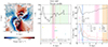Fig. 3.

NGC 1097 (SB) non-weighted deprojected torque map (left panel), torque profile (upper central panel), comparison with values from the literature (lower central panel), rotation curve (upper right panel), and angular rotation curve (lower right panel). The cyan-contoured ellipse in the left panel indicates the bar extent. We show contours corresponding to [5σ, 15σ, 45σ, …, 0.9σ_max] in the CO map, where σ is the mean value of the gas map σ = 0.59 K km s⁻¹, and σ_max = 934.83 K km s⁻¹. In the central and right panels, CR is represented as a vertical pink line, together with its uncertainties (pink-shaded area). This is a statistical uncertainty due to bootstrapping for i, PA and center position (see Sect. 3.5). The solid green line represents the bar length (from Querejeta et al. 2021), while the shaded green region represents the region where we search for the CR. Brown dashed line marks the radius at which the coverage of CO starts to be nonuniform (R_100% CO in Table A.1), orange dashed line is the radius at which the coverage of CO is uniform about 50% (R_50% CO in Table A.1), and purple dashed line represents the end of CO coverage (R_End CO in Table A.1). The shaded gray region represents the inner region inside which we cannot say anything on τ(R) due to the limited spatial resolution of our observations. Finally, in the lower central panel, each dot represents a different measure of the CR (of the main bar) from the literature, and the ⬧ symbol represents a measure of a nuclear bar CR. For both right panels, the solid black line represents the rotation curve (upper panel) and the angular rotation curve Ω (lower panel). Solid light pink and light blue lines represent Ω + κ/2 and Ω − κ/2, respectively. The OLR and its uncertainties are represented in orange and the oILR (and its uncertainties) in dark blue. Purple vertical line represents the central ring detected by Querejeta et al. (2021).

Now, if the gas response is canonical inside (outside) the bar CR, the gas feels negative (positive) torques and as a consequence, the τ(R) profile will show negative (positive) values at R < R_CR (R > R_CR), as shown in the upper central panel of Fig. 3, where we show the azimuthal average torque profile of NGC1097. In the particular case of NGC 1097, we find negative torques along the leading sides of the bar, as expected. In this panel, the change from negative to positive torques at R_CR = 6.4 kpc, is identified as the CR. There are two more crossings from negative to positive within the range where we look for CR, but their overall amplitude is smaller, which is why the first crossing is automatically chosen (as explained in Sect. 3.3). A visual inspection of the profile confirms that weighted torques are clearly negative inside this crossing, as expected inside the bar CR. This figure also contains a comparison with other estimates of the R_CR obtained from the literature using a range of different methods (lower-middle panel), obtaining a reasonable agreement between those values (and their uncertainties) and the one we calculated. In Fig. 3, well inside the CR, we clearly see a second crossing from negative to positive τ(R) at R ∼ 0.7 kpc, which could be indicative of an ILR, and is potentially related to the presence of a ring. Indeed, by visual inspection, we find a ring both in deprojected CO and deprojected 3.6 μm at R ∼ 10.4″ ∼ 0.7 kpc and R ∼ 13.6″ ∼ 0.9 kpc respectively, which is consistent with the results from Comerón et al. (2014), where R_ring = 9.3 − 14.1″ (deprojected).

We note that Font et al. (2014b) identified a secondary inner bar. With our analysis, we tentatively find the signature of the nuclear bar on the sign of the τ(R) profile which switches to negative values for R < 0.7 kpc (see Fig. 3). This is the expected behavior for the torque profile if the gas lies inside the CR of the nuclear bar at these inner radii.

Finally, we measure a pattern speed value of Ω_p = 38.5 ± 4.7 km s⁻¹ kpc⁻¹. This leads to an oILR at R = 1.0 kpc and an OLR at R = 9.6 kpc. When inferring the ILRs, the iILR shows a positive slope in the Ω − κ/2 curve, while the oILR shows a negative slope. This way, we are able to distinguish them. In this particular case, one could argue the iILR should be at R = 1.0 kpc and the oILR at R = 2.0 kpc. However, we believe this is not correct, as this bump in Ω − κ/2 seems to be the result of an artifact in the rotation curve. That is why, when interpreting these results, it is important to keep in mind that the input rotation curves are not circular velocities and that this may have a significant impact on the derived locations of resonances, as seen in some examples in the additional material.

4.2. NGC 3627

Figure 4 shows the torque map, torque profile and rotation curves for NGC 3627. In this figure there are two different butterfly patterns, similar to those in NGC 1097. We distinguish the expected butterfly pattern inside the bar region and a second one on larger scales, which has a different orientation (as explained in Sect. 4.1). As expected, there are negative torques along the leading sides of the bar. Taking a look at this torque profile (upper central panel of Fig. 4), we consider the CR to be at R_CR = 5.2 kpc.

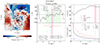Fig. 4.

NGC 3627 (SB) non-weighted deprojected torque map (left panel), torque profile (upper central panel), comparison with values from the literature (lower central panel), rotation curve (upper right panel), and angular rotation curve (lower right panel). We show contours corresponding to [5σ, 15σ, 45σ, …, 0.9σ_max] in the CO map, where σ is the mean value of the gas map σ = 1.21 K km s⁻¹ and σ_max = 1394.02 K km s⁻¹. Symbols as in Fig. 3. The CR is automatically selected as R_CR = 5.2 kpc, due to the change of torques signs at this position and the amplitude of the crossing. R = 3.5 kpc is not selected as the CR because the torque profile does not change sign at this position. R = 6.3 kpc is not selected as the CR because, even though the torque profile changes sign, it oscillates around zero (a behavior usually associated with the presence of a spiral) and presents a lower amplitude (compared to R_CR = 5.2 kpc ).

It can be argued that either the peak at R = 3.5 kpc or the crossing at R = 6.3 kpc are more plausible crossings, however they are not chosen due to various reasons. On the one hand, the peak at R = 3.5 kpc cannot be selected as R_CR because the torque profile does not change sign at this position. On the other hand, the crossing at R = 6.3 kpc could be more plausible, because torques become positive after ∼ 6.3 kpc and, at smaller radii, torques are only mildly positive, with oscillations around zero. However, this behavior could result from the presence of the spiral, which decreases intrinsically positive torques due to the bar. Taking this into account, the selected crossing is R_CR = 5.2 kpc because its amplitude is larger than the amplitude of R = 6.3 kpc. We note that there is also a peak at R ∼ R_bar that approaches zero without crossing. This could be another plausible candidate for the CR. Finally, we measure a pattern speed value of Ω_p = 38.8 ± 1.8 km s⁻¹ kpc⁻¹, leading to an oILR at R = 0.6 kpc and an OLR at R = 6.8 kpc.

4.3. NGC 4321

Figure 5 shows the torque map and torque profile for NGC 4321. A butterfly pattern is clearly visible in the torque map, that alignes quite well with the bar. In addition, inside the bar, we find negative torques along the leading side of the bar edges. Based on the method from García-Burillo et al. (2005), the selected crossing (R_CR = 3.7 kpc ) clearly represents the CR of the bar. However, several literature studies place the CR further out in the disk, and that would be consistent with a coupling of the R_{CR_bar} with the R_{ILR_spiral} or the inner 4:1 resonance of the spiral (Font et al. 2014a). Readers can refer, for example, to Gnedin et al. (1995), that found a peak in the torque profile at R ∼ 11 kpc, in agreement with our profile, and which would almost certainly correspond to the spiral.

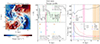Fig. 5.

NGC 4321 (SAB) non-weighted deprojected torque map (left panel), torque profile (upper central panel), comparison with values from the literature (lower central panel), rotation curve (upper right panel), and angular rotation curve (lower right panel). We show contours corresponding to [5σ, 15σ, 45σ, …, 0.9σ_max] in the CO map, where σ is the mean value of the gas map σ = 1.08 K km s⁻¹ and σ_max = 885.64 K km s⁻¹. The teal dashed line represents the nuclear bar radius registered by Querejeta et al. (2021). Symbols as in Fig. 3.

Visually inspecting the central region of the torque profile, we find a clear negative-to-positive crossing at R ∼ 0.6 kpc, leading to gas accumulation between R ∼ 0.6 kpc and R ∼ 1.1 kpc (positive-to-negative crossing), where we expect to find a ring. Indeed, upon visual inspection, we find a ring both in CO and 3.6 μm at R ∼ 7.4″ ∼ 0.5 kpc (CO deprojected) and R ∼ 8.2″ ∼ 0.6 kpc (3.6 μm deprojected), which is coherent with the results from Comerón et al. (2014), where R_ring = 8.2 − 9.0″ (deprojected) and also with the measurements from Querejeta et al. (2021), for which R_inner ring = 8.4″ (deprojected). Finally, we measure a pattern speed of Ω_p = 44.2 ± 4.5 km s⁻¹ kpc⁻¹. We have found an oILR at R = 0.9 kpc and an OLR at R = 7.2 kpc.

4.4. NGC 4579

Figure 6 shows the torque map and profile for NGC 4579, where a butterfly pattern, perfectly aligned with the orientation of the bar, is clearly seen. This states that the large-scale bar dominates the torque field. Inside the bar, we find gas preferentially along the leading edges of the bar, this is, negative torques along this side of the bar.

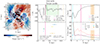Fig. 6.

NGC 4579 (SB) non-weighted deprojected torque map (left panel), torque profile (upper central panel), comparison with values from the literature (lower central panel), rotation curve (upper right panel), and angular rotation curve (lower right panel). We show contours corresponding to [5σ, 15σ, 45σ, …, 0.9σ_max] in the CO map, where σ is the mean value of the gas map σ = 0.56 K km s⁻¹ and σ_max = 258.19 K km s⁻¹. The iILR and its uncertainties are represented in cyan. There is no oILR due to artifacts on the rotation curve. Symbols as in Fig. 3.

For NGC 4579, the torques robustly point to a CR at R_CR = 3.3 kpc because torques are mostly negative at R < 3.3 kpc, even though they oscillate around zero afterwards. As commented before, this could result from the presence of the spiral structure. Most studies from the literature place the R_CR further out, these results could be explained due to the coupling of the R_{CR_bar} with the R_{ILR_spiral}. We note that there is another negative-to-positive crossing at R ∼ 2.5 kpc. This crossing is not selected as the CR, as it is outside the region where we choose to find the CR (0.75R_bar − 2.25R_bar, see Sect. 3.3), even though it is in better agreement with other measurements from the literature (Buta & Zhang 2009; Sierra et al. 2015).

We measure a pattern speed Ω_p = 68.2 ± 3.5 km s⁻¹ kpc⁻¹, and the positions of the iILR and OLR, at R = 0.4 kpc and R = 7.4 kpc, respectively. We note that in this particular case, there is no oILR, due to an artifact in the rotation curve, possibly due to limited CO coverage.

4.5. Statistics

The analysis explained in the previous subsections is carried out for our sample of 46 barred galaxies. Figures analogous to Figs. 3, 4, 5 and 6 for the remaining galaxies can be found in the additional material available on Zenodo. We derived the R_CR for 38 out of 46 galaxies (83% out of the barred sample, Table B.1). For the remaining eight galaxies we did not find a negative-to-positive crossing in the torque profiles within the [0.75R_bar − 2.25R_bar] range (possibly due to limited CO coverage).

As explained in Sect. 3.5.2, we have established automated QF that indicate the reliability of the identified CR. We visually inspected the results and manually downgraded some QF, for example due to limited CO coverage around the identified CR, high i, or insuficient FoV coverage (Table B.1). Out of 46 galaxies, 22 were modified (∼48%): 21 galaxies (∼46%) were downgraded and one galaxy (∼2%) was upgraded. Once this double-check is done, we find that 20 out of 46 barred galaxies are reliable, this is, a 43% of the barred sample have a QF of either QF = 1 (8 galaxies, ∼17%) or QF = 2 (12 galaxies, ∼26%). In Sect. 5.1 we compare our estimations of the R_CR (with QF = 1, 2) with previous estimates, while in Sect. 5.2 we examine the ratio ℛ = R_CR/R_bar.

Finally, knowing the rotation curves for these galaxies, we can obtain the angular rotation curve for each galaxy (see Sect. 3.4). Then, as we have already calculated the CR position (see Table B.1), we can obtain the pattern speed value Ω_p, and the corresponding Lindblad resonances (iILR, oILR, OLR). Table C.1 lists the different pattern speeds and Lindblad resonances found for this sample.

From our sample, we have a total of 19 ILRs (i.e., a 41% of the sample) deduced from the inferred CR (see Table C.1). As discussed in Sect. 3.4, the choice of the rotation curve affects the ILR/OLR calculation, for example some rotation curves lead to a nonexistence of an ILR. In Querejeta et al. (2021), a total of 12 galaxies have a central ring. Therefore, there are five galaxies in common between our sample of ILRs and the subsample of Querejeta et al. (2021) that present a central ring. If we cross-check these two sets, we can check if the central ring lies inside the ILR, as predicted by Sormani et al. (2024)⁹. Examining these five galaxies (NGC 1097, NGC 1300, NGC 2903, NGC 4321 and NGC 5248) we notice that in all these galaxies (100%), the central ring lies inside the registered ILR (see Table 1). In order to double-check these results, we visually obtain the size of the ring in both CO and 3.6 μm images, and also take into account results from Comerón et al. (2014), confirming that the rings form inside¹⁰ the inferred positions of the ILR, in agreement with the expectation from Sormani et al. (2024).

Table 1.

Central ring positions.

5. Discussion

5.1. R_CR comparison

Here we compare our estimations of the R_CR (with QF = 1, 2) with previous estimates from the literature. Figure 7 summarizes these comparisons. We quantify the differences using a Spearman correlation coefficient (see Table 2).

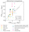Fig. 7.

CR measurements from the literature compared to CR measurements obtained through the gravitational torque method (García-Burillo et al. 2005). Readers can refer to Table 2 for statistics on each method. Vertically aligned data points correspond to the same galaxy presenting different measurements from the literature. References on each method can be found in Table D.1.

Table 2.

Comparison of the methods of the literature.

First we study the relation between our results and the CR measurements (for galaxies with QF = 1, 2) from the literature, without differentiating the various methods, to see in general terms if our results do or do not agree with the literature. We obtain a Spearman coefficient ρ = 0.64 (p-value < 0.001). This pair of values indicates a moderate positive relationship between our CR measurements and the ones from the literature, and a high significance of such correlation. The measurements from the literature are, on average, reasonably coincident with the CR measurements of this paper, as the mean quotient of all datapoints CR_{This paper}/CR_Literature ∼ 0.9 and the median is ∼0.8 (see Table 2). However the scatter among methods (not just with our results) suggests typical uncertainties, in practice, are very large.

We also study the same statistics splitting the literature measurements based on the methods used to obtain the CR measurement, namely: Tremaine-Weinberg (Tremaine & Weinberg 1984a) hereafter TW, offset method (Egusa et al. 2009), phase-reversal method (Font et al. 2011), potential-density phase-shift method (Zhang & Buta 2007; Buta & Zhang 2009), hydrodynamical simulations (such as Garcia-Burillo et al. 1998; Rautiainen et al. 2008), kinematics (such as Chemin et al. 2003; van de Ven & Fathi 2010), morphological methods (such as Buta 1986b; Elmegreen et al. 1996), and gravitational torques (García-Burillo et al. 2005). A comparison of our results to the literature, classified by methods, can be found in Table D.1 while a collection of correlations between all methods is provided in the additional material.

5.1.1. Tremaine-Weinberg method comparison

In general, our measurements agree quite well with the results derived from the TW application. Hereby, we refer to the TW method applied to a particular tracer as TW-tracer, namely: CO (Williams et al. 2021), Hα (Hernandez et al. 2005; Williams et al. 2021), MUSE M_⋆ (Williams et al. 2021). The Spearman coefficient (ρ) yielded a value of 0.89, 0.77, and 0.89 for TW-CO, TW-Hα, and TW-MUSE M_⋆ respectively, indicating a strong positive relationship between the variables. Meanwhile the p-value for each correlation is 0.037, 0.072, and 0.037, indicating quite a high significance. We note that the number of datapoints available for comparison is low¹¹.

The TW methods overestimate by little the CR measurements compared to ours, as CR_This paper/CR_{TW − CO} = CR_This paper/CR_{TW − Hα} ∼ 0.9 and CR_This paper/CR_{TW − MUSE M_⋆} ∼ 0.8. This could be explained based on the third of the three main assumptions of the TW method: the satisfaction of the continuity equation, as this assumption may not be met with the tracers we are working with, namely Hα (Hernandez et al. 2005; Williams et al. 2021) and CO (J = 2 − 1) (Williams et al. 2021). As discussed in Rand & Wallin (2004), the formal validity of this “continuity equation” may be compromised due to the clumpy nature of CO and Hα emissions, as they can introduce fake signals. At high resolution, this effect becomes particularly noticeable when the clumpiness associated with the tracer morphology (CO and Hα) is arranged around specific areas (see Kreckel et al. 2018; Schinnerer et al. 2019; Meidt et al. 2021). This clumpiness may lead to measurements composed of both pattern speed and average velocity field, this is, an overestimated pattern speed value, as shown in Williams et al. (2021) and Borodina et al. (2023). We note that Williams et al. (2021) already reports that using CO and Hα as tracers may not be reliable when applying TW. However, Hernandez et al. (2005) states that the stellar population (e.g., using MUSE stellar mass surface density from Williams et al. 2021 as a tracer) may satisfy the continuity equation, as long as the star formation efficiency is low. We note that in this analysis, NGC 3627 has not been taken into account¹².

5.1.2. Offset method comparison

The offset method consists of using different tracers of gas and star formation along spiral arms in order to calculate Ω_p. These offsets vary radially as a result of the local difference between Ω and Ω_p.

When comparing with the measurements obtained from the application of the offset method (Sierra et al. 2015), we see that their measurements exhibit limited agreement with our results. While ρ = 0.5 indicates a positive relationship, the p-value of 0.667 suggests that the trend is not statistically significant (due to the small number of datapoints: only three). This method tends to underestimate the CR compared to our results, as CR_This paper/CR_Offset ∼ 2.6, as seen in Table 2. The difference between our results and the offset estimations could be due to various reasons. On the one hand, as explained in Sect. 5.4, the deprojection step is crucial, and dependent on the i values, which are not identical to ours. Sierra et al. (2015) obtain a range of i for each galaxy, which differ a lot from the i from Lang et al. (2020). On the other hand, for three out of four galaxies, Sierra et al. (2015) give two values of CR, as there are two nearby crossings (< 5″) and they cannot differentiate between them; in two cases (NGC 4548, NGC 4654) we have adopted the mean value as the CR estimation.

5.1.3. Potential-density phase-shift method comparison

The potential and density spirals are azimuthally shifted form each other. This method assumes the CR to be at the location where the phase shift changes (Zhang & Buta 2007).

The CR estimations derived from the potential density phase-shift method (Zhang & Buta 2007; Buta & Zhang 2009) on average coincide with our CR calculations, as CR_This paper/CR_{PD phase − shift} ∼ 0.9. We find a strong and statistically significant correlation (ρ = 0.83, p-value < 0.001). The potential density phase-shift method (Zhang & Buta 2007) relies on the morphological evidence in H-band images that have been deprojected and decomposed assuming a spherical bulge. The main idea is that the sense of angular momentum exchange between a density wave mode and the fundamental state of a galaxy is indicated by the sign of the phase-shift, which has to change at the CR of the bar, where the phase-shift changes from positive to negative. Even though the assumption of a spherical bulge could lead to what Buta & Zhang (2009) call a “decomposition pinch” (isophotes showing a pinched shape in a deprojected image), they prove the assumption of a spherical bulge does not lead to the presence of a false positive-to-negative crossing. Moreover, the main assumption of this approach is that the wave modes are quasi-steady. If this assumption is not satisfied, the phase-shift plot will be more noisy, and thus the R_CR measurement will not be reliable.

5.1.4. Hydrodynamical simulations comparison

Now, turning our attention to the comparison with hydrodynamical (HD) simulation measurements, we observe that their results tend to be overestimated compared to our results (CR_{This paper}/CR_HD ∼ 0.6). We find a strong and statistically significant correlation (ρ = 0.67, p-value = 0.034). It is important to take into account that in most of these references they first calculate the pattern speed from their model, and only then they can calculate the CR using the modeled rotation curve. This indirect measurement of the CR is very sensitive to changes in the used rotation curve (as seen in Sect. 5.3). Furthermore, for the galaxy NGC 4321, they might be obtaining the CR of the spiral instead of the CR of the bar (Garcia-Burillo et al. 1998).

5.1.5. Kinematics methods comparison

The CR estimations from methods involving kinematics on average coincide with our results, as CR_{This paper}/CR_Kinematics ∼ 0.9. These methods measure R_CR by first deriving Ω_p, and from this value (knowing or deriving the rotation curve) calculating R_CR (Chemin et al. 2003; Hirota et al. 2009; van de Ven & Fathi 2010; Piñol-Ferrer et al. 2014). However, it is important to note that Chemin et al. (2003) and van de Ven & Fathi (2010) combine photometric information with kinematic information, this is, they assume a certain structure of the galaxy corresponds to a dynamical resonance, and from there they obtain Ω_p with the rotation curve. We obtain a Spearman coefficient of ρ = 0.79 and an associated p-value = 0.059 which imply a positive irrelevant correlation between both datasets. The differences between our results and the measurements from the literature involving kinematical methods may rely on the differences on the chosen rotation curves because, as explained in Sect. 5.3, the calculated resonances (including the CR) are very sensitive to the differences between rotation curves.

5.1.6. Phase-reversal method comparison

Following another kinematic approach, the phase-reversal method (Font et al. 2011) overestimates the CR position compared to our results (CR_This paper/CR_{Phase − reversal} ∼ 0.8). We find a moderate correlation between our measurements and the phase-reversal method, even though its statistical significance is marginal (ρ = 0.69, p-value = 0.085). The phase-reversal approach involves determining the galactocentric radius at which a 180° phase shift in the gas response is observed, this is, a phase-reversal. This way, plotting (in histogram format) the phase-reversals of the noncircular velocities as a function of galactocentric radius, the CR can be identified as the strongest “peak” (located near the end of the bar) in this radial distribution histogram, assuming that streaming velocities change sign at the CR. This method requires sufficient resolution and good azimuthal coverage (Font et al. 2014b).

5.1.7. Gravitational torque method comparison

Now, comparing our CR measurements with the literature, where gravitational torques have also been used, we observe that, on average, the results are coincident as CR_{This paper}/CR_Torques ∼ 1.0. However, calculating the Spearman correlation coefficient, we obtain ρ = −0.87 and its associated p-value = 0.333, which are results that imply a strong negative and unreliable correlation, due to the low number of available datapoints (only three reliable datapoints). We note that in this particular case, we do not take into account galaxy NGC 5248, as in Haan et al. (2009) they refer to this CR as related to the “outer spiral/bar”. Therefore, the number of datapoints we use in this comparison is three. García-Burillo et al. (2009) used CO(2-1), CO(1-0) and HI maps to study gravitational torques. Comparing their CR measurements for NGC 4579 with ours we find different torque profiles, this could be the reason of the difference between both measurements. On the other hand, Haan et al. (2009) also used CO(2-1), CO(1-0) and HI maps. They used CO until R ∼ 0.8 kpc and HI from R ∼ 0.8 kpc until R ∼ 6 kpc. Comparing their NGC 3627 results with ours, we see a good agreement. We also realize that following our procedure applied to their torque profiles, we would obtain the CR near the bump mentioned in Sect. 4.2. Finally, in Casasola et al. (2011) they used CO(2-1) and CO(1-0) maps for NGC 3627. Again, we find a good agreement between torque profiles, but their selected CR is related to the bump we find in our torque profiles (which is not our CR).

5.1.8. Morphological method comparison

Examining an alternative approach, we classified as “morphological” methods those that identify stellar structures such as rings, associate them with ILRs, and then calculate the CR position based on such assumption. This approach tends to overestimate the CR calculations according to our results (CR_This paper/CR_Morphology ∼ 0.5). We find a weak and insignificant negative correlation (ρ = −0.07, p-value = 0.899). Differences can be attributed to the choice of rotation curve, as this method critically depends on that measurement, as they assume that the central ring lies at the ILR, they calculate the CR based on that pattern speed (see Sect. 5.3).

5.2. Fast and slow bars

Following Debattista & Sellwood (2000) we classify bars according to ℛ as follows:

$\begin{matrix} \begin{matrix} R < 1, Ultra-fast bars \\ 1 < R < 1.4, Fast bars \\ R > 1.4, Slow bars \end{matrix} . \end{matrix}$ $\begin{aligned} \left. \begin{aligned} \mathcal{R} <1, \ \text{ Ultra-fast} \text{ bars}\\ 1<\mathcal{R} < 1.4, \ \text{ Fast} \text{ bars} \\ \mathcal{R} >1.4, \ \text{ Slow} \text{ bars} \\ \end{aligned} \right. . \end{aligned}$ (13)

We calculate the ratio ℛ = R_CR/R_bar, using the R_bar values compiled by Querejeta et al. (2021). Our average value, if we exclude those galaxies with QF = 3, is ℛ ∼ 1.12 ± 0.39, which is in agreement with the value from Athanassoula (1992): ℛ = 1.2 ± 0.2. Figure 8 shows that most bars are indeed fast, or compatible with the fast region within uncertainties. In this reduced sample of 20 galaxies (only taking into account galaxies with QF = 1, 2) we find six galaxies (30%) presenting fast bars, four galaxies (20%) presenting slow bars and ten galaxies (50%) presenting ultra-fast bars, but in six cases, these galaxies are close to the transition line between these two regimes of ℛ ∼ 1. This is in line with previous findings that bars in the local universe are predominantly fast (e.g., Corsini 2011; Aguerri et al. 2015; Guo et al. 2019; Cuomo et al. 2021 using the TW method), which would argue against the braking of bars by dark matter haloes. Interestingly, the vast majority of measurements quite closely follow the one-to-one line in Fig. 8. This suggests that, to first order, CR lies at the end of the bar for most galaxies and we can estimate the bar pattern speed as Ω_p = Ω(R_bar). There are only a handful of galaxies with clearly higher ℛ, which drive the average close to the standard ℛ = 1.2 value. A graphic analog to Fig. 8 for QF = 1, 2, 3 can be found in the additional material.

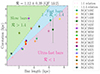Fig. 8.

Slow, fast, and ultra-fast bars containing exclusively galaxies with QF = 1 and QF = 2. Galaxies with QF = 2 are represented with stars, while galaxies with QF = 1 are represented with dots.

Contopoulos & Papayannopoulos (1980) and Contopoulos (1980, 1981) argue against the existence of ultra-fast bars (ℛ < 1) because stable periodic orbits beyond CR become chaotic, implying that a self-consistent bar cannot go beyond its own CR. However, the existence of this kind of bars might be possible in the framework of the manifold theory (Romero-Gómez et al. 2006, 2007; Athanassoula et al. 2009b,a, 2010). While we find several ultra-fast bars in our sample, these lie relatively close to the transition region, and given the large error bars, most of these do not necessarily pose a challenge to the classical theory.

The existence of fast and slow bars has cosmological consequences, as for the braking of bars over time (Debattista & Sellwood 2000. The dynamical friction with the dark matter (DM) halo (Tremaine & Weinberg 1984b; Chiba 2023) can reduce the Ω_p of the bar without increasing its length (Debattista & Sellwood 2000), causing the CR to move outward (higher ℛ). However, we find a mean ℛ = 1.12 ± 0.39, this is, a majority of fast bars. The fact that galaxies with fast bars are more common than the ones with slow bars (see also Corsini 2011; Aguerri et al. 2015; Guo et al. 2019; Cuomo et al. 2021; Garma-Oehmichen et al. 2022), could suggest that bars do not suffer much dynamical friction produced by DM haloes, as explained by Fragkoudi et al. (2021), and therefore DM haloes are not likely to be dominant in the inner regions of galaxies. Alternatively, our results might imply that bars do slow down via dynamical friction but at the same time grow in mass and length over time, therefore evolving with ℛ ∼ 1 (Athanassoula 2003).

It is important to note that recent studies such as Font et al. (2017) argue that bars with ℛ < 1.4 might be rotating slower than previously thought because the bar grows faster than the CR moves outward when evolving. So the bars traditionally called “fast” are not necessarily the fastest bars in absolute terms (bars with a larger ℛ can be faster if their bar length is smaller). Therefore, Font et al. (2017) propose to use the bar pattern speed relative to the angular velocity of the disk in order to describe fast and slow rotating bars instead of using ℛ. However, in this paper we follow the traditional nomenclature mentioned above (Eq. (13)).

5.3. Derivation of Lindblad resonances

Central rings have traditionally been associated with the ILR. The simplest line of thought is that rings are formed at the Lindblad resonances (central rings at ILRs and outer rings at OLRs) because, under the constant influence of gravity torques from the bar potential, gas accumulates in such locations (Schwarz 1981; Combes 1988, 1996; Buta & Combes 1996). However, there are alternative models. For example, Sormani et al. (2024) propose that central rings are instead an accumulation of gas at the inner edge of a gap in the gas disk formed around the ILR. This gap develops around the ILR because a bar potential produces the excitation of waves, which remove angular momentum from the gas disk, transporting it inward, and thus forming the ring at the inner edge of the gap. In this framework, the size of the central ring is related to the local sound speed. Moreover, this approach is compatible with rings being inside the ILR, as seen in simulations (Englmaier & Gerhard 1997; Patsis & Athanassoula 2000; Kim et al. 2012; Sormani et al. 2015a; Li et al. 2015).

As seen in Sect. 4.5, for the five galaxies¹³ that present both an iILR/oILR and a ring (as compiled in Querejeta et al. 2021), the central ring lies inside the iILR/oILR we obtain (see Table 1). This also happens when visually obtaining the size of the ring in both CO and 3.6 μm images, and when comparing to the results from Comerón et al. (2014). This agreement confirms that the rings in our reduced sample lie inside the iILR/oILR, as expected from Sormani et al. (2024).

As already mentioned in Sect. 3.4, we expect the identification of resonances to be sensitive to our choice to use the observed rotation velocity curve as a tracer of the circular velocity. This approach follows Lang et al. (2020), and is based on a spline fitting to these CO-based rotation curves (Sun et al. 2020). However, circularity may not always be maintained, as there are local wiggles (e.g., in the case of bar streaming motions or in the centers of galaxies, as seen in Hayashi & Navarro 2006) which can originate from streaming motions, and which can therefore bias the derived Lindblad resonances. In addition, as this is a first-order approximation, we use the observed velocity profile as a proxy for the galaxy’s real circular motion. The observed velocity profile will overestimate the true circular velocity where the non-axisymmetry of the potential predominates, leading to resonance locations that may not be correct. The resonance identification will thus also be sensitive to the chosen rotation curve and its behavior (see Sect. 3.4).

5.4. Methodological choices and caveats

5.4.1. Choice of gas tracer

We favor strict mask maps over the “broad” masks (see Sect. 2.2), which have high completeness at the expense of higher noise, because noise spikes often bias the azimuthal averages when calculating torque profiles. Also we note that in this analysis, we neglect HI because gas is mostly molecular in the inner parts of galaxies, where bars exist. But also, for practical reasons, because we do not yet have HI observations at sufficiently high resolution for this sample of galaxies. We expect this choice to have a limited impact on our results.

5.4.2. α_CO and M/L

The α_CO conversion factor is known to significally depend on metallicity (Bolatto et al. 2013), implying that α_CO changes between galaxies. There is not strong evidence that α_CO varies azimuthally. While arm-to-interarm metallicity variations have been found in some galaxies to be typically on the order of ∼0.05 dex in 12 + log(O/H) (e.g., Ho et al. 2017, 2018), in other cases such arm-to-interarm variations were found to be even more limited or absent (e.g., Kreckel et al. 2019). However, by definition (see Eq. (9)), our results are not going to be affected by radial variations of α_CO or R₂₁, and would only be affected by azimuthal variations, which are expected to be very limited, or at least much more limited than any radial dependencies (den Brok et al. 2021; Leroy et al. 2022).

Another caveat is that, in this analysis, we assume a constant stellar M/L. The M/L is expected to display some radial variations, with much more limited azimuthal trends (e.g., Leroy et al. 2019). Thus, radial variations could affect the relative normalization of the torque profiles, and have an impact on inferred gas inflow rates. Since we do not calculate gas inflow rates in this paper, we expect variations of M/L to have a limited impact on our results.

5.4.3. Deprojection issues

When deprojecting the 2D stellar and gas maps, we assume that any central structures are as flattened as the disk. Therefore, we do not account for spherical bulges, which would result in an unrealistic elongated structure (similar to a bar) after deprojection. This deprojection effect is more critical when working with objects whose i is large. For some galaxies, this deprojection effect may imply an overestimation of the radial forces by a factor of up to two (see Buta & Block 2001). However, this is likely not a large concern, as bulges in PHANGS galaxies are expected to be rather pseudo-bulges, and therefore mostly flat (Querejeta et al. 2021).

5.4.4. Other assumptions

When using the gravitational torque method, we do not take into account the inclusion of gas self-gravity. This effect could produce perturbations that could induce a departure from axisymmetry. However, it is more important at high redshifts, where galaxies contain higher gas fractions.

As seen in Sect. 3.1, a constant scale-height is adopted for each galaxy, to take into account the thickness of the disk when calculating the gravitational potential. Even though the scale-height can affect the derived forces, its effect is negligible, as seen in Querejeta et al. (2016) for M 51, and it mostly affects the scale of the profiles, not the location of the CR. The existence of a Boxy/Peanut (B/P) bulge can be taken into account through the scale-height function. However, we assume there are no B/P bulges, which has an impact on potential forces and bar strengths (e.g., Fragkoudi et al. 2015; Tahmasebzadeh et al. 2021), as this is beyond the scope of the present paper.

We are implicitly assuming that the disks from our sample are baryon-dominated, as we derived the potential from NIR images without accounting for DM. This assumption does not present an issue because DM is expected to be considerably more axisymmetric than the baryonic component studied here. So, if DM were to be dominant, its effect would only change the amplitude of the torque profiles, not the locations at which they change signs. Furthermore, we only study regions where we have a full azimuthal CO coverage, typically excluding the outskirts of galaxies where DM dominates. Yet, our profiles in some cases go out to radii where the contribution from DM might not be negligible. However, as mentioned before, the inclusion of an axisymmetric DM halo when computing the torque profiles will only affect the amplitude of the torques, but not their sign.

Also, as seen in Verwilghen et al. (2024), it appears that gas bars are mostly occurring in galaxies with M_⋆ ≲ 10¹⁰ M_⊙, while more defined bars (and structures such as bar lanes or rings) are formed in more massive galaxies. So there could be an observational bias, as most of our work is focused on more massive galaxies (78.26% of the sample, 36 galaxies).

Another limitation comes from the assumption that the gas response to the stellar potential is roughly stationary with respect to the potential reference frame during a few rotation periods. In order to have a representative gas response for the dynamical resonances, we implicitly average over all orbits of gas at each position and account for the time spent by the gas clouds along all the possible orbit paths rather than following particles along individual orbits. In other words, we assume that the potential does not change much over time. This is a resonable assumption for isolated galaxies (García-Burillo et al. 2009), but could be compromised for interacting systems, where dynamical timescales are shorter.

5.4.5. Determining R_CR in slow bars: Caveats on the use of the torque method

Slow bar candidates identified by the gravitational torque method represent a small percentage of the galaxies analyzed in this paper: only four out of 20 galaxies with QF = 1, 2 in our sample appear to host slow bars. This result is consistent with previous work using alternative observational methods to determine the ℛ parameter in different galaxy samples (Aguerri et al. 2015; Cuomo et al. 2019, 2020). On the other hand, evidence found in different numerical simulations suggests that a significant fraction of barred galaxies should show slow bars (Algorry et al. 2017; Roshan et al. 2021). Fast bars are expected to live in baryon-dominated disks, whereas slow bars could experience a significant drag from the dynamical friction due to a dense DM halo (Buttitta et al. 2022). The small fraction of slow bars identified in observations has been interpreted as being due to the low concentration of DM halos (Debattista & Sellwood 2000) or to the inefficient angular momentum exchange with this component, which is unable to reduce the pattern speed of bars in real galaxies as a result of secular evolution (Athanassoula 2002, 2014). Alternatively, the disagreement between observations and simulations could be explained if observational methods were somehow systematically biased against the detection of slow bars. Also we note that QF = 3 denotes the CR is not reliable, including the cases in which a bar may have been misclassified into a fast or ultra-fast bar, instead of a slow one.

Next we explore the validity of the gravitational torque method used in this work. Combes & Elmegreen (1993) analyzed the expected gas response to a slow stellar bar using self-consistent numerical simulations. In particular, Combes & Elmegreen (1993) studied bar formation and pattern speeds in galaxies with different bulge-to-disk mass ratios. Slow bars form in galaxies with low bulge-to-disk mass ratios, typical of late Hubble-type disks, which have low values of Ω − κ/2 everywhere and correspondingly low bar pattern speeds. In our sample, we have few late Hubble-type galaxies. CR is pushed well beyond the ends of the slow stellar bars, which can only grow up to their ILR. The characteristic gas response to a slow stellar bar consists of a small-scale gas bar that extends to the ILR. Outside the gas bar, a two-armed spiral pattern develops between the ILR and the CR of the bar. For large values of ℛ, the slow bar is therefore substantially shorter than its R_CR, and the offset dust lane gas response inside the bar, characteristic of fast bars, disappears (see also Collier et al. 2018). The gravitational torques exerted on the gas by a slow bar are expected to be negative inside the ILR. On the other hand, the torques between the ILR and the CR of a slow bar are expected to be positive: the two-armed gas spiral lies in the quadrants where the bar-driven torques are expected to be positive. The spiral torques are also expected to be positive in the gas outside the ILR, as the gas in these regions appears systematically upstream relative to the stellar arms. This is in stark contrast to the radial trend pattern expected for the torques in the fast bar scenario, where τ(R) < 0 systematically within R_CR and down to the ILR locus.

The validity of the torque diagnostic tool used in this paper is based on the fact that the CR of the bar defines the transition from negative (τ(R) < 0, R ≤ R_CR) to positive (τ(R) < 0, R ≥ R_CR) torques in the disk. Overall, while this is true for ultrafast, fast and moderately fast bars where ℛ ≤ 1.4, our method may misidentify the ILR of a slow bar as the CR locus. We have investigated the existence of potentially misidentified CR loci among the galaxies in our sample on a case-by-case basis. We suspect that this may be the case in galaxies that have a CO bar within the stellar bar, with no offset CO gas/dust lanes and no conspicuous nuclear gas ring morphology. These cases correspond to galaxies with a smooth Ω − κ/2 curve without a pronounced maximum in the nuclear region. The result of this analysis shows that CR may have been incorrectly assigned by the torque method in virtually none of the galaxies of our sample satisfying that QF = 1, 2. In sum, none of the galaxies suspected to have been misclassified as fast bars passed the QF test (QF < 3).

5.4.6. Rotation curves

As explained in Sect. 3.4, the rotation curves from Lang et al. (2020) are defined as v_c = ⟨v_θ⟩(R). In simulations, the rotation curves are usually defined as $v_{c} = \sqrt{R \cdot d Φ (R) / d R}$ $v_c=\sqrt{R\cdot \rm{d}\Phi(R)/\rm{d}R}$ where Φ(R) is the axisymmetrized gravitational potential (used for example in Sormani et al. 2024). For an ideal case in an axisymmetric gravitational potential, the results from both approaches are essentially the same. However, when working with real observational data, inferring v_c from the gravitational potential relies on strong assumptions and is more indirect than estimating the rotation curve directly from kinematic CO data, despite possible biases introduced, for example, by streaming motions. Given the high-quality of the CO kinematic information available in PHANGS, we prefer to use Lang et al. (2020) rotation curves, but we note that other definitions of v_c could lead to differences in the measurements. Also we note that, strictly speaking, the epicyclic theory is only valid when the perturbations (departures from axisymmetry) are small, therefore it might fail when calculating dynamical resonances associated to a strong bar.

6. Summary and conclusions

We studied a sample of 46 barred galaxies (from the parent sample PHANGS-ALMA, of 74 galaxies) with the gravitational torque method (García-Burillo et al. 2005). We estimated the position of the dynamical resonance of CR by studying the gravitational torques imprinted by the stellar bar on the gas. We examined gravitational torques τ(R) along the galactocentric radius and assumed that the R_CR must be inside the 0.75R_bar − 2.25R_bar range, and that it must be seen as a negative-to-positive crossing in τ(R).

We present here an unprecedented catalog of resonances obtained through the gravitational torque method, containing the bar CR of 38 galaxies out of the 46 barred galaxies analyzed. In this catalog, we include the uncertainties in the CR resonance of the bar, as well as the QF assigned to each galaxy, as a marker of the reliability of the results. We also present in this catalog other interesting dynamical resonances (ILR, OLR), but these must be taken carefully, as they are dependent of the chosen rotation curves. Along with this resonances catalog, we present an inspection and comparison of the bar R_CR present in the literature. After this extensive literature research (ten different methods, 33 different papers), we generally find a good agreement between our CR measurements and the ones calculated in the literature (ρ = 0.64, p-value < 0.001). However, it is important to note that the uncertainties in the CR literature measurements are very large. We also find that our results are most compatible with those from the literature that are calculated using the potential-density phase-shift method.

Once the value of the R_CR is known, and also the approximate R_bar, we calculated the ratio between those two quantities, ℛ = R_CR/R_bar, obtaining an average value of ℛ = 1.12 ± 0.39 (fast bars) when studying the more reliable portion of the sample (i.e., QF = 1, 2). While doing the statistical study, we also classify our sample into galaxies with slow bars, fast bars, and ultra-fast bars. Most of the galaxies from our sample present fast and ultra-fast bars in the region of transition from fast to ultra-fast bars (i.e., ℛ ∼ 1).

Data availability

Supplementary material is available at: https://zenodo.org/records/13898598

¹

m = 2 for a bar, and in that case, l = 1 in the case of the outer Lindblad resonance (OLR), l = −1 in the case of the inner Lindblad resonance (ILR), and l = 0 for the CR.

²

Physics at High Angular resolution in Nearby GalaxieS; http://www.phangs.org

³

Spitzer Survey of Stellar Structure in Galaxies, https://irsa.ipac.caltech.edu/data/SPITZER/S4G/overview.html

⁴

Barred galaxies of type SAB̲ have been classified as SAB.

⁵

Infrared Array Camera.

⁶

Infrared Science Archive.

⁷

Spitzer Infrared Nearby Galaxies Survey.

⁸

https://github.com/emsellem/pydisc

⁹

Note that the rotation curves we are using are defined as v_c = < v_Φ>, while the approach followed by Sormani et al. (2024) defines rotation curves as $v_{c} = \sqrt{R \cdot d Φ / d R}$ $v_c=\sqrt{R\cdot \rm{d}\Phi/\text{ d}R}$ .

¹⁰

For NGC 1097, the ring forms at R_ring ∼ 0.47R_ILR; for NGC 1300 inside the R_ring ∼ 0.29R_ILR; for NGC 2903 inside the R_ring ∼ 0.43R_ILR; for NGC 4321 inside the R_ring ∼ 0.69R_ILR and for NGC 5248 inside the R_ring ∼ 0.57R_ILR.

¹¹

Five datapoints for TW-MUSE M_⋆, and 11 datapoints for gaseous tracers (five measurements for TW-CO, and six measurements for TW-Hα).

¹²

In the case of NGC 3627, the R_CR value from Williams et al. (2021) is far inside the bar, which could be related to rotation curve issues.

¹³

NGC 1097, NGC 1300, NGC 2903, NGC 4321 and NGC 5248.

Acknowledgments

We thank the anonymous referee for carefully reviewing this paper. This work was carried out as part of the PHANGS collaboration. MRG, MQ and SGB acknowledge support from the Spanish grant PID2022-138560NB-I00, funded by MCIN/AEI/10.13039/501100011033/FEDER, EU. MCS acknowledges financial support from the European Research Council under the ERC Starting Grant “GalFlow” (grant 101116226). ES acknowledges funding from the European Research Council (ERC) under the European Union’s Horizon 2020 research and innovation programme (grant agreement No. 694343). ZB gratefully acknowledges the Collaborative Research Center 1601 (SFB 1601 sub-project B3) funded by the Deutsche Forschungsgemeinschaft (DFG, German Research Foundation) – 500700252. RSK acknowledges financial support via the ERC Synergy Grant “ECOGAL” (project ID 855130), from the German Excellence Strategy via the Heidelberg Cluster of Excellence (EXC 2181 - 390900948) “STRUCTURES”, and from the German Ministry for Economic Affairs and Climate Action in project “MAINN” (funding ID 50OO2206). RSK is grateful for computing resources provided by the Ministry of Science, Research and the Arts (MWK) of the State of Baden-Württemberg through bwHPC and the German Science Foundation (DFG) through grants INST 35/1134-1 FUGG and 35/1597-1 FUGG, and also for data storage at SDShd funded through grants INST 35/1314-1 FUGG and INST 35/1503-1 FUGG. RSK also thanks the 2024/25 Class of Radcliffe Fellows for highly interesting and stimulating discussions. AKL gratefully acknowledge support from NSF AST AWD 2205628, JWST-GO-02107.009-A, and JWST-GO-03707.001-A and gratefully acknowledges support by a Humboldt Research Award. SKS acknowledges financial support from the German Research Foundation (DFG) via Sino-German research grant SCHI 536/11-1. PSB acknowledges support from the Spanish grant PID2022-138855NB-C31, funded by MCIN/AEI/10.13039/501100011033/FEDER, EU. This paper makes use of the following ALMA data: ADS/JAO.ALMA#2012.1.00650.S, ADS/JAO.ALMA#2013.1.00803.S, ADS/JAO.ALMA#2013.1.01161.S, ADS/JAO.ALMA#2015.1.00121.S, ADS/JAO.ALMA#2015.1.00782.S, ADS/JAO.ALMA#2015.1.00925.S, ADS/JAO.ALMA#2015.1.00956.S, ADS/JAO.ALMA#2016.1.00386.S, ADS/JAO.ALMA#2017.1.00886.L, ADS/JAO.ALMA#2018.1.01651.S. ALMA is a partnership of ESO (representing its member states), NSF (USA) and NINS (Japan), together with NRC (Canada), MOST and ASIAA (Taiwan), and KASI (Republic of Korea), in cooperation with the Republic of Chile. The Joint ALMA Observatory is operated by ESO, AUI/NRAO and NAOJ. The National Radio Astronomy Observatory is a facility of the National Science Foundation operated under cooperative agreement by Associated Universities, Inc.

References

Aguerri, J. A. L., Méndez-Abreu, J., Falcón-Barroso, J., et al. 2015, A&A, 576, A102 [NASA ADS] [CrossRef] [EDP Sciences] [Google Scholar]
Algorry, D. G., Navarro, J. F., Abadi, M. G., et al. 2017, MNRAS, 469, 1054 [Google Scholar]
Anand, G. S., Lee, J. C., Van Dyk, S. D., et al. 2021, MNRAS, 501, 3621 [Google Scholar]
Athanassoula, E. 1992, MNRAS, 259, 345 [Google Scholar]
Athanassoula, E. 2000, ASP Conf. Ser., 221, 243 [NASA ADS] [Google Scholar]
Athanassoula, E. 2002, ApJ, 569, L83 [NASA ADS] [CrossRef] [Google Scholar]
Athanassoula, E. 2003, MNRAS, 341, 1179 [Google Scholar]
Athanassoula, E. 2014, MNRAS, 438, L81 [Google Scholar]
Athanassoula, E., Romero-Gómez, M., Bosma, A., & Masdemont, J. J. 2009a, MNRAS, 400, 1706 [NASA ADS] [CrossRef] [Google Scholar]
Athanassoula, E., Romero-Gómez, M., & Masdemont, J. J. 2009b, MNRAS, 394, 67 [NASA ADS] [CrossRef] [Google Scholar]
Athanassoula, E., Romero-Gómez, M., Bosma, A., & Masdemont, J. J. 2010, MNRAS, 407, 1433 [NASA ADS] [CrossRef] [Google Scholar]
Audibert, A., Combes, F., García-Burillo, S., & Dasyra, K. 2021, Proc. Int. Astron. Union, 359, 307 [NASA ADS] [Google Scholar]
Balbus, S. A., & Hawley, J. F. 1998, Rev. Mod. Phys., 70, 1 [Google Scholar]
Barnaby, D., & Thronson, H. A., Jr 1992, AJ, 103, 41 [NASA ADS] [CrossRef] [Google Scholar]
Binney, J., & Tremaine, S. 1987, Galactic Dynamics (Princeton, N.J: Princeton University Press) [Google Scholar]
Bolatto, A. D., Wolfire, M., & Leroy, A. K. 2013, ARA&A, 51, 207 [CrossRef] [Google Scholar]
Borodina, O., Williams, T. G., Sormani, M. C., Meidt, S., & Schinnerer, E. 2023, MNRAS, 524, 3437 [NASA ADS] [CrossRef] [Google Scholar]
Buta, R. 1986a, ApJS, 61, 609 [NASA ADS] [CrossRef] [Google Scholar]
Buta, R. 1986b, ApJS, 61, 631 [Google Scholar]
Buta, R. J. 2017, MNRAS, 470, 3819 [Google Scholar]
Buta, R., & Block, D. L. 2001, ApJ, 550, 243 [Google Scholar]
Buta, R., & Combes, F. 1996, Fund. Cosmic Phys., 17, 95 [Google Scholar]
Buta, R. J., & Zhang, X. 2009, ApJS, 182, 559 [Google Scholar]
Buta, R., Ryder, S. D., Madsen, G. J., et al. 2001, AJ, 121, 225 [Google Scholar]
Buta, R. J., Sheth, K., Athanassoula, E., et al. 2015, VizieR Online Data Catalog, J/ApJS/217/32 [Google Scholar]
Buttitta, C., Corsini, E. M., Cuomo, V., et al. 2022, A&A, 664, L10 [NASA ADS] [CrossRef] [EDP Sciences] [Google Scholar]
Canzian, B. 1993, ApJ, 414, 487 [NASA ADS] [CrossRef] [Google Scholar]
Casasola, V., Hunt, L. K., Combes, F., García-Burillo, S., & Neri, R. 2011, A&A, 527, A92 [NASA ADS] [CrossRef] [EDP Sciences] [Google Scholar]
Chemin, L., Cayatte, V., Balkowski, C., et al. 2003, A&A, 405, 89 [NASA ADS] [CrossRef] [EDP Sciences] [Google Scholar]
Chiba, R. 2023, MNRAS, 525, 3576 [NASA ADS] [CrossRef] [Google Scholar]
Colina, L., & Wada, K. 2000, ApJ, 529, 845 [NASA ADS] [CrossRef] [Google Scholar]
Collier, A., Shlosman, I., & Heller, C. 2018, MNRAS, 476, 1331 [NASA ADS] [CrossRef] [Google Scholar]
Combes, F. 1988, NATO Adv. Study Inst. Ser. C, 232, 475 [NASA ADS] [Google Scholar]
Combes, F. 1996, ASP Conf. Ser., 91, 286 [NASA ADS] [Google Scholar]
Combes, F. 2002, ArXiv e-prints [arXiv:astro-ph/0208113] [Google Scholar]
Combes, F. 2004, Proc. IAU Symp., 222, 383 [CrossRef] [Google Scholar]
Combes, F., & Elmegreen, B. G. 1993, A&A, 271, 391 [NASA ADS] [Google Scholar]
Combes, F., García-Burillo, S., Casasola, V., et al. 2014, A&A, 565, A97 [NASA ADS] [CrossRef] [EDP Sciences] [Google Scholar]
Comerón, S., Salo, H., Laurikainen, E., et al. 2014, A&A, 562, A121 [Google Scholar]
Contopoulos, G. 1980, A&A, 81, 198 [NASA ADS] [Google Scholar]
Contopoulos, G. 1981, A&A, 102, 265 [NASA ADS] [Google Scholar]
Contopoulos, G., & Papayannopoulos, T. 1980, A&A, 92, 33 [NASA ADS] [Google Scholar]
Corsini, E. M. 2011, Mem. Soc. Astron. It. Suppl., 18, 23 [Google Scholar]
Cuomo, V., Lopez Aguerri, J. A., Corsini, E. M., et al. 2019, A&A, 632, A51 [NASA ADS] [CrossRef] [EDP Sciences] [Google Scholar]
Cuomo, V., Aguerri, J. A. L., Corsini, E. M., & Debattista, V. P. 2020, A&A, 641, A111 [EDP Sciences] [Google Scholar]
Cuomo, V., Lee, Y. H., Buttitta, C., et al. 2021, A&A, 649, A30 [NASA ADS] [CrossRef] [EDP Sciences] [Google Scholar]
Debattista, V. P., & Sellwood, J. A. 2000, ApJ, 543, 704 [Google Scholar]
den Brok, J. S., Chatzigiannakis, D., Bigiel, F., et al. 2021, MNRAS, 504, 3221 [NASA ADS] [CrossRef] [Google Scholar]
Devereux, N. A., Kenney, J. D., & Young, J. S. 1992, AJ, 103, 784 [NASA ADS] [CrossRef] [Google Scholar]
Egusa, F., Kohno, K., Sofue, Y., Nakanishi, H., & Komugi, S. 2009, ApJ, 697, 1870 [NASA ADS] [CrossRef] [Google Scholar]
Elmegreen, B. 1996, ASP Conf. Ser., 91, 197 [NASA ADS] [Google Scholar]
Elmegreen, B. G., Elmegreen, D. M., Chromey, F. R., Hasselbacher, D. A., & Bissell, B. A. 1996, AJ, 111, 2233 [NASA ADS] [CrossRef] [Google Scholar]
England, M. N. 1989, ApJ, 344, 669 [NASA ADS] [CrossRef] [Google Scholar]
Englmaier, P., & Gerhard, O. 1997, MNRAS, 287, 57 [NASA ADS] [Google Scholar]
Englmaier, P., & Shlosman, I. 2004, ApJ, 617, L115 [NASA ADS] [CrossRef] [Google Scholar]
Feng, Z. X., Li, Z., Shen, J., et al. 2023, ArXiv e-prints [arXiv:2311.04796] [Google Scholar]
Font, J., Beckman, J. E., Epinat, B., et al. 2011, ApJ, 741, L14 [Google Scholar]
Font, J., Beckman, J. E., Querejeta, M., et al. 2014a, ApJS, 210, 2 [Google Scholar]
Font, J., Beckman, J. E., Zaragoza-Cardiel, J., et al. 2014b, MNRAS, 444, L85 [NASA ADS] [CrossRef] [Google Scholar]
Font, J., Beckman, J. E., Martínez-Valpuesta, I., et al. 2017, ApJ, 835, 279 [NASA ADS] [CrossRef] [Google Scholar]
Fragkoudi, F., Athanassoula, E., Bosma, A., & Iannuzzi, F. 2015, MNRAS, 450, 229 [NASA ADS] [CrossRef] [Google Scholar]
Fragkoudi, F., Athanassoula, E., & Bosma, A. 2017, MNRAS, 466, 474 [Google Scholar]
Fragkoudi, F., Grand, R. J. J., Pakmor, R., et al. 2021, A&A, 650, L16 [NASA ADS] [CrossRef] [EDP Sciences] [Google Scholar]
Friedli, D., & Benz, W. 1993, A&A, 268, 65 [NASA ADS] [Google Scholar]
Friedli, D., & Martinet, L. 1993, A&A, 277, 27 [NASA ADS] [Google Scholar]
Garcia-Burillo, S., Sempere, M. J., Combes, F., & Neri, R. 1998, A&A, 333, 864 [Google Scholar]
García-Burillo, S., Sempere, M. J., Combes, F., Hunt, L. K., & Neri, R. 2000, A&A, 363, 869 [Google Scholar]
García-Burillo, S., Combes, F., Schinnerer, E., Boone, F., & Hunt, L. K. 2005, A&A, 441, 1011 [NASA ADS] [CrossRef] [EDP Sciences] [Google Scholar]
García-Burillo, S., Fernández-García, S., Combes, F., et al. 2009, A&A, 496, 85 [NASA ADS] [CrossRef] [EDP Sciences] [Google Scholar]
Garma-Oehmichen, L., Hernández-Toledo, H., Aquino-Ortíz, E., et al. 2022, MNRAS, 517, 5660 [NASA ADS] [CrossRef] [Google Scholar]
Gnedin, O. Y., Goodman, J., & Frei, Z. 1995, AJ, 110, 1105 [NASA ADS] [CrossRef] [Google Scholar]
Guo, R., Mao, S., Athanassoula, E., et al. 2019, MNRAS, 482, 1733 [Google Scholar]
Haan, S., Schinnerer, E., Emsellem, E., et al. 2009, ApJ, 692, 1623 [NASA ADS] [CrossRef] [Google Scholar]
Hasan, H., & Norman, C. 1990, ApJ, 361, 69 [NASA ADS] [CrossRef] [Google Scholar]
Hayashi, E., & Navarro, J. F. 2006, MNRAS, 373, 1117 [NASA ADS] [CrossRef] [Google Scholar]
Heller, C., Shlosman, I., & Englmaier, P. 2001, ApJ, 553, 661 [NASA ADS] [CrossRef] [Google Scholar]
Hernandez, O., Wozniak, H., Carignan, C., et al. 2005, ApJ, 632, 253 [NASA ADS] [CrossRef] [Google Scholar]
Hirota, A., Kuno, N., Sato, N., et al. 2009, PASJ, 61, 441 [NASA ADS] [CrossRef] [Google Scholar]
Ho, I. T., Seibert, M., Meidt, S. E., et al. 2017, ApJ, 846, 39 [NASA ADS] [CrossRef] [Google Scholar]
Ho, I. T., Meidt, S. E., Kudritzki, R.-P., et al. 2018, A&A, 618, A64 [NASA ADS] [CrossRef] [EDP Sciences] [Google Scholar]
Jogee, S. 2006, Lect. Notes Phys., 693, 143 [NASA ADS] [CrossRef] [Google Scholar]
Jorsater, S., & van Moorsel, G. A. 1995, AJ, 110, 2037 [Google Scholar]
Junqueira, S., & Combes, F. 1996, A&A, 312, 703 [NASA ADS] [Google Scholar]
Kennicutt, R. C., Jr, Armus, L., Bendo, G., et al. 2003, PASP, 115, 928 [NASA ADS] [CrossRef] [Google Scholar]
Kim, W.-T., Seo, W.-Y., Stone, J. M., Yoon, D., & Teuben, P. J. 2012, ApJ, 747, 60 [Google Scholar]
Kranz, T., Slyz, A., & Rix, H.-W. 2003, ApJ, 586, 143 [Google Scholar]
Kreckel, K., Faesi, C., Kruijssen, J. M. D., et al. 2018, ApJ, 863, L21 [NASA ADS] [CrossRef] [Google Scholar]
Kreckel, K., Ho, I. T., Blanc, G. A., et al. 2019, ApJ, 887, 80 [NASA ADS] [CrossRef] [Google Scholar]
Lang, P., Meidt, S. E., Rosolowsky, E., et al. 2020, ApJ, 897, 122 [CrossRef] [Google Scholar]
Leroy, A. K., Sandstrom, K. M., Lang, D., et al. 2019, ApJS, 244, 24 [Google Scholar]
Leroy, A. K., Hughes, A., Liu, D., et al. 2021a, ApJS, 255, 19 [NASA ADS] [CrossRef] [Google Scholar]
Leroy, A. K., Schinnerer, E., Hughes, A., et al. 2021b, ApJS, 257, 43 [NASA ADS] [CrossRef] [Google Scholar]
Leroy, A. K., Rosolowsky, E., Usero, A., et al. 2022, ApJ, 927, 149 [NASA ADS] [CrossRef] [Google Scholar]
Li, Z., Shen, J., & Kim, W.-T. 2015, ApJ, 806, 150 [NASA ADS] [CrossRef] [Google Scholar]
Lin, L.-H., Wang, H.-H., Hsieh, P.-Y., et al. 2013, ApJ, 771, 8 [NASA ADS] [CrossRef] [Google Scholar]
Lindblad, P. A. B., & Kristen, H. 1996, A&A, 313, 733 [NASA ADS] [Google Scholar]
Lindblad, P. A. B., Lindblad, P. O., & Athanassoula, E. 1996, A&A, 313, 65 [NASA ADS] [Google Scholar]
Maciejewski, W., & Sparke, L. S. 2000, MNRAS, 313, 745 [NASA ADS] [CrossRef] [Google Scholar]
Meidt, S. E., Rand, R. J., & Merrifield, M. R. 2009, ApJ, 702, 277 [Google Scholar]
Meidt, S. E., Schinnerer, E., Knapen, J. H., et al. 2012, ApJ, 744, 17 [NASA ADS] [CrossRef] [Google Scholar]
Meidt, S. E., Schinnerer, E., García-Burillo, S., et al. 2013, ApJ, 779, 45 [NASA ADS] [CrossRef] [Google Scholar]
Meidt, S. E., Schinnerer, E., van de Ven, G., et al. 2014, ApJ, 788, 144 [Google Scholar]
Meidt, S. E., Leroy, A. K., Querejeta, M., et al. 2021, ApJ, 913, 113 [NASA ADS] [CrossRef] [Google Scholar]
Menéndez-Delmestre, K., Sheth, K., Schinnerer, E., Jarrett, T. H., & Scoville, N. Z. 2007, ApJ, 657, 790 [Google Scholar]
Mundell, C. G., & Shone, D. L. 1999, MNRAS, 304, 475 [NASA ADS] [CrossRef] [Google Scholar]
Ondrechen, M. P., & van der Hulst, J. M. 1989, ApJ, 342, 29 [Google Scholar]
Ondrechen, M. P., van der Hulst, J. M., & Hummel, E. 1989, ApJ, 342, 39 [NASA ADS] [CrossRef] [Google Scholar]
Patsis, P. A., & Athanassoula, E. 2000, A&A, 358, 45 [NASA ADS] [Google Scholar]
Pérez, I., Fux, R., & Freeman, K. 2004, A&A, 424, 799 [NASA ADS] [CrossRef] [EDP Sciences] [Google Scholar]
Pessa, I., Schinnerer, E., Belfiore, F., et al. 2021, A&A, 650, A134 [NASA ADS] [CrossRef] [EDP Sciences] [Google Scholar]
Pessa, I., Schinnerer, E., Leroy, A. K., et al. 2022, A&A, 663, A61 [NASA ADS] [CrossRef] [EDP Sciences] [Google Scholar]
Pfenniger, D., & Norman, C. 1990, ApJ, 363, 391 [Google Scholar]
Piñol-Ferrer, N., Fathi, K., Carignan, C., et al. 2014, MNRAS, 438, 971 [CrossRef] [Google Scholar]
Pringle, J. E. 1981, ARA&A, 19, 137 [NASA ADS] [CrossRef] [Google Scholar]
Querejeta, M., Meidt, S. E., Schinnerer, E., et al. 2015, ApJS, 219, 5 [NASA ADS] [CrossRef] [Google Scholar]
Querejeta, M., Meidt, S. E., Schinnerer, E., et al. 2016, A&A, 588, A33 [NASA ADS] [CrossRef] [EDP Sciences] [Google Scholar]
Querejeta, M., Schinnerer, E., Meidt, S., et al. 2021, A&A, 656, A133 [NASA ADS] [CrossRef] [EDP Sciences] [Google Scholar]
Querejeta, M., Leroy, A. K., Meidt, S. E., et al. 2024, A&A, 687, A293 [NASA ADS] [CrossRef] [EDP Sciences] [Google Scholar]
Quillen, A. C., Frogel, J. A., Kuchinski, L. E., & Terndrup, D. M. 1995, AJ, 110, 156 [NASA ADS] [CrossRef] [Google Scholar]
Rand, R. J., & Wallin, J. F. 2004, ApJ, 614, 142 [NASA ADS] [CrossRef] [Google Scholar]
Rautiainen, P., Salo, H., & Laurikainen, E. 2005, ApJ, 631, L129 [NASA ADS] [CrossRef] [Google Scholar]
Rautiainen, P., Salo, H., & Laurikainen, E. 2008, MNRAS, 388, 1803 [Google Scholar]
Roberts, W. W., Jr, Huntley, J. M., & van Albada, G. D. 1979, ApJ, 233, 67 [NASA ADS] [CrossRef] [Google Scholar]
Romero-Gómez, M., Masdemont, J. J., Athanassoula, E., & García-Gómez, C. 2006, A&A, 453, 39 [NASA ADS] [CrossRef] [EDP Sciences] [Google Scholar]
Romero-Gómez, M., Athanassoula, E., Masdemont, J. J., & García-Gómez, C. 2007, A&A, 472, 63 [NASA ADS] [CrossRef] [EDP Sciences] [Google Scholar]
Roshan, M., Ghafourian, N., Kashfi, T., et al. 2021, MNRAS, 508, 926 [NASA ADS] [CrossRef] [Google Scholar]
Ryder, S. D., Buta, R. J., Toledo, H., et al. 1996, ApJ, 460, 665 [NASA ADS] [CrossRef] [Google Scholar]
Sakamoto, K., Okumura, S. K., Ishizuki, S., & Scoville, N. Z. 1999, ApJ, 525, 691 [NASA ADS] [CrossRef] [Google Scholar]
Salak, D., Noma, Y., Sorai, K., et al. 2019, PASJ, 71, S16 [NASA ADS] [Google Scholar]
Salo, H., Laurikainen, E., Rautiainen, P., & Buta, R. 2007, IAU Symp., 235, 133 [NASA ADS] [Google Scholar]
Salo, H., Laurikainen, E., Laine, J., et al. 2015, ApJS, 219, 4 [Google Scholar]
Schinnerer, E., Eckart, A., Tacconi, L. J., Genzel, R., & Downes, D. 2000, ApJ, 533, 850 [Google Scholar]
Schinnerer, E., Hughes, A., Leroy, A., et al. 2019, ApJ, 887, 49 [NASA ADS] [CrossRef] [Google Scholar]
Schmidt, E. O., Mast, D., Díaz, R. J., et al. 2019, AJ, 158, 60 [NASA ADS] [CrossRef] [Google Scholar]
Schwarz, M. P. 1981, ApJ, 247, 77 [NASA ADS] [CrossRef] [Google Scholar]
Shakura, N. I., & Sunyaev, R. A. 1973, A&A, 24, 337 [NASA ADS] [Google Scholar]
Sheth, K., Regan, M., Hinz, J. L., et al. 2010, PASP, 122, 1397 [Google Scholar]
Shlosman, I., & Heller, C. H. 2002, ApJ, 565, 921 [NASA ADS] [CrossRef] [Google Scholar]
Shlosman, I., Frank, J., & Begelman, M. C. 1989, Nature, 338, 45 [Google Scholar]
Shu, F. H., Tremaine, S., Adams, F. C., & Ruden, S. P. 1990, ApJ, 358, 495 [Google Scholar]
Sierra, A. D., Seigar, M. S., Treuthardt, P., & Puerari, I. 2015, MNRAS, 450, 1799 [NASA ADS] [CrossRef] [Google Scholar]
Simkin, S. M., Su, H. J., & Schwarz, M. P. 1980, ApJ, 237, 404 [NASA ADS] [CrossRef] [Google Scholar]
Sormani, M. C., Binney, J., & Magorrian, J. 2015a, MNRAS, 449, 2421 [NASA ADS] [CrossRef] [Google Scholar]
Sormani, M. C., Binney, J., & Magorrian, J. 2015b, MNRAS, 454, 1818 [NASA ADS] [CrossRef] [Google Scholar]
Sormani, M. C., Sobacchi, E., & Sanders, J. L. 2024, MNRAS, 528, 5742 [CrossRef] [Google Scholar]
Stuber, S. K., Schinnerer, E., Williams, T. G., et al. 2023, A&A, 676, A113 [NASA ADS] [CrossRef] [EDP Sciences] [Google Scholar]
Sun, J., Leroy, A. K., Schinnerer, E., et al. 2020, ApJ, 901, L8 [NASA ADS] [CrossRef] [Google Scholar]
Tahmasebzadeh, B., Zhu, L., Shen, J., Gerhard, O., & Qin, Y. 2021, MNRAS, 508, 6209 [NASA ADS] [CrossRef] [Google Scholar]
Teuben, P. J., Sanders, R. H., Atherton, P. D., & van Albada, G. D. 1986, MNRAS, 221, 1 [CrossRef] [Google Scholar]
Tremaine, S., & Weinberg, M. D. 1984a, ApJ, 282, L5 [Google Scholar]
Tremaine, S., & Weinberg, M. D. 1984b, MNRAS, 209, 729 [Google Scholar]
Treuthardt, P., Salo, H., Rautiainen, P., & Buta, R. 2008, AJ, 136, 300 [NASA ADS] [CrossRef] [Google Scholar]
van Albada, G. D., & Roberts, W. W., Jr 1981, ApJ, 246, 740 [NASA ADS] [CrossRef] [Google Scholar]
van de Ven, G., & Fathi, K. 2010, ApJ, 723, 767 [NASA ADS] [CrossRef] [Google Scholar]
van der Laan, T. P. R., Schinnerer, E., Boone, F., et al. 2011, A&A, 529, A45 [NASA ADS] [CrossRef] [EDP Sciences] [Google Scholar]
Verwilghen, P., Emsellem, E., Renaud, F., et al. 2024, A&A, 687, A53 [NASA ADS] [CrossRef] [EDP Sciences] [Google Scholar]
Wada, K., Sakamoto, K., & Minezaki, T. 1998, ApJ, 494, 236 [NASA ADS] [CrossRef] [Google Scholar]
Wainscoat, R. J., Freeman, K. C., & Hyland, A. R. 1989, ApJ, 337, 163 [NASA ADS] [CrossRef] [Google Scholar]
Weiner, B. J., Sellwood, J. A., & Williams, T. B. 2001, ApJ, 546, 931 [Google Scholar]
Williams, T. G., Schinnerer, E., Emsellem, E., et al. 2021, AJ, 161, 185 [Google Scholar]
Zánmar Sánchez, R., Sellwood, J. A., Weiner, B. J., & Williams, T. B. 2008, ApJ, 674, 797 [CrossRef] [Google Scholar]
Zhang, X., & Buta, R. J. 2007, AJ, 133, 2584 [Google Scholar]

Appendix A: Galaxy sample

Table A.1.

PHANGS sample of nearby galaxies.

Appendix B: R_CR

Table B.1.

Sample of galaxies and their R_CR.

Appendix C: Other relevant resonances

Table C.1.

Other relevant resonances.

Appendix D: Literature

Table D.1.

Literature comparison

All Tables

Table 1.

Central ring positions.

In the text

Table 2.

Comparison of the methods of the literature.

In the text

Table A.1.

PHANGS sample of nearby galaxies.

In the text

Table B.1.

Sample of galaxies and their R_CR.

In the text

Table C.1.

Other relevant resonances.

In the text

Table D.1.

Literature comparison

In the text

All Figures

Fig. 1.

Workflow showing the different steps involved in this study. From left to right, first, we start from the NIR image from Spitzer. Next, we apply the ICA technique to this image, in order to derive the gravitational potential in the plane of the galaxy (third step). In the fourth step, we compute forces to create a non-weighted torque map. In that image we represent, for clarity, the bar (as a cyan-contoured ellipse) and white contours corresponding to [5σ, 15σ, 45σ, ..., 0.9σ_max] in the CO map, with σ the mean value of the gas map and σ_max its maximum value. Finally, in the fifth step, by weighting the torques by the gas and azimuthally averaging the result, we obtain a torque profile, where we estimate the CR location (pink dot) inside the 0.75R_bar − 2.25R_bar region (green shaded region).

In the text

	Fig. 2. Schematic diagram that shows the process involved in obtaining CR uncertainties and quantifying QF.
In the text

Fig. 3.

NGC 1097 (SB) non-weighted deprojected torque map (left panel), torque profile (upper central panel), comparison with values from the literature (lower central panel), rotation curve (upper right panel), and angular rotation curve (lower right panel). The cyan-contoured ellipse in the left panel indicates the bar extent. We show contours corresponding to [5σ, 15σ, 45σ, …, 0.9σ_max] in the CO map, where σ is the mean value of the gas map σ = 0.59 K km s⁻¹, and σ_max = 934.83 K km s⁻¹. In the central and right panels, CR is represented as a vertical pink line, together with its uncertainties (pink-shaded area). This is a statistical uncertainty due to bootstrapping for i, PA and center position (see Sect. 3.5). The solid green line represents the bar length (from Querejeta et al. 2021), while the shaded green region represents the region where we search for the CR. Brown dashed line marks the radius at which the coverage of CO starts to be nonuniform (R_100% CO in Table A.1), orange dashed line is the radius at which the coverage of CO is uniform about 50% (R_50% CO in Table A.1), and purple dashed line represents the end of CO coverage (R_End CO in Table A.1). The shaded gray region represents the inner region inside which we cannot say anything on τ(R) due to the limited spatial resolution of our observations. Finally, in the lower central panel, each dot represents a different measure of the CR (of the main bar) from the literature, and the ⬧ symbol represents a measure of a nuclear bar CR. For both right panels, the solid black line represents the rotation curve (upper panel) and the angular rotation curve Ω (lower panel). Solid light pink and light blue lines represent Ω + κ/2 and Ω − κ/2, respectively. The OLR and its uncertainties are represented in orange and the oILR (and its uncertainties) in dark blue. Purple vertical line represents the central ring detected by Querejeta et al. (2021).

In the text

Fig. 4.

NGC 3627 (SB) non-weighted deprojected torque map (left panel), torque profile (upper central panel), comparison with values from the literature (lower central panel), rotation curve (upper right panel), and angular rotation curve (lower right panel). We show contours corresponding to [5σ, 15σ, 45σ, …, 0.9σ_max] in the CO map, where σ is the mean value of the gas map σ = 1.21 K km s⁻¹ and σ_max = 1394.02 K km s⁻¹. Symbols as in Fig. 3. The CR is automatically selected as R_CR = 5.2 kpc, due to the change of torques signs at this position and the amplitude of the crossing. R = 3.5 kpc is not selected as the CR because the torque profile does not change sign at this position. R = 6.3 kpc is not selected as the CR because, even though the torque profile changes sign, it oscillates around zero (a behavior usually associated with the presence of a spiral) and presents a lower amplitude (compared to R_CR = 5.2 kpc ).

In the text

Fig. 5.

NGC 4321 (SAB) non-weighted deprojected torque map (left panel), torque profile (upper central panel), comparison with values from the literature (lower central panel), rotation curve (upper right panel), and angular rotation curve (lower right panel). We show contours corresponding to [5σ, 15σ, 45σ, …, 0.9σ_max] in the CO map, where σ is the mean value of the gas map σ = 1.08 K km s⁻¹ and σ_max = 885.64 K km s⁻¹. The teal dashed line represents the nuclear bar radius registered by Querejeta et al. (2021). Symbols as in Fig. 3.

In the text

Fig. 6.

NGC 4579 (SB) non-weighted deprojected torque map (left panel), torque profile (upper central panel), comparison with values from the literature (lower central panel), rotation curve (upper right panel), and angular rotation curve (lower right panel). We show contours corresponding to [5σ, 15σ, 45σ, …, 0.9σ_max] in the CO map, where σ is the mean value of the gas map σ = 0.56 K km s⁻¹ and σ_max = 258.19 K km s⁻¹. The iILR and its uncertainties are represented in cyan. There is no oILR due to artifacts on the rotation curve. Symbols as in Fig. 3.

In the text

	Fig. 7. CR measurements from the literature compared to CR measurements obtained through the gravitational torque method (García-Burillo et al. 2005). Readers can refer to Table 2 for statistics on each method. Vertically aligned data points correspond to the same galaxy presenting different measurements from the literature. References on each method can be found in Table D.1.
In the text

	Fig. 8. Slow, fast, and ultra-fast bars containing exclusively galaxies with QF = 1 and QF = 2. Galaxies with QF = 2 are represented with stars, while galaxies with QF = 1 are represented with dots.
In the text

Current usage metrics show cumulative count of Article Views (full-text article views including HTML views, PDF and ePub downloads, according to the available data) and Abstracts Views on Vision4Press platform.

Data correspond to usage on the plateform after 2015. The current usage metrics is available 48-96 hours after online publication and is updated daily on week days.

Initial download of the metrics may take a while.

[1] Aguerri, J. A. L., Méndez-Abreu, J., Falcón-Barroso, J., et al. 2015, A&A, 576, A102 [NASA ADS] [CrossRef] [EDP Sciences] [Google Scholar]

[2] Algorry, D. G., Navarro, J. F., Abadi, M. G., et al. 2017, MNRAS, 469, 1054 [Google Scholar]

[3] Anand, G. S., Lee, J. C., Van Dyk, S. D., et al. 2021, MNRAS, 501, 3621 [Google Scholar]

[4] Athanassoula, E. 1992, MNRAS, 259, 345 [Google Scholar]

[5] Athanassoula, E. 2000, ASP Conf. Ser., 221, 243 [NASA ADS] [Google Scholar]

[6] Athanassoula, E. 2002, ApJ, 569, L83 [NASA ADS] [CrossRef] [Google Scholar]

[7] Athanassoula, E. 2003, MNRAS, 341, 1179 [Google Scholar]

[8] Athanassoula, E. 2014, MNRAS, 438, L81 [Google Scholar]

[9] Athanassoula, E., Romero-Gómez, M., Bosma, A., & Masdemont, J. J. 2009a, MNRAS, 400, 1706 [NASA ADS] [CrossRef] [Google Scholar]

[10] Athanassoula, E., Romero-Gómez, M., & Masdemont, J. J. 2009b, MNRAS, 394, 67 [NASA ADS] [CrossRef] [Google Scholar]

[11] Athanassoula, E., Romero-Gómez, M., Bosma, A., & Masdemont, J. J. 2010, MNRAS, 407, 1433 [NASA ADS] [CrossRef] [Google Scholar]

[12] Audibert, A., Combes, F., García-Burillo, S., & Dasyra, K. 2021, Proc. Int. Astron. Union, 359, 307 [NASA ADS] [Google Scholar]

[13] Balbus, S. A., & Hawley, J. F. 1998, Rev. Mod. Phys., 70, 1 [Google Scholar]

[14] Barnaby, D., & Thronson, H. A., Jr 1992, AJ, 103, 41 [NASA ADS] [CrossRef] [Google Scholar]

[15] Binney, J., & Tremaine, S. 1987, Galactic Dynamics (Princeton, N.J: Princeton University Press) [Google Scholar]

[16] Bolatto, A. D., Wolfire, M., & Leroy, A. K. 2013, ARA&A, 51, 207 [CrossRef] [Google Scholar]

[17] Borodina, O., Williams, T. G., Sormani, M. C., Meidt, S., & Schinnerer, E. 2023, MNRAS, 524, 3437 [NASA ADS] [CrossRef] [Google Scholar]

[18] Buta, R. 1986a, ApJS, 61, 609 [NASA ADS] [CrossRef] [Google Scholar]

[19] Buta, R. 1986b, ApJS, 61, 631 [Google Scholar]

[20] Buta, R. J. 2017, MNRAS, 470, 3819 [Google Scholar]

[21] Buta, R., & Block, D. L. 2001, ApJ, 550, 243 [Google Scholar]

[22] Buta, R., & Combes, F. 1996, Fund. Cosmic Phys., 17, 95 [Google Scholar]

[23] Buta, R. J., & Zhang, X. 2009, ApJS, 182, 559 [Google Scholar]

[24] Buta, R., Ryder, S. D., Madsen, G. J., et al. 2001, AJ, 121, 225 [Google Scholar]

[25] Buta, R. J., Sheth, K., Athanassoula, E., et al. 2015, VizieR Online Data Catalog, J/ApJS/217/32 [Google Scholar]

[26] Buttitta, C., Corsini, E. M., Cuomo, V., et al. 2022, A&A, 664, L10 [NASA ADS] [CrossRef] [EDP Sciences] [Google Scholar]

[27] Canzian, B. 1993, ApJ, 414, 487 [NASA ADS] [CrossRef] [Google Scholar]

[28] Casasola, V., Hunt, L. K., Combes, F., García-Burillo, S., & Neri, R. 2011, A&A, 527, A92 [NASA ADS] [CrossRef] [EDP Sciences] [Google Scholar]

[29] Chemin, L., Cayatte, V., Balkowski, C., et al. 2003, A&A, 405, 89 [NASA ADS] [CrossRef] [EDP Sciences] [Google Scholar]

[30] Chiba, R. 2023, MNRAS, 525, 3576 [NASA ADS] [CrossRef] [Google Scholar]

[31] Colina, L., & Wada, K. 2000, ApJ, 529, 845 [NASA ADS] [CrossRef] [Google Scholar]

[32] Collier, A., Shlosman, I., & Heller, C. 2018, MNRAS, 476, 1331 [NASA ADS] [CrossRef] [Google Scholar]

[33] Combes, F. 1988, NATO Adv. Study Inst. Ser. C, 232, 475 [NASA ADS] [Google Scholar]

[34] Combes, F. 1996, ASP Conf. Ser., 91, 286 [NASA ADS] [Google Scholar]

[35] Combes, F. 2002, ArXiv e-prints [arXiv:astro-ph/0208113] [Google Scholar]

[36] Combes, F. 2004, Proc. IAU Symp., 222, 383 [CrossRef] [Google Scholar]

[37] Combes, F., & Elmegreen, B. G. 1993, A&A, 271, 391 [NASA ADS] [Google Scholar]

[38] Combes, F., García-Burillo, S., Casasola, V., et al. 2014, A&A, 565, A97 [NASA ADS] [CrossRef] [EDP Sciences] [Google Scholar]

[39] Comerón, S., Salo, H., Laurikainen, E., et al. 2014, A&A, 562, A121 [Google Scholar]

[40] Contopoulos, G. 1980, A&A, 81, 198 [NASA ADS] [Google Scholar]

[41] Contopoulos, G. 1981, A&A, 102, 265 [NASA ADS] [Google Scholar]

[42] Contopoulos, G., & Papayannopoulos, T. 1980, A&A, 92, 33 [NASA ADS] [Google Scholar]

[43] Corsini, E. M. 2011, Mem. Soc. Astron. It. Suppl., 18, 23 [Google Scholar]

[44] Cuomo, V., Lopez Aguerri, J. A., Corsini, E. M., et al. 2019, A&A, 632, A51 [NASA ADS] [CrossRef] [EDP Sciences] [Google Scholar]

[45] Cuomo, V., Aguerri, J. A. L., Corsini, E. M., & Debattista, V. P. 2020, A&A, 641, A111 [EDP Sciences] [Google Scholar]

[46] Cuomo, V., Lee, Y. H., Buttitta, C., et al. 2021, A&A, 649, A30 [NASA ADS] [CrossRef] [EDP Sciences] [Google Scholar]

[47] Debattista, V. P., & Sellwood, J. A. 2000, ApJ, 543, 704 [Google Scholar]

[48] den Brok, J. S., Chatzigiannakis, D., Bigiel, F., et al. 2021, MNRAS, 504, 3221 [NASA ADS] [CrossRef] [Google Scholar]

[49] Devereux, N. A., Kenney, J. D., & Young, J. S. 1992, AJ, 103, 784 [NASA ADS] [CrossRef] [Google Scholar]

[50] Egusa, F., Kohno, K., Sofue, Y., Nakanishi, H., & Komugi, S. 2009, ApJ, 697, 1870 [NASA ADS] [CrossRef] [Google Scholar]

[51] Elmegreen, B. 1996, ASP Conf. Ser., 91, 197 [NASA ADS] [Google Scholar]

[52] Elmegreen, B. G., Elmegreen, D. M., Chromey, F. R., Hasselbacher, D. A., & Bissell, B. A. 1996, AJ, 111, 2233 [NASA ADS] [CrossRef] [Google Scholar]

[53] England, M. N. 1989, ApJ, 344, 669 [NASA ADS] [CrossRef] [Google Scholar]

[54] Englmaier, P., & Gerhard, O. 1997, MNRAS, 287, 57 [NASA ADS] [Google Scholar]

[55] Englmaier, P., & Shlosman, I. 2004, ApJ, 617, L115 [NASA ADS] [CrossRef] [Google Scholar]

[56] Feng, Z. X., Li, Z., Shen, J., et al. 2023, ArXiv e-prints [arXiv:2311.04796] [Google Scholar]

[57] Font, J., Beckman, J. E., Epinat, B., et al. 2011, ApJ, 741, L14 [Google Scholar]

[58] Font, J., Beckman, J. E., Querejeta, M., et al. 2014a, ApJS, 210, 2 [Google Scholar]

[59] Font, J., Beckman, J. E., Zaragoza-Cardiel, J., et al. 2014b, MNRAS, 444, L85 [NASA ADS] [CrossRef] [Google Scholar]

[60] Font, J., Beckman, J. E., Martínez-Valpuesta, I., et al. 2017, ApJ, 835, 279 [NASA ADS] [CrossRef] [Google Scholar]

[61] Fragkoudi, F., Athanassoula, E., Bosma, A., & Iannuzzi, F. 2015, MNRAS, 450, 229 [NASA ADS] [CrossRef] [Google Scholar]

[62] Fragkoudi, F., Athanassoula, E., & Bosma, A. 2017, MNRAS, 466, 474 [Google Scholar]

[63] Fragkoudi, F., Grand, R. J. J., Pakmor, R., et al. 2021, A&A, 650, L16 [NASA ADS] [CrossRef] [EDP Sciences] [Google Scholar]

[64] Friedli, D., & Benz, W. 1993, A&A, 268, 65 [NASA ADS] [Google Scholar]

[65] Friedli, D., & Martinet, L. 1993, A&A, 277, 27 [NASA ADS] [Google Scholar]

[66] Garcia-Burillo, S., Sempere, M. J., Combes, F., & Neri, R. 1998, A&A, 333, 864 [Google Scholar]

[67] García-Burillo, S., Sempere, M. J., Combes, F., Hunt, L. K., & Neri, R. 2000, A&A, 363, 869 [Google Scholar]

[68] García-Burillo, S., Combes, F., Schinnerer, E., Boone, F., & Hunt, L. K. 2005, A&A, 441, 1011 [NASA ADS] [CrossRef] [EDP Sciences] [Google Scholar]

[69] García-Burillo, S., Fernández-García, S., Combes, F., et al. 2009, A&A, 496, 85 [NASA ADS] [CrossRef] [EDP Sciences] [Google Scholar]

[70] Garma-Oehmichen, L., Hernández-Toledo, H., Aquino-Ortíz, E., et al. 2022, MNRAS, 517, 5660 [NASA ADS] [CrossRef] [Google Scholar]

[71] Gnedin, O. Y., Goodman, J., & Frei, Z. 1995, AJ, 110, 1105 [NASA ADS] [CrossRef] [Google Scholar]

[72] Guo, R., Mao, S., Athanassoula, E., et al. 2019, MNRAS, 482, 1733 [Google Scholar]

[73] Haan, S., Schinnerer, E., Emsellem, E., et al. 2009, ApJ, 692, 1623 [NASA ADS] [CrossRef] [Google Scholar]

[74] Hasan, H., & Norman, C. 1990, ApJ, 361, 69 [NASA ADS] [CrossRef] [Google Scholar]

[75] Hayashi, E., & Navarro, J. F. 2006, MNRAS, 373, 1117 [NASA ADS] [CrossRef] [Google Scholar]

[76] Heller, C., Shlosman, I., & Englmaier, P. 2001, ApJ, 553, 661 [NASA ADS] [CrossRef] [Google Scholar]

[77] Hernandez, O., Wozniak, H., Carignan, C., et al. 2005, ApJ, 632, 253 [NASA ADS] [CrossRef] [Google Scholar]

[78] Hirota, A., Kuno, N., Sato, N., et al. 2009, PASJ, 61, 441 [NASA ADS] [CrossRef] [Google Scholar]

[79] Ho, I. T., Seibert, M., Meidt, S. E., et al. 2017, ApJ, 846, 39 [NASA ADS] [CrossRef] [Google Scholar]

[80] Ho, I. T., Meidt, S. E., Kudritzki, R.-P., et al. 2018, A&A, 618, A64 [NASA ADS] [CrossRef] [EDP Sciences] [Google Scholar]

[81] Jogee, S. 2006, Lect. Notes Phys., 693, 143 [NASA ADS] [CrossRef] [Google Scholar]

[82] Jorsater, S., & van Moorsel, G. A. 1995, AJ, 110, 2037 [Google Scholar]

[83] Junqueira, S., & Combes, F. 1996, A&A, 312, 703 [NASA ADS] [Google Scholar]

[84] Kennicutt, R. C., Jr, Armus, L., Bendo, G., et al. 2003, PASP, 115, 928 [NASA ADS] [CrossRef] [Google Scholar]

[85] Kim, W.-T., Seo, W.-Y., Stone, J. M., Yoon, D., & Teuben, P. J. 2012, ApJ, 747, 60 [Google Scholar]

[86] Kranz, T., Slyz, A., & Rix, H.-W. 2003, ApJ, 586, 143 [Google Scholar]

[87] Kreckel, K., Faesi, C., Kruijssen, J. M. D., et al. 2018, ApJ, 863, L21 [NASA ADS] [CrossRef] [Google Scholar]

[88] Kreckel, K., Ho, I. T., Blanc, G. A., et al. 2019, ApJ, 887, 80 [NASA ADS] [CrossRef] [Google Scholar]

[89] Lang, P., Meidt, S. E., Rosolowsky, E., et al. 2020, ApJ, 897, 122 [CrossRef] [Google Scholar]

[90] Leroy, A. K., Sandstrom, K. M., Lang, D., et al. 2019, ApJS, 244, 24 [Google Scholar]

[91] Leroy, A. K., Hughes, A., Liu, D., et al. 2021a, ApJS, 255, 19 [NASA ADS] [CrossRef] [Google Scholar]

[92] Leroy, A. K., Schinnerer, E., Hughes, A., et al. 2021b, ApJS, 257, 43 [NASA ADS] [CrossRef] [Google Scholar]

[93] Leroy, A. K., Rosolowsky, E., Usero, A., et al. 2022, ApJ, 927, 149 [NASA ADS] [CrossRef] [Google Scholar]

[94] Li, Z., Shen, J., & Kim, W.-T. 2015, ApJ, 806, 150 [NASA ADS] [CrossRef] [Google Scholar]

[95] Lin, L.-H., Wang, H.-H., Hsieh, P.-Y., et al. 2013, ApJ, 771, 8 [NASA ADS] [CrossRef] [Google Scholar]

[96] Lindblad, P. A. B., & Kristen, H. 1996, A&A, 313, 733 [NASA ADS] [Google Scholar]

[97] Lindblad, P. A. B., Lindblad, P. O., & Athanassoula, E. 1996, A&A, 313, 65 [NASA ADS] [Google Scholar]

[98] Maciejewski, W., & Sparke, L. S. 2000, MNRAS, 313, 745 [NASA ADS] [CrossRef] [Google Scholar]

[99] Meidt, S. E., Rand, R. J., & Merrifield, M. R. 2009, ApJ, 702, 277 [Google Scholar]

[100] Meidt, S. E., Schinnerer, E., Knapen, J. H., et al. 2012, ApJ, 744, 17 [NASA ADS] [CrossRef] [Google Scholar]

[101] Meidt, S. E., Schinnerer, E., García-Burillo, S., et al. 2013, ApJ, 779, 45 [NASA ADS] [CrossRef] [Google Scholar]

[102] Meidt, S. E., Schinnerer, E., van de Ven, G., et al. 2014, ApJ, 788, 144 [Google Scholar]

[103] Meidt, S. E., Leroy, A. K., Querejeta, M., et al. 2021, ApJ, 913, 113 [NASA ADS] [CrossRef] [Google Scholar]

[104] Menéndez-Delmestre, K., Sheth, K., Schinnerer, E., Jarrett, T. H., & Scoville, N. Z. 2007, ApJ, 657, 790 [Google Scholar]

[105] Mundell, C. G., & Shone, D. L. 1999, MNRAS, 304, 475 [NASA ADS] [CrossRef] [Google Scholar]

[106] Ondrechen, M. P., & van der Hulst, J. M. 1989, ApJ, 342, 29 [Google Scholar]

[107] Ondrechen, M. P., van der Hulst, J. M., & Hummel, E. 1989, ApJ, 342, 39 [NASA ADS] [CrossRef] [Google Scholar]

[108] Patsis, P. A., & Athanassoula, E. 2000, A&A, 358, 45 [NASA ADS] [Google Scholar]

[109] Pérez, I., Fux, R., & Freeman, K. 2004, A&A, 424, 799 [NASA ADS] [CrossRef] [EDP Sciences] [Google Scholar]

[110] Pessa, I., Schinnerer, E., Belfiore, F., et al. 2021, A&A, 650, A134 [NASA ADS] [CrossRef] [EDP Sciences] [Google Scholar]

[111] Pessa, I., Schinnerer, E., Leroy, A. K., et al. 2022, A&A, 663, A61 [NASA ADS] [CrossRef] [EDP Sciences] [Google Scholar]

[112] Pfenniger, D., & Norman, C. 1990, ApJ, 363, 391 [Google Scholar]

[113] Piñol-Ferrer, N., Fathi, K., Carignan, C., et al. 2014, MNRAS, 438, 971 [CrossRef] [Google Scholar]

[114] Pringle, J. E. 1981, ARA&A, 19, 137 [NASA ADS] [CrossRef] [Google Scholar]

[115] Querejeta, M., Meidt, S. E., Schinnerer, E., et al. 2015, ApJS, 219, 5 [NASA ADS] [CrossRef] [Google Scholar]

[116] Querejeta, M., Meidt, S. E., Schinnerer, E., et al. 2016, A&A, 588, A33 [NASA ADS] [CrossRef] [EDP Sciences] [Google Scholar]

[117] Querejeta, M., Schinnerer, E., Meidt, S., et al. 2021, A&A, 656, A133 [NASA ADS] [CrossRef] [EDP Sciences] [Google Scholar]

[118] Querejeta, M., Leroy, A. K., Meidt, S. E., et al. 2024, A&A, 687, A293 [NASA ADS] [CrossRef] [EDP Sciences] [Google Scholar]

[119] Quillen, A. C., Frogel, J. A., Kuchinski, L. E., & Terndrup, D. M. 1995, AJ, 110, 156 [NASA ADS] [CrossRef] [Google Scholar]

[120] Rand, R. J., & Wallin, J. F. 2004, ApJ, 614, 142 [NASA ADS] [CrossRef] [Google Scholar]

[121] Rautiainen, P., Salo, H., & Laurikainen, E. 2005, ApJ, 631, L129 [NASA ADS] [CrossRef] [Google Scholar]

[122] Rautiainen, P., Salo, H., & Laurikainen, E. 2008, MNRAS, 388, 1803 [Google Scholar]

[123] Roberts, W. W., Jr, Huntley, J. M., & van Albada, G. D. 1979, ApJ, 233, 67 [NASA ADS] [CrossRef] [Google Scholar]

[124] Romero-Gómez, M., Masdemont, J. J., Athanassoula, E., & García-Gómez, C. 2006, A&A, 453, 39 [NASA ADS] [CrossRef] [EDP Sciences] [Google Scholar]

[125] Romero-Gómez, M., Athanassoula, E., Masdemont, J. J., & García-Gómez, C. 2007, A&A, 472, 63 [NASA ADS] [CrossRef] [EDP Sciences] [Google Scholar]

[126] Roshan, M., Ghafourian, N., Kashfi, T., et al. 2021, MNRAS, 508, 926 [NASA ADS] [CrossRef] [Google Scholar]

[127] Ryder, S. D., Buta, R. J., Toledo, H., et al. 1996, ApJ, 460, 665 [NASA ADS] [CrossRef] [Google Scholar]

[128] Sakamoto, K., Okumura, S. K., Ishizuki, S., & Scoville, N. Z. 1999, ApJ, 525, 691 [NASA ADS] [CrossRef] [Google Scholar]

[129] Salak, D., Noma, Y., Sorai, K., et al. 2019, PASJ, 71, S16 [NASA ADS] [Google Scholar]

[130] Salo, H., Laurikainen, E., Rautiainen, P., & Buta, R. 2007, IAU Symp., 235, 133 [NASA ADS] [Google Scholar]

[131] Salo, H., Laurikainen, E., Laine, J., et al. 2015, ApJS, 219, 4 [Google Scholar]

[132] Schinnerer, E., Eckart, A., Tacconi, L. J., Genzel, R., & Downes, D. 2000, ApJ, 533, 850 [Google Scholar]

[133] Schinnerer, E., Hughes, A., Leroy, A., et al. 2019, ApJ, 887, 49 [NASA ADS] [CrossRef] [Google Scholar]

[134] Schmidt, E. O., Mast, D., Díaz, R. J., et al. 2019, AJ, 158, 60 [NASA ADS] [CrossRef] [Google Scholar]

[135] Schwarz, M. P. 1981, ApJ, 247, 77 [NASA ADS] [CrossRef] [Google Scholar]

[136] Shakura, N. I., & Sunyaev, R. A. 1973, A&A, 24, 337 [NASA ADS] [Google Scholar]

[137] Sheth, K., Regan, M., Hinz, J. L., et al. 2010, PASP, 122, 1397 [Google Scholar]

[138] Shlosman, I., & Heller, C. H. 2002, ApJ, 565, 921 [NASA ADS] [CrossRef] [Google Scholar]

[139] Shlosman, I., Frank, J., & Begelman, M. C. 1989, Nature, 338, 45 [Google Scholar]

[140] Shu, F. H., Tremaine, S., Adams, F. C., & Ruden, S. P. 1990, ApJ, 358, 495 [Google Scholar]

[141] Sierra, A. D., Seigar, M. S., Treuthardt, P., & Puerari, I. 2015, MNRAS, 450, 1799 [NASA ADS] [CrossRef] [Google Scholar]

[142] Simkin, S. M., Su, H. J., & Schwarz, M. P. 1980, ApJ, 237, 404 [NASA ADS] [CrossRef] [Google Scholar]

[143] Sormani, M. C., Binney, J., & Magorrian, J. 2015a, MNRAS, 449, 2421 [NASA ADS] [CrossRef] [Google Scholar]

[144] Sormani, M. C., Binney, J., & Magorrian, J. 2015b, MNRAS, 454, 1818 [NASA ADS] [CrossRef] [Google Scholar]

[145] Sormani, M. C., Sobacchi, E., & Sanders, J. L. 2024, MNRAS, 528, 5742 [CrossRef] [Google Scholar]

[146] Stuber, S. K., Schinnerer, E., Williams, T. G., et al. 2023, A&A, 676, A113 [NASA ADS] [CrossRef] [EDP Sciences] [Google Scholar]

[147] Sun, J., Leroy, A. K., Schinnerer, E., et al. 2020, ApJ, 901, L8 [NASA ADS] [CrossRef] [Google Scholar]

[148] Tahmasebzadeh, B., Zhu, L., Shen, J., Gerhard, O., & Qin, Y. 2021, MNRAS, 508, 6209 [NASA ADS] [CrossRef] [Google Scholar]

[149] Teuben, P. J., Sanders, R. H., Atherton, P. D., & van Albada, G. D. 1986, MNRAS, 221, 1 [CrossRef] [Google Scholar]

[150] Tremaine, S., & Weinberg, M. D. 1984a, ApJ, 282, L5 [Google Scholar]

[151] Tremaine, S., & Weinberg, M. D. 1984b, MNRAS, 209, 729 [Google Scholar]

[152] Treuthardt, P., Salo, H., Rautiainen, P., & Buta, R. 2008, AJ, 136, 300 [NASA ADS] [CrossRef] [Google Scholar]

[153] van Albada, G. D., & Roberts, W. W., Jr 1981, ApJ, 246, 740 [NASA ADS] [CrossRef] [Google Scholar]

[154] van de Ven, G., & Fathi, K. 2010, ApJ, 723, 767 [NASA ADS] [CrossRef] [Google Scholar]

[155] van der Laan, T. P. R., Schinnerer, E., Boone, F., et al. 2011, A&A, 529, A45 [NASA ADS] [CrossRef] [EDP Sciences] [Google Scholar]

[156] Verwilghen, P., Emsellem, E., Renaud, F., et al. 2024, A&A, 687, A53 [NASA ADS] [CrossRef] [EDP Sciences] [Google Scholar]

[157] Wada, K., Sakamoto, K., & Minezaki, T. 1998, ApJ, 494, 236 [NASA ADS] [CrossRef] [Google Scholar]

[158] Wainscoat, R. J., Freeman, K. C., & Hyland, A. R. 1989, ApJ, 337, 163 [NASA ADS] [CrossRef] [Google Scholar]

[159] Weiner, B. J., Sellwood, J. A., & Williams, T. B. 2001, ApJ, 546, 931 [Google Scholar]

[160] Williams, T. G., Schinnerer, E., Emsellem, E., et al. 2021, AJ, 161, 185 [Google Scholar]

[161] Zánmar Sánchez, R., Sellwood, J. A., Weiner, B. J., & Williams, T. B. 2008, ApJ, 674, 797 [CrossRef] [Google Scholar]

[162] Zhang, X., & Buta, R. J. 2007, AJ, 133, 2584 [Google Scholar]

Dynamical resonances in PHANGS galaxies

1. Introduction

2. Data

2.1. Sample

2.2. PHANGS–ALMA data (gas maps)

2.3. NIR images (stellar mass maps)

3. Gravitational torques

3.1. Gravitational potential

3.2. Torques

3.3. Gas flows

3.4. Identifying other dynamical resonances

3.5. Uncertainties and quality flags

3.5.1. Uncertainties

3.5.2. Quality flags

4. Results

4.1. NGC 1097

4.2. NGC 3627

4.3. NGC 4321

4.4. NGC 4579

4.5. Statistics

5. Discussion

5.1. RCR comparison

5.1.1. Tremaine-Weinberg method comparison

5.1.2. Offset method comparison

5.1.3. Potential-density phase-shift method comparison

5.1.4. Hydrodynamical simulations comparison

5.1.5. Kinematics methods comparison

5.1.6. Phase-reversal method comparison

5.1.7. Gravitational torque method comparison

5.1.8. Morphological method comparison

5.2. Fast and slow bars

5.3. Derivation of Lindblad resonances

5.4. Methodological choices and caveats

5.4.1. Choice of gas tracer

5.4.2. αCO and M/L

5.4.3. Deprojection issues

5.4.4. Other assumptions

5.4.5. Determining RCR in slow bars: Caveats on the use of the torque method

5.4.6. Rotation curves

6. Summary and conclusions

Data availability

Acknowledgments

References

Appendix A: Galaxy sample

Appendix B: RCR

Appendix C: Other relevant resonances

Appendix D: Literature

All Tables

All Figures

5.1. R_CR comparison

5.4.2. α_CO and M/L

5.4.5. Determining R_CR in slow bars: Caveats on the use of the torque method

Appendix B: R_CR