| Issue |
A&A
Volume 691, November 2024
|
|
|---|---|---|
| Article Number | A264 | |
| Number of page(s) | 10 | |
| Section | Stellar structure and evolution | |
| DOI | https://doi.org/10.1051/0004-6361/202450498 | |
| Published online | 19 November 2024 | |
Indications of magnetic accretion in Swift J0826.2−7033⋆
1
Astronomy Division, Aryabhatta Research Institute of observational sciencES (ARIES), Nainital, 263001, India
2
Istituto Nazionale di Astrofisica, Osservatorio Astronomico di Capodimonte, Salita Moiariello 16, I-80131 Napoli, Italy
3
CRESST II and X-ray Astrophysics Laboratory, NASA/GSFC, Greenbelt, MD, 20771, USA
4
Department of Physics, University of Maryland, Baltimore County, 1000 Hilltop Circle, Baltimore, MD, 21250, USA
5
International Space Science Institute (ISSI), Hallerstrasse 6, CH-3012 Bern, Switzerland
6
Physikalisches Institut, University of Bern, Sidlerstrasse 5, 3012 Bern, Switzerland
7
Istituto Nazionale di Astrofisica, Osservatorio di Astrofisica e Scienza dello Spazio di Bologna, Via Gobetti 101, I-40129 Bologna, Italy
8
Instituto de Astrofísica, Facultad de Ciencias Exactas, Universidad Andrés Bello, Fernández Concha 700, Las Condes, Santiago, Chile
⋆⋆ Corresponding authors; This email address is being protected from spambots. You need JavaScript enabled to view it.
; This email address is being protected from spambots. You need JavaScript enabled to view it.
; This email address is being protected from spambots. You need JavaScript enabled to view it.
Received:
24
April
2024
Accepted:
20
September
2024
Abstract
We present our findings from the first long X-ray observation of the hard X-ray source Swift J0826.2−7033 with XMM-Newton, which has shown characteristics of magnetic accretion. The system appears to have a long orbital period (∼7.8 h) accompanied by short timescale variabilities, which we tentatively interpret as the spin and beat periods of an intermediate polar. These short- and long-timescale modulations are energy-independent, suggesting that photoelectric absorption does not play any role in producing the variabilities. If our suspected spin and beat periods are true, then Swift J0826.2−7033 accretes via disc-overflow with an equal fraction of accretion taking place via disc and stream. The XMM-Newton and Swift-BAT spectral analysis reveals that the post-shock region in Swift J0826.2−7033 has a multi-temperature structure with a maximum temperature of ∼43 keV, which is absorbed by a material with an average equivalent hydrogen column density of ∼1.6 × 1022 cm−2 that partially covers ∼27% of the X-ray source. The suprasolar abundances, with hints of an evolved donor, collectively make Swift J0826.2−7033 an interesting target, which likely underwent a thermal timescale mass transfer phase.
Key words: accretion, accretion disks / novae / cataclysmic variables / stars: individual: Swift J0826.2−7033 / stars: individual: 1RXS J082623.5−703142 / stars: individual: PBC J0826.3−7033 / X-rays: stars
Based on observations obtained with XMM-Newton, an ESA science mission with instruments and contributions directly funded by ESA Member States and NASA.
© ESO 2024
 Open Access article, published by EDP Sciences, under the terms of the Creative Commons Attribution License (http://creativecommons.org/licenses/by/4.0), which permits unrestricted use, distribution, and reproduction in any medium, provided the original work is properly cited.
1. Introduction
Intermediate polars (IPs) represent a subclass of magnetic cataclysmic variables (MCVs) where the low magnetic field strength (B ∼ 1–10 MG) white dwarf (WD) accretes material from a Roche lobe filling secondary star (see Warner 1983; Patterson 1994; Hellier 1995, for a full review of IPs). These are asynchronous binaries, which means that two prominent periods, the orbital period of the binary system (PΩ) and the spin period of WD (Pω), with Pω < PΩ, are characteristic features of this subclass. The weak magnetic field strength of the WD may allow for the formation of a truncated accretion disc. Consequently, accretion onto the WD can occur via a disc or a stream, or via a combination of the two. Thus, depending on the magnetic field strength of WD, mass accretion rate, and binary orbital separation, three accretion scenarios are thought to occur in IPs: disc-fed (Rosen et al. 1988), stream-fed (Hameury et al. 1986), and disc-overflow (Hellier 1995). In the disc-fed accretion, the accretion flow from the secondary star proceeds towards the WD via a truncated accretion disc, whereas in the stream-fed accretion, an accretion disc does not form, and the material accretes directly from an accretion stream. The disc-overflow is a combination of disc-fed and stream-fed accretion, where both scenarios exist simultaneously. In MCVs, the accreting material is channelled along the magnetic field lines to the WD surface, and as it reaches supersonic velocities, it forms a shock above the WD surface, which is hot (∼10–50 keV), below which the matter cools down via bremsstrahlung radiation emitting in the hard X-rays and optical/near-IR cyclotron radiation (Aizu 1973). The hard X-rays are either reflected by the WD surface or reprocessed by cool material above the pre-shock. Also, the X-ray and cyclotron emissions are partially thermalised by the surface of the WD, which emits as a blackbody in the soft X-rays and/or EUV/UV domains with relative proportion depending on the magnetic field strength (Woelk & Beuermann 1996).
Swift J0826.2−7033 (hereafter, J0826) was identified as an X-ray source in Swift-BAT hard X-ray sky survey (Cusumano et al. 2010). It was proposed as a likely non-magnetic CV based on optical spectral features by Parisi et al. (2012), who also estimated a WD mass of 0.4 M⊙. J0846 is located at a distance of 366.3 ± 2.0 pc (Bailer-Jones et al. 2021). The G-band magnitude, as measured by Gaia, is 14.1. It has been a decade since its discovery, yet our understanding of this system is limited. In this paper, we present the findings from pointed XMM-Newton observations of J0826. Our aim was to assess the variability characteristics in both X-ray and optical/UV domains, along with the X-ray spectral characteristics of this relatively unexplored cataclysmic variable (CV).
2. XMM-Newton observations and data reduction
On 2018 April 24 at 21:30:24 (UT) at an offset of 1.94 arcmin, the XMM-Newton satellite (Jansen et al. 2001) observed J0826 (observation ID: 0820330401) with the European Photon Imaging Camera (EPIC; Strüder et al. 2001; Turner et al. 2001) operated in small window mode with the thin filter. The EPIC has three detectors: two Metal Oxide Semiconductors (MOS1 and MOS2) and one p-n detector (PN). The total exposure durations for the EPIC-PN and EPIC-MOS were 41.1 ks and 41.6 ks, respectively. J0826 was also observed with the Reflection Grating Spectrographs (RGS1 and RGS2; den Herder et al. 2001), with a total exposure time of 41.9 ks. We have utilised the standard XMM-NewtonSCIENCE ANALYSIS SYSTEM (SAS) software package (version 20.0.0) with the most recent calibration files available at the time of analysis1 while adhering to the SAS analysis thread2 for data reduction. We corrected event arrival times to the barycentre of the Solar System and inspected the data against high background flaring activity and found it not to be affected. We also looked for the occurrence of pile-up and found no evidence of it. To extract the final light curves and spectra from the event files, we selected a circular region with a 30′′ radius centred on the source and a circular background region with the same size as that of the source. In this way, the light curves and spectra were extracted in the energy range of 0.2–12.0 keV and 0.3–10.0 keV, respectively. The average net count rates in MOS and PN light curves are 6.01 counts s−1 and 10.42 counts s−1, respectively.
In the case of RGS, only the first order (0.35–2.5 keV) spectra were utilised for RGS1 and RGS2. The average net count rate for RGS is 0.189 counts s−1. Furthermore, temporal and spectral analyses were performed with HEASOFT version 6.29. The EPIC and RGS spectra have been rebinned to have 20 counts per bin in order to apply χ2 statistics. J0826 was also observed using the optical monitor (OM; Mason et al. 2001) for a total exposure time of 35.6 ks in imaging fast mode in the B filter (3900–4900  ). A total of 10 different exposures were barycentric corrected and then combined to create the final summed light curve file. The average net count rates for OM data are 45.40 ± 0.04 counts s−1, equivalent to an instrumental magnitude of 15.123 ± 0.001 mag3.
3. Timing analysis
3.1. Light curves and power spectra
The background-subtracted combined MOS (MOS1 and MOS2), PN, and OM light curves show short-term and long-term variability (see Fig. 1). The power spectra of light curves with a binning of 10 s were computed, and we show the PN and OM power spectra in Fig. 2. From the power spectral analysis, three dominant peaks in the PN data are found (1, 2, and 3 denoted with grey vertical lines in Fig. 2), corresponding to periods P1 = 14103 ± 149 s, P2 = 5604 ± 34 s, and P3 = 4588 ± 25 s. The OM data also reveal three peaks corresponding to periods P1 = 13909 ± 120 s, P2 = 5577 ± 31 s, and P3 = 4633 ± 23 s. The black solid line in Fig. 1 represents the multi-fit sinusoidal function comprising of three frequencies present in the light curves. The uncertainties in these periods were determined by performing 10 000 iterations of Markov chain Monte Carlo (MCMC) simulations within the Period04 package (Lenz & Breger 2004). In order to check for the significance levels, we have followed the method given by Vaughan (2005). The red dashed and solid lines in Fig. 2 represent 95% single trial and global significance levels, respectively, while the blue dashed and solid lines represent 99% single trial and global significance levels, respectively. It is clear from Fig. 2 that all three periods in the PN data are found to be significant at the 95% global significance level. We also found two more peaks at slightly above the 95% global significance level in the power spectrum of PN data, corresponding to periods ∼1434 s and ∼922 s. However, these periods are found in a cluster of an excess of power that precludes a detailed analysis.
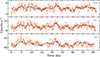 |
Fig. 1. EPIC light curves in the 0.2–12.0 keV energy range and OM light curve in B filter binned in 80 s intervals for clarity purposes. The black solid line represents the multi-fit sinusoidal function comprising three frequencies present in the X-ray light curves. |
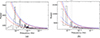 |
Fig. 2. Power spectra of J0826 obtained from (a) PN and (b) OM data. The red dashed and solid lines represent 95% single trial and global significance levels, respectively, while the blue dashed and solid lines represent 99% single trial and global significance levels, respectively. |
3.2. Folded light curves
We folded energy-resolved PN light curves (0.2–2.0 keV, 2.0–4.0 keV, 4.0–6.0, and 6.0–12.0 keV) at periods P1, P2, and P3 to check for the energy dependency (see, Figs. 3a–c). The reference time for folding was taken as MJD 58232, corresponding to the observation date of 2018-04-24 at 0 hr UT. The light curves were folded with a binning of 10 points in a phase. We also derived the fractional amplitude for P1, P2, and P3 by fitting a sinusoidal function to these light curves, in which the amplitude of the sinusoidal function denotes the derived value of fractional amplitudes. The derived values are given in Table 1, and are well within a 1σ level with each other. As can be seen from the folded light curves (Figs. 3a and c) and Table 1, no explicit energy dependency is present, which indicates that the photoelectric absorption in the accretion flow, which is typical in IPs, might not be playing a role for these variabilities. Inspection of the hardness ratio curves at periods P1 and P3 indeed does not show any variability. Moreover, the folded light curves at periods ∼1434 s and ∼922 s do not seem to show any significant variability.
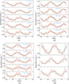 |
Fig. 3. Energy-dependent folded light curves of PN data at periods (a) P1, (b) P2, (c) P3, and (d) OM folded light curves at periods P1, P2, and P3. |
Energy-dependent fractional amplitude for periods P1, P2, and P3 obtained from the folded light curves.
The B-band light curve was also folded at the X-ray periods P1, P2, and P3 with a binning of 10 points in a phase, which are shown in Fig. 3d. The derived values of fractional amplitudes are 5.0 ± 0.8%, 3.1 ± 0.4%, and 2.9 ± 0.6% for P1, P2, and P3, respectively. The optical light curves are broadly consistent with the phasing of the X-ray light curves for periods P1 and P3 with maxima and minima of optical pulses centred on the X-ray maxima and minima, suggesting a common region where they are formed.
4. Spectral analysis
The background-subtracted X-ray spectra of J0826 were analysed in the energy range 0.3–10.0 keV using XSPEC version 12.12.0 (Arnaud 1996; Dorman & Arnaud 2001). Typically, the X-ray spectrum of IPs is characterised by the presence of multi-temperature thermal plasma emission components along with neutral total and partial covering absorbers. The continuum along with the H- and He-like ion emission lines of N, O, and Ne and strong iron emission line features at 6.4 keV (Fe Kα), 6.7 keV (Fe XXV), and 6.95 keV (Fe XXVI) are clearly seen in the spectra of J0826 (see Fig. 4). Therefore, to mimic the X-ray spectra of J0826, we used various model components in combination with each other available in XSPEC. The model tbabs was used to account for the X-ray absorption by the interstellar medium along the line of sight, sometimes in combination with convolution model partcov, which represents a partial covering absorber. The only parameter of partcov provides the value of the covering fraction (cf) of the absorber. To represent emission from collisionally ionised diffuse gas due to accretion, we used the model apec. It has three parameters: plasma temperature (T in keV), metal abundance relative to the solar value (Z), and normalisation (N in units of cm−5). The normalisation of the apec component is the volume emission measure and related by 
 , where D is the distance to the source,
  and
and  are the electron density and hydrogen density, respectively, and V is the emitting volume.
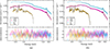 |
Fig. 4. MOS1, MOS2, PN, and RGS spectra of J0826 fitted simultaneously with (a) Model A and (b) Model B (see Sect. 4 for details). The bottom panel in each figure shows the χ2 contribution of data points for the respective model in terms of residual. |
We first used a simple model consisting of tbabs and adding from one to three apec components to represent the continuum plasma emission spectrum. The fit with three apec components was not able to account for emission line features of O, Ne, and N observed in the combined first order RGS spectrum. Therefore we added five Gaussian components at 0.43 keV, 0.50 keV, 0.57 keV, 0.65 keV, and 1.02 keV, which were identified as N VI, N VII, O VII, O VIII, and Ne X, respectively. The Gaussian component has three parameters: line energy (in keV), line width (σ), and line flux (F) in terms of photons cm−2 s−1, respectively. A further Gaussian component was used for the fluorescent iron line at 6.4 keV. However, this fit was poor with a χν2 value of ∼1.7. The partcov was then used along with tbabs due to the presence of residuals at low energies.
Thus, the model tbabs×(partcov×tbabs)×( +
+  ) slightly improved the fit with a χν2 value of 1.6. Further, adding a fourth apec component in this model remarkably improved the fit, with χν2 value of 1.30. We employed the ‘F-test’ to verify the necessity of the fourth apec component and found an F-statistic value of 40.6 with a null hypothesis probability of 5.4 × 10⁻²⁵. In this way, we defined our model A as ‘tbabs×(partcov×tbabs)×(
 +
+  )’. With model A, the metal abundance was found to be higher than solar with a value of 2.7 ± 0.2 (see Table A.1 for spectral parameters obtained from this fitting). Additionally, we investigated whether model A excluding Gaussian components could constrain the emission line features of various lines observed in the RGS spectrum. However, our analysis revealed that it was unable to do so.
Since we found a higher than solar value for the metal abundance with model A, we replaced apec with vapec to better understand the effect of individual abundances. The vapec model is the same as apec, but it allows for the modification of element abundances, such as He, C, N, O, Ne, Mg, Al, Si, S, Ar, Ca, Fe, and Ni. However, replacing apec with vapec and omitting Gaussian components in model A also resulted in the inadequate fitting of the emission line features. Therefore, we used a convolution model gsmooth with vapec, which broadens the emission lines. We fixed the power law index of gsmooth to 1 so that all of the lines are broadened by a constant velocity. In this manner, model B = ‘tbabs×(partcov×tbabs)×(gsmooth×  + gauss)’ was found to be the best-fit model with a χν2 value of 1.36, because it was able to represent various emission line features present in the spectra that the apec components could not represent. In model B, the N, O, Ne, Mg, Si, S, and Fe abundances were treated as free parameters. Meanwhile, the abundances of He, C, Al, Ar, Ca, and Ni were fixed to the solar values, as these elements do not contribute within the covered energy range, and therefore, their values could not be constrained when left free. In both models, we adopted abundances derived by Wilms et al. (2000). In order to further study the X-ray spectrum over a wider range, we also used the average spectrum from the BAT 105-month catalogue (Oh et al. 2018)4 along with the relevant response files5. We performed the combined spectral fitting in the 0.3–75.0 keV energy range using the best-fit model B (see Fig. 5). The unabsorbed bolometric flux in the 0.001–100.0 keV energy band was also calculated by incorporating the cflux component in models A and B. The spectral parameters derived from the simultaneous fitting to PN, MOS, RGS, and BAT spectra using model B together with the 90% confidence limit for a single parameter are given in Table 2.
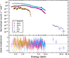 |
Fig. 5. MOS1, MOS2, PN, RGS, and BAT spectra of J0826 fitted simultaneously with Model B (see Sect. 4 for details). The bottom panel shows the χ2 contribution of data points for the respective model in terms of residual. |
Spectral parameters obtained from fitting the average spectra of J0826 using model B = ‘tbabs×(partcov×tbabs)×(gsmooth×  + gauss)’.
4.1. Phase-resolved spectroscopy
To explore the possible changes in the spectral parameters along the minimum and maximum phase ranges of P1 and P3, we extracted the MOS and PN spectra at pulse maximum and minimum identified on the total 0.2–12.0 keV light curve. The maximum and minimum phase ranges were identified as 0.7–1.3 and 0.3–0.7 for P1 and 0.6–1.1 and 0.1–0.6 for P3, respectively. The spectral fitting was performed using the best-fit model B and fixing all other parameters to the value found for the average spectrum except for the covering fraction, NH, cf, and normalisations of thermal and Gaussian components. The spectral parameters using the model B together with the 90% confidence limit for a single parameter are given in Tables 3 and 4. No substantial change in the parameters is found, for both periods; however, there are changes in the normalisation of the hotter vapec component N4. The value of N4 is larger at pulse maximum than at pulse minimum. On the other hand, these values are within 3–5σ consistent, which indicates that N4 shows a hint of variability at P1 and P3 periodicities. This might imply that the hotter component is the one that drives the variability at the two periods due to changes in the projected area.
Spectral parameters as derived from fitting the EPIC MOS and PN spectra at maximum and minimum phases of P1 using Model B.
Spectral parameters as derived from fitting the EPIC MOS and PN spectra at maximum and minimum phases of P3 using Model B.
4.2. Estimation of the WD mass
In order to derive an estimate of the WD mass, we used the post-shock region (PSR) model of Suleimanov et al. (2016, 2019), also known as ipolar in XSPEC. It has three parameters: fall height, WD mass, and normalisation. The fall height is the height from which the accretion flow starts to fall freely, that is, the magnetospheric radius (Rm). The aperiodic power spectrum shows no presence of break frequency; therefore, by making an assumption that Rm is equal to the co-rotation radius (Suleimanov et al. 2019; Shaw et al. 2020), we set the fall height parameter to be linked with the WD mass, as also done in Coughenour et al. (2022) and Tomsick et al. (2023). To avoid emission line effects, we fitted the spectra in the energy range 8.0–75.0 keV using the PSR model as ‘tbabs×(partcov×tbabs)×(atable{ipolar.fits})’, which resulted in a χν2 value of 0.75. The covering fraction and densities were set to the values found in the average spectral fitting. Hence, we derived the WD mass and normalisation to be 0.7 M⊙ and 7.0
 ×10−27, respectively. Moreover, the fall height was estimated to be 47.3 RWD (=36.5 × 10⁴ km), in which we have considered our candidate spin period value of ∼4588 s and the above-mentioned value of WD mass, along with the WD mass-radius relationship of Nauenberg (1972). We also derived the WD mass of 0.87
 by adopting the maximum temperature of
  keV found in the average spectral fitting as the shock temperature. The shock temperature (Ts) was related to WD mass as kTs =
  , where k is the Boltzmann constant, G is the gravitational constant, μ is the mean molecular weight, and mH is the mass of the hydrogen atom. The discrepancy with Parisi et al. (2012) is clearly due to the underestimated value of shock temperature derived using the lower quality data from Swift/XRT. Moreover, our derived value of the WD mass using two different methods is well within a 1σ consistent with each other and also in good agreement with the mean value found for CVs by Ramsay (2000) and (Pala et al. 2022).
5. Discussion
Our XMM-Newton observation of J0826 reveals the indications of magnetic accretion in this system, which are described in detail in the following sections.
5.1. The variability properties
The timing analyses revealed the presence of three X-ray peaks in the periodogram at P1 = 14103 ± 149 s, P2 = 5604 ± 34 s, and P3 = 4588 ± 25 s. These variabilities are found to be significant at the 95% global significance level. The same variability is also found in the optical data. The longer period at ∼3.92 h would naturally be ascribed to the orbital period of the system. However, we have a suspicion that P1 might be the half of the orbital period (PΩ), P3 the spin period (Pω), and P2 the beat between spin and orbital periods (Pω − Ω). The beat frequency (ω − Ω) arises in IPs due to the flipping of the accretion stream twice between the magnetic poles as the WD rotates with respect to the binary frame. If we consider P1 as the orbital period and P3 as the candidate spin period, then the estimated value of Pω − Ω comes out to be 6800 ± 65 s, which is beyond the 3σ significance level with the observed value of P2. Whereas, considering P1 as half of PΩ, the beat period is estimated to be 5479 ± 37 s. This value is well within a 2σ significance level with the observed value of P2, which represents our candidate beat period. Therefore, to reconcile the presence of the other two periodicities, if P3 represents the spin and  the orbital negative sideband (ω − Ω), the period P1 is half of the actual orbital period, which would be ∼7.84 h. A period this long would locate J0826 near the far end of the IP orbital period distribution (de Martino et al. 2020) and close to V2069 Cyg. The significance of these three peaks in the power spectra is high enough to consider them as true, suggesting an IP classification. If our candidate spin and beat periods are true periods, then J0826 accretes via a combination of disc and stream (disc-overflow accretion), with an equal fraction occurring via disc and stream, as evident from the equal values of fractional amplitudes obtained for Pω and Pω − Ω . J0826 would also have a degree of asynchronism Pω/PΩ of ∼0.16, comparatively larger than other IPs in the orbital period range of ∼7–8 h, such as V902 Mon (0.08), IGR J08390−4833 (0.05), Swift J0939.7−3224 (0.09), CXOGBS J174954.5−294335 (0.02), V2069 Cyg (0.03), and 1RXS J213344.1+510725 (0.02). Hence, J0826 would be located in the spin-orbit period plane among the slowest WD rotators for its orbital period.
Considering the candidate orbital period value of 7.84 h, the mean density of the secondary was estimated to be ∼1.7 g cm−3 (see Warner 1995, for formulae), which falls in the range of mean densities of a main-sequence star of G-K type (Allen 1976). Furthermore, we retrieved the optical spectrum by Parisi et al. (2012) 6 and found that the flux calibrated spectrum is quite off with respect to the optical photometry (about five times fainter), indicating either a non-optimal flux calibration or that the short (900 s) exposure caught the source at a lower flux, given its variability. We therefore normalised the spectrum to the continuum and identified a few weak absorption features ascribed to Ca I 4226 Å, weak 6122 Å, 6162 Å, Na I 5893 Å, Mg triplet (5167 Å, 5173 Å, and 5183 Å), and possibly the G-band at 4310 Å. The relatively low-resolution optical spectrum does not allow us to obtain a precise identification of the companion spectral type. Given the low-resolution spectrum, we only performed comparisons with stellar spectra from Jacoby et al. (1984), encompassing spectral types G9, K0, K4, and K5 (see, Fig. 6). A K6 star is not favoured due to the lack of strong molecular bands. The Ca I 6122 Å is very weak, indicating a spectral type not earlier than K3. Therefore, based on the limited information, we adopt a K4–K5 spectral type for the secondary. On the other hand, if the true orbital period is P1, the secondary star would be an M3.6 star (Knigge et al. 2011), and hence of a much later spectral type, to be consistent with the absorption features observed in the optical spectrum. These findings suggest that J0826 belongs to the category of long orbital period systems with evolved donors, which is consistent with the suggestions given by Beuermann et al. (1998), Baraffe & Kolb (2000), and Podsiadlowski et al. (2003). However, the identification of the true orbital period would reside in the study of radial velocities in the optical.
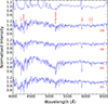 |
Fig. 6. Comparison of optical spectrum of Parisi et al. (2012) with stellar spectra of spectral type G9, K0, K4, and K5. |
Unlike the majority of IPs, the phase-folded analyses reveal that modulations at our proposed spin period and suspected half of the orbital period are energy independent, which suggests that these modulations are only due to the changes in the projected emitting area and not due to the photoelectric absorption in the accretion curtain. The 2Ω frequency, along with Ω frequency, was also seen in ∼62% of the sample studied by Parker et al. (2005) in the X-ray wavelength. Furthermore, optical modulations at our candidate half of the orbital period and spin period are in phase with the X-ray modulations, consistent with patterns seen in most IPs. This indicates that the optical spin pulsation originates in the magnetically confined accretion flow.
5.2. The post-shock region
The average X-ray spectral analyses reveal that the X-ray post-shock emitting region exhibits a multi-temperature structure with temperatures  keV,
keV,  keV,
keV,  keV, and
  keV. The spectrum indicates absorption by a total absorber with NH of ∼1.7 × 1020 cm−2 and a local absorber with NH of ∼1.6 × 1022 cm−2. The latter covers ∼27% of the X-ray source. The column density of the total absorber is much lower than the total interstellar value in the direction of the source, that is, 1.2 × 1021 cm−2 and consistent with the close distance of 366 pc derived from the Gaia parallax. The partial covering absorber density is lower than typical for IPs but still within the plausible range (Mukai 2017). The moderately weak equivalent width (EW) of the fluorescent iron line at 6.4 keV indicates that reflection from the WD surface does not play an important role in J0826, which also justifies the redundancy of this component in the spectral fits.
A lower limit to the accretion luminosity can be derived using the unabsorbed bolometric luminosity derived from the spectral fitting  1.7 × 1033 erg s−1, adopting the Gaia distance of 366 pc. However, to obtain a more reliable value of the accretion luminosity, we also considered the optical and near-IR (NIR) emission using the OM B-band and APASS B, V, g, r band measures, the 2MASS J, H, K and WISE W1, W2, W3, and W4 photometry7, corrected for interstellar extinction E(B − V)=0.02 estimated from the hydrogen column density found from X-ray spectral fit using the relation of Güver & Özel (2009). Here we note that J0826 when observed by XMM-Newton OM has been found at about the same level as in the APASS and consistently in the All-Sky Automated Survey for Supernovae (ASAS-SN; Shappee et al. 2014), which allows us to bridge the X-ray and ground-based photometry. Given the observed dereddened magnitudes of J0826 from B (15.1 mag) to NIR in the K-band (11.3 mag), only a donor with spectral type K2 or later located at 366 pc can account for the observed magnitudes. This indicates that the contribution of accretion at optical and NIR wavelengths is not dominant. Assuming a K4–K5 star, which is also evident from our earlier analysis (see Sect. 5.1), the excess of flux occurs in the optical and NIR bands (see Fig. 7), which comes out to be Fexcess ∼ 4.8−5.6 × 10⁻¹¹ erg cm−2 s−1, corresponding to a luminosity of L ∼ 7.7−9.0 × 1032 erg s−1. Therefore, we estimate an accretion luminosity as
  . Using Lacc = GMWD
 /RWD and adopting the WD mass value of 0.7 M⊙, we derive a mass accretion rate of 2.2−2.3 × 10⁻¹⁰ M⊙ yr−1. This value is at least two orders of magnitude lower than expected from magnetic braking (4.1 × 10⁻⁸ M⊙ yr−1; McDermott & Taam 1989) for an orbital period of ∼7.84 h. However, Baraffe & Kolb (2000) have shown that a low mass transfer rate (≤5 × 10⁻⁹ M⊙ yr−1) can be expected for orbital periods ≥6 h for evolved donors.
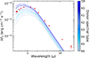 |
Fig. 7. Spectral energy distribution of J0826. The red filled circles represent the photometric data, while the dashed curves represent the donors of spectral type ranging from G9 to K6. |
The striking features of J0826 are substantial suprasolar abundance of N ( ), O (
 ), Ne (
 ), Mg (
 ), Si (
 ), S (
 ), and Fe (
 ). On the basis of anomalous UV line flux ratios obtained through UV spectroscopy, Gänsicke et al. (2003) estimated that at least 10–15% fraction of CVs may display large abundance anomalies. This might be attributed to the fact that these CVs may have gone through the thermal timescale mass transfer (TTMT) phase, in which the CV originally contained a donor more massive than the WD (Schenker et al. 2002; Podsiadlowski et al. 2003; Toloza et al. 2023). The suprasolar abundances with an indication of a long orbital period and evolved donor, collectively suggest that J0826 likely underwent TTMT (Schenker et al. 2004). Similar indications were also proposed for V1082 Sgr by Bernardini et al. (2013). Therefore, accurate photometry and polarimetry in optical wavelengths and UV spectroscopy will play an essential role in understanding the true nature and evolutionary status of this CV.
6. Conclusions
We have presented the first long X-ray observation of J0826 with XMM-Newton, which gives an indication of this CV belonging to the IP class. Here we summarise the main results:
-
The variability in X-rays and optical wavelengths shows modulations at short and long timescales. The long timescale variability (∼14 000 s) could be attributed to half of the true orbital period. Whereas ∼4600 s and ∼5600 s variabilities might correspond to spin and beat periods of the system, respectively. The simultaneous presence of spin and beat periods may suggest that J0826 accretes via disc-overflow.
-
The putative spin and orbital variabilities are energy independent, suggesting that these are due to the changes in the projected emitting area.
-
The post-shock region is comprised of a multi-temperature structure with a maximum temperature of about 43 keV, from which we derive a WD mass in the range of 0.82–0.93 M⊙, which is in good agreement with the WD mass of 0.7 ± 0.2 M⊙ derived using the PSR model.
-
The X-ray spectrum remarkably shows the presence of suprasolar abundances, which, together with the indication of a long orbital period and an evolved donor, collectively suggest that J0826 probably underwent a TTMT phase.
The zero-point value of 19.2661 for the B filter was used from the XMM-Newton Users Handbook available at https://xmm-tools.cosmos.esa.int/external/xmm_user_support/documentation/uhb/XMM_UHB.pdf
The spectrum is publicly available at CDS at http://cdsarc.u-strasbg.fr/viz-bin/qcat?J/A+A/545/A101.
The photometric measures are retrieved using VizieR access catalogue tool at CDS.
Acknowledgments
We thank the anonymous referee for providing valuable comments and suggestions that led to a significant improvement in the quality of the paper. This work is based on observations obtained with XMM-Newton, an ESA science mission with instruments and contributions directly funded by ESA Member States and NASA. We acknowledge the use of public data from the Swift data archive. This work has made use of the VizieR catalogue access tool, CDS, Strasbourg, France (DOI : 10.26093/cds/vizier) as well as of the European Space Agency (ESA) space mission Gaia data which are processed by the Gaia Data Processing and Analysis Consortium (DPAC). Funding for the DPAC is provided by national institutions, in particular, the institutions participating in the Gaia MultiLateral Agreement (MLA). The Gaia mission website is https://www.cosmos.esa.int/gaia. NR extends gratitude to Dr Arti Joshi and Mr Rahul Batra for helpful discussions. NM and DdM acknowledge financial support through ASI-INAF agreement 2017-14-H.0 (PI: T. Belloni).
References
- Aizu, K. 1973, Prog. Theor. Phys., 49, 1184 [CrossRef] [Google Scholar]
- Allen, C. W. 1976, Astrophysical Quantities [Google Scholar]
- Arnaud, K. A. 1996, ASP Conf. Ser., 101, 17 [Google Scholar]
- Bailer-Jones, C. A. L., Rybizki, J., Fouesneau, M., Demleitner, M., & Andrae, R. 2021, AJ, 161, 147 [Google Scholar]
- Baraffe, I., & Kolb, U. 2000, MNRAS, 318, 354 [NASA ADS] [CrossRef] [Google Scholar]
- Bernardini, F., de Martino, D., Mukai, K., et al. 2013, MNRAS, 435, 2822 [NASA ADS] [CrossRef] [Google Scholar]
- Beuermann, K., Baraffe, I., Kolb, U., & Weichhold, M. 1998, A&A, 339, 518 [NASA ADS] [Google Scholar]
- Coughenour, B. M., Tomsick, J. A., Shaw, A. W., et al. 2022, MNRAS, 511, 4582 [NASA ADS] [CrossRef] [Google Scholar]
- Cusumano, G., La Parola, V., Segreto, A., et al. 2010, A&A, 510, A48 [NASA ADS] [CrossRef] [EDP Sciences] [Google Scholar]
- de Martino, D., Bernardini, F., Mukai, K., Falanga, M., & Masetti, N. 2020, Adv. Space Res., 66, 1209 [Google Scholar]
- den Herder, J. W., Brinkman, A. C., Kahn, S. M., et al. 2001, A&A, 365, L7 [NASA ADS] [CrossRef] [EDP Sciences] [Google Scholar]
- Dorman, B., & Arnaud, K. A. 2001, ASP Conf. Ser., 238, 415 [NASA ADS] [Google Scholar]
- Gänsicke, B. T., Szkody, P., de Martino, D., et al. 2003, ApJ, 594, 443 [NASA ADS] [CrossRef] [Google Scholar]
- Güver, T., & Özel, F. 2009, MNRAS, 400, 2050 [Google Scholar]
- Hameury, J. M., King, A. R., & Lasota, J. P. 1986, MNRAS, 218, 695 [NASA ADS] [CrossRef] [Google Scholar]
- Hellier, C. 1995, ASP Conf. Ser., 85, 185 [NASA ADS] [Google Scholar]
- Jacoby, G. H., Hunter, D. A., & Christian, C. A. 1984, ApJS, 56, 257 [NASA ADS] [CrossRef] [Google Scholar]
- Jansen, F., Lumb, D., Altieri, B., et al. 2001, A&A, 365, L1 [NASA ADS] [CrossRef] [EDP Sciences] [Google Scholar]
- Knigge, C., Baraffe, I., & Patterson, J. 2011, ApJS, 194, 28 [Google Scholar]
- Lenz, P., & Breger, M. 2004, IAU Symp., 224, 786 [CrossRef] [Google Scholar]
- Mason, K. O., Breeveld, A., Much, R., et al. 2001, A&A, 365, L36 [NASA ADS] [CrossRef] [EDP Sciences] [Google Scholar]
- McDermott, P. N., & Taam, R. E. 1989, ApJ, 342, 1019 [NASA ADS] [CrossRef] [Google Scholar]
- Mukai, K. 2017, PASP, 129, 062001 [Google Scholar]
- Nauenberg, M. 1972, ApJ, 175, 417 [NASA ADS] [CrossRef] [Google Scholar]
- Oh, K., Koss, M., Markwardt, C. B., et al. 2018, ApJS, 235, 4 [Google Scholar]
- Pala, A. F., Gänsicke, B. T., Belloni, D., et al. 2022, MNRAS, 510, 6110 [NASA ADS] [CrossRef] [Google Scholar]
- Parisi, P., Masetti, N., Jiménez-Bailón, E., et al. 2012, A&A, 545, A101 [NASA ADS] [CrossRef] [EDP Sciences] [Google Scholar]
- Parker, T. L., Norton, A. J., & Mukai, K. 2005, A&A, 439, 213 [NASA ADS] [CrossRef] [EDP Sciences] [Google Scholar]
- Patterson, J. 1994, PASP, 106, 209 [Google Scholar]
- Podsiadlowski, P., Han, Z., & Rappaport, S. 2003, MNRAS, 340, 1214 [NASA ADS] [CrossRef] [Google Scholar]
- Ramsay, G. 2000, MNRAS, 314, 403 [NASA ADS] [CrossRef] [Google Scholar]
- Rosen, S. R., Mason, K. O., & Cordova, F. A. 1988, MNRAS, 231, 549 [NASA ADS] [CrossRef] [Google Scholar]
- Schenker, K., King, A. R., Kolb, U., Wynn, G. A., & Zhang, Z. 2002, MNRAS, 337, 1105 [NASA ADS] [CrossRef] [Google Scholar]
- Schenker, K., Wynn, G. A., & Speith, R. 2004, ASP Conf. Ser., 315, 8 [NASA ADS] [Google Scholar]
- Shappee, B. J., Prieto, J. L., Grupe, D., et al. 2014, ApJ, 788, 48 [Google Scholar]
- Shaw, A. W., Heinke, C. O., Mukai, K., et al. 2020, MNRAS, 498, 3457 [NASA ADS] [CrossRef] [Google Scholar]
- Strüder, L., Briel, U., Dennerl, K., et al. 2001, A&A, 365, L18 [Google Scholar]
- Suleimanov, V., Doroshenko, V., Ducci, L., Zhukov, G. V., & Werner, K. 2016, A&A, 591, A35 [NASA ADS] [CrossRef] [EDP Sciences] [Google Scholar]
- Suleimanov, V. F., Doroshenko, V., & Werner, K. 2019, MNRAS, 482, 3622 [NASA ADS] [CrossRef] [Google Scholar]
- Toloza, O., Gänsicke, B. T., Guzmán-Rincón, L. M., et al. 2023, MNRAS, 523, 305 [CrossRef] [Google Scholar]
- Tomsick, J. A., Kumar, S. G., Coughenour, B. M., et al. 2023, MNRAS, 523, 4520 [NASA ADS] [CrossRef] [Google Scholar]
- Turner, M. J. L., Abbey, A., Arnaud, M., et al. 2001, A&A, 365, L27 [CrossRef] [EDP Sciences] [Google Scholar]
- Vaughan, S. 2005, A&A, 431, 391 [NASA ADS] [CrossRef] [EDP Sciences] [Google Scholar]
- Warner, B. 1983, Astrophys. Space Sci. Libr., 101, 155 [CrossRef] [Google Scholar]
- Warner, B. 1995, Cataclysmic variable stars (Cambridge University Press), 28 [CrossRef] [Google Scholar]
- Wilms, J., Allen, A., & McCray, R. 2000, ApJ, 542, 914 [Google Scholar]
- Woelk, U., & Beuermann, K. 1996, A&A, 306, 232 [NASA ADS] [Google Scholar]
Appendix A: Spectral parameters obtained using model A
Spectral parameters obtained from fitting the average EPIC and RGS spectra of J0826 using model A= ‘tbabs×(partcov×tbabs)×( +
+  )’.
)’.
All Tables
Energy-dependent fractional amplitude for periods P1, P2, and P3 obtained from the folded light curves.
Spectral parameters obtained from fitting the average spectra of J0826 using model B = ‘tbabs×(partcov×tbabs)×(gsmooth× + gauss)’.
Spectral parameters as derived from fitting the EPIC MOS and PN spectra at maximum and minimum phases of P1 using Model B.
Spectral parameters as derived from fitting the EPIC MOS and PN spectra at maximum and minimum phases of P3 using Model B.
Spectral parameters obtained from fitting the average EPIC and RGS spectra of J0826 using model A= ‘tbabs×(partcov×tbabs)×( + )’.
All Figures
|
Fig. 1. EPIC light curves in the 0.2–12.0 keV energy range and OM light curve in B filter binned in 80 s intervals for clarity purposes. The black solid line represents the multi-fit sinusoidal function comprising three frequencies present in the X-ray light curves. |
| In the text | |
|
Fig. 2. Power spectra of J0826 obtained from (a) PN and (b) OM data. The red dashed and solid lines represent 95% single trial and global significance levels, respectively, while the blue dashed and solid lines represent 99% single trial and global significance levels, respectively. |
| In the text | |
|
Fig. 3. Energy-dependent folded light curves of PN data at periods (a) P1, (b) P2, (c) P3, and (d) OM folded light curves at periods P1, P2, and P3. |
| In the text | |
|
Fig. 4. MOS1, MOS2, PN, and RGS spectra of J0826 fitted simultaneously with (a) Model A and (b) Model B (see Sect. 4 for details). The bottom panel in each figure shows the χ2 contribution of data points for the respective model in terms of residual. |
| In the text | |
|
Fig. 5. MOS1, MOS2, PN, RGS, and BAT spectra of J0826 fitted simultaneously with Model B (see Sect. 4 for details). The bottom panel shows the χ2 contribution of data points for the respective model in terms of residual. |
| In the text | |
|
Fig. 6. Comparison of optical spectrum of Parisi et al. (2012) with stellar spectra of spectral type G9, K0, K4, and K5. |
| In the text | |
|
Fig. 7. Spectral energy distribution of J0826. The red filled circles represent the photometric data, while the dashed curves represent the donors of spectral type ranging from G9 to K6. |
| In the text | |
Current usage metrics show cumulative count of Article Views (full-text article views including HTML views, PDF and ePub downloads, according to the available data) and Abstracts Views on Vision4Press platform.
Data correspond to usage on the plateform after 2015. The current usage metrics is available 48-96 hours after online publication and is updated daily on week days.
Initial download of the metrics may take a while.