| Issue |
A&A
Volume 690, October 2024
|
|
|---|---|---|
| Article Number | L5 | |
| Number of page(s) | 8 | |
| Section | Letters to the Editor | |
| DOI | https://doi.org/10.1051/0004-6361/202451208 | |
| Published online | 07 October 2024 | |
Letter to the Editor
Probing the physics of star formation (ProPStar)
III. No evidence of dissipation of turbulence down to 20 mpc (4000 au) scale⋆
1
Max-Planck-Institut für extraterrestrische Physik, Giessenbachstrasse 1, D-85748 Garching, Germany
2
Istituto di Astrofisica e Planetologia Spaziali (IAPS), INAF, Via Fosso del Cavaliere 100, 00133 Roma, Italy
3
Department of Astronomy, The University of Texas at Austin, 2500 Speedway, Austin, TX 78712, USA
4
Center for Astrophysics | Harvard & Smithsonian, 60 Garden St, Cambridge, MA 02138, USA
5
Institut de Radioastronomie Millimétrique (IRAM), 300 rue de la Piscine, F-38406 Saint-Martin d’Hères, France
6
Department of Astronomy, University of Virginia, Charlottesville, VA 22904, USA
7
SKA Observatory, Jodrell Bank, Lower Withington, Macclesfield SK11 9FT, UK
8
IPAG, Université Grenoble Alpes, CNRS, F-38000 Grenoble, France
9
Green Bank Observatory, PO Box 2, Green Bank, WV 24944, USA
10
Department for Physics, Engineering Physics and Astrophysics, Queen’s University, Kingston, ON K7L 3N6, Canada
Received:
21
June
2024
Accepted:
26
August
2024
Abstract
Context. Turbulence is a key component of molecular cloud structure. It is usually described by a cascade of energy down to the dissipation scale. The power spectrum for subsonic incompressible turbulence is ∝k−5/3, while for supersonic turbulence it is ∝k−2.
Aims. We determine the power spectrum in an actively star-forming molecular cloud, from parsec scales down to the expected magnetohydrodynamic (MHD) wave cutoff (dissipation scale).
Methods. We analyzed observations of the nearby NGC 1333 star-forming region in three different tracers to cover the different scales from ∼10 pc down to 20 mpc. The largest scales are covered with the low-density gas tracer 13CO (1–0) obtained with a single dish, the intermediate scales are covered with single-dish observations of the C18O (3–2) line, while the smallest scales are covered in H13CO+ (1–0) and HNC (1–0) with a combination of NOEMA interferometer and IRAM 30m single-dish observations. The complementarity of these observations enables us to generate a combined power spectrum covering more than two orders of magnitude in spatial scale.
Results. We derive the power spectrum in an active star-forming region spanning more than 2 decades of spatial scales. The power spectrum of the intensity maps shows a single power-law behavior, with an exponent of 2.9 ± 0.1 and no evidence of dissipation. Moreover, there is evidence that the power spectrum of the ions to have more power at smaller scales than the neutrals, which is opposite to the theoretical expectations.
Conclusions. We show new possibilities for studying the dissipation of energy at small scales in star-forming regions provided by interferometric observations.
Key words: turbulence / stars: formation / ISM: clouds / ISM: molecules / ISM: individual objects: NGC 1333
Based on observations carried out under project number S21AD with the IRAM NOEMA Interferometer and 090-21 with the IRAM 30m telescope. IRAM is supported by INSU/CNRS (France), MPG (Germany) and IGN (Spain).
Corresponding author; This email address is being protected from spambots. You need JavaScript enabled to view it. .
NSF Astronomy and Astrophysics Postdoctoral Fellow.
© The Authors 2024
 Open Access article, published by EDP Sciences, under the terms of the Creative Commons Attribution License (https://creativecommons.org/licenses/by/4.0), which permits unrestricted use, distribution, and reproduction in any medium, provided the original work is properly cited.
This article is published in open access under the Subscribe-to-Open model.
Open access funding provided by Max Planck Society.
1. Introduction
Dense cores are the places where stars form (Pineda et al. 2023). These are the places with subsonic levels of turbulence (Goodman et al. 1998; Pineda et al. 2010; Friesen et al. 2017), and this transition to coherence has been discussed as possibly being linked to the dissipation of turbulence.
Turbulence in clouds has been typically studied using different tracers, which probe different scales of the cloud. For example, Larson (1981) found a correlation between linewidth and cloud size, σv ∝ L0.38. Further analysis using principal component analysis (PCA) showed that the velocity structure functions as a function of spatial scale, l, and is universal in molecular clouds (Heyer & Brunt 2004), δv ∝ l0.49; although further work showed some small variation (Heyer et al. 2009; Roman-Duval et al. 2011), the relation is approximately universal (see also references in McKee & Ostriker 2007; Heyer & Dame 2015).
In particular, the spatial power spectrum is used to study the lower density section of the cold neutral medium. Miville-Deschênes et al. (2010) measured the spatial power spectrum in the Polaris cloud using Herschel data, while Miville-Deschênes et al. (2016) showed a lack of evidence for the cutoff. These works focused on cirrus clouds, where gravity is not expected to play a major role.
In the case of star-forming molecular clouds, various works predict a turnover in the power spectrum at the dissipation scale (e.g., Elmegreen & Scalo 2004). Moreover, in the case of magnetohydrodynamic (MHD) turbulence, ions and neutrals at higher angular resolution are expected to display a difference in their linewidths at the same characteristic scale l (Li & Houde 2008). This is because there is a minimum MHD wave for wave propagation (λmin), below which MHD waves will not transmit, which would imply that ions should exhibit a turnover in the power spectrum at larger scales than neutrals.
In this study we present a comprehensive analysis of the power spectrum of spatial frequencies of gas in the NGC 1333 young cluster in the Perseus molecular cloud. We combine three data sets to study the power spectrum from parsec scales down to 20 mpc (4000 au).
2. Data
In order to properly probe the power spectrum over a wide spatial dynamical range we used three different data sets with different tracers. This enabled us to determine the power spectrum over an extended range of physical scales, which combined enabled us to cover more than two decades of physical scales. Figure 1 shows the integrated intensity maps used to analyze the scales covered, as well as the footprint of the higher angular resolution (and density tracer) observations used for the next spatial scale. The median spectra for the different data sets are presented in Appendix B and are shown in Fig. B.1.
For the largest scale, we used the 13CO (1–0) map of Perseus obtained with the FCRAO telescope by the COMPLETE survey (Ridge et al. 2006). This data has a resolution of 46″ and a noise level of 0.12 K.
The integrated intensity was calculated by adding the emission in the velocity range of −1 and 11.5 km s−1. The top left panel of Fig. 1 shows the integrated intensity map.
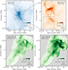 |
Fig. 1. Integrated intensity map of the different tracers used to observe the NGC1333 region. Top left: Large scale traced with 13CO (1–0). The footprint of the C18O (3–2) map is marked by the dashed box. Top right: Intermediate scale traced with C18O (3–2). The footprint of the interferometric data is marked by the dashed box. Bottom left and right: Highest angular resolution maps of H13CO+ and HNC (1–0), respectively. The beam size and scale bar are shown in the top right and bottom right corners, respectively. |
For intermediate scales, we used the C18O (3–2) observations of NGC 1333 taken with HARPS at JCMT (Curtis et al. 2010). The angular resolution of these observations is 17.7″ and it has a noise level of 0.18 K (Curtis et al. 2010).
The integrated intensity maps are calculated between 5.5 and 10 km s−1, which covers all the emission seen. The top right panel of Fig. 1 shows the integrated intensity map.
To trace small scales, we selected HNC and H13CO+ (1–0) because they are the brightest pair of molecular lines tracing the cloud, and have little contamination from outflows or shocks. They both cover a large fraction of the map and do not display resolved hyperfine components. The details on the image processing for these data are presented in Appendix A.
3. Analysis
3.1. Intensity power spectrum
The power spectrum of the integrated intensities is calculated using the Spatial Power Spectrum function, PS2, in +Turbstat+ (Koch et al. 2019) on the integrated intensity maps of the different transitions used (see Table A.1). We performed a beam correction on the power spectrum available on +Turbstat+, and in addition we only used spatial frequencies down to 3× the beam size, which allowed us to avoid the regime where the beam affects the power spectrum measurements. We also apodized the images with the +CosineBell+ kernel, which is available in +Turbstat+, to reduce the ringing effects due to the edge of the images1.
In the case of the interferometric observations, we padded the region not covered by the mosaic to reduce the effects from the map coverage on the power spectrum. The maps are filled with Gaussian noise outside the mosaic with a sigma level of the value listed in Table A.1. In this analysis we use spatial frequency, k = 1/λ, where λ is the spatial scale probed.
3.2. Stitching different scales and power-law fits
The individual PS2 from each molecular line has a different absolute amplitude, due to the difference in relative abundances and volumes traced by each molecular transition. However, the power-law exponent is inter-comparable. Therefore, we applied a normalisation coefficient to the PS2 derived for each map. We normalized the C18O power spectrum,  , to 1 at a spatial frequency of 10−0.5 pc−1, while the normalization parameter, fmol, is added to the spatial power spectrum, log PS2, mol + fmol, of each molecular transition as a free parameter, where mol is 13CO, H13CO+, and HNC, respectively. In practice, we generate two different data sets for analysis: D1 = {13CO, C18O, and H13CO+} and D2 = {13CO, C18O, and HNC}. We fit a single power law to each of the combined data sets as
 (1)
(1)
where k is the spatial frequency in units of pc−1, βi is the power spectrum power-law index, and Ai sets the amplitude of the relation fitted to the dataset Di. The power laws and all the normalization parameters are fitted simultaneously using EMCEE (Foreman-Mackey et al. 2013) (see Appendix C for details). The results are shown in Fig. 2, while the fitted parameters are listed in Table 1.
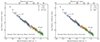 |
Fig. 2. Combined power spectrum of the three different datasets. The left and right panels respectively show the power spectrum with ion and neutrals at the smallest scales. The estimated MHD cutoff scale, 34 mpc, is marked by a vertical line. The fitted power law is shown by the dotted line, with exponents of β = 2.92 ± 0.11 and 2.94 ± 0.11 for the left and right panels, respectively. |
Results of the power-law fits.
4. Discussion
The physical interpretation of the intensity power spectrum relies on the assumption that the emission is optically thin, and therefore it is the power spectrum of the column density. Then the power spectrum is divided into three different regimes (e.g., Federrath et al. 2010). At large scales the transition between a plateau and a power law is associated with the injection scale of turbulence (usually expected to be similar to the cloud’s physical scale, McKee & Ostriker 2007). At intermediate scales, the power law is associated with the inertial range, which is the range of scales that characterize self-similarity in the flow. However, features at smaller scales could appear due to the influence of outflows or other feedback mechanisms (Nakamura & Li 2005; Padoan et al. 2009; Boyden et al. 2016; Xu et al. 2020). At small scales, the change in the slope of the power law is associated with the dissipation scale in the turbulence cascade. Our data appears to be beyond the range of the injection scales, but in what follows we discuss the other two features of the power spectra.
4.1. Exponent of the power spectra, β
We obtain a power spectrum with an average exponent of β = 2.9 ± 0.1, with the values of 2.92 ± 0.11 and 2.94 ± 0.11 for H13CO+ and HNC, respectively. This value is in agreement with the exponent found by Padoan et al. (2009) on the same region using 13CO (1–0) (see also Padoan et al. 2006), and it is also in rough agreement with the exponents found in H I, 12CO (1–0), 13CO (1–0), and dust extinction toward the Perseus molecular cloud (Pingel et al. 2018). However, Pingel et al. (2018) matches the pixel to the beam size and does not apply a beam correction in the power spectrum. This does not have an effect at large scales; however, it is important at scales closer to the beam and complicates a detailed comparison with the indexes obtained by Pingel et al. (2018). In other molecular clouds, studies with single-dish observations also recover an exponent comparable to the value determined here (Stutzki et al. 1998; Sun et al. 2006; Xu et al. 2020). Similar efforts focused on the power spectrum of the intensity taking advantage of interferometric mosaics combined with single-dish observations to recover all scales. In L1551, Swift & Welch (2008) found an exponent of 2.8±0.1 using C18O (1–0); while in different subregions of Orion A, Feddersen et al. (2019) found exponents between 3 and 4 using 12CO and 13CO (1–0), while slopes between 2.2 and 3.4 are determined in the case of C18O (1–0), see also Beuther et al. (2022) for analysis in a more distant high-mass region. In these cases, the most optically thin transition used is C18O (1–0), which still should become optically thick close to dense cores or embedded YSOs, and gives exponent values comparable to those found in this work. We note that the wide range of exponents reported in the literature complicates our comparison. This variation could suggest that the power-law exponent depends on the local environment, or it may indicate that large uncertainties in previous studies, possibly due to optical depth issues, are affecting the results.
Our derived slopes match those derived by Miville-Deschênes et al. (2016) from their combined spectrum ranging from scales between 0.01 and 50 pc (2.9 ± 0.1). However, the region considered in Miville-Deschênes et al. (2016) is a Galactic cirrus, with densities that are orders of magnitude lower than those characteristic of the gas in NGC 1333. Their 2.9 ± 0.1 exponent is comparable to that found in the infrared emission from cirrus observed with the Infrared Astronomical Satellite (IRAS) at 100 μm and Herschel at 250, 350, and 500 μm (Gautier et al. 1992; Miville-Deschênes et al. 2010). However, other Galactic cirrus clouds present different exponents in the power spectra derived from neutral atomic hydrogen (H I), with exponents between 2.59 and 3.7 on the largest scales (e.g., Pingel et al. 2013; Martin et al. 2015). Similarly, the power spectra of the dust thermal emission observed with Herschel toward the Large Magellanic cloud show exponents between 1.0 and 2.43 (Colman et al. 2022). This variability is found in multiple studies across tracers (Szotkowski et al. 2019; Koch et al. 2020), implying that the power-law exponent at large scales is not universal but is related to local physical conditions.
Numerical simulations of hydrodynamic (HD) and magnetohydrodynamic (MHD) turbulence are commonly used to link the power spectrum exponent to physical quantities, such as the sonic Mach number (ℳs), the Alfvén Mach number (ℳA), and the mixture between solenoidal and compressive turbulent modes (e.g., Federrath & Klessen 2013; Burkhart et al. 2015a). Kim & Ryu (2005) used numerical simulations of turbulence in a compressible and isothermal medium to show that trans-sonic turbulence (ℳs ≈ 1) produces power spectra with exponents around 1.73, close to the expected values from Kolmogorov turbulence, and shallower for increasing ℳs. A power spectrum slope of ≈3.0 corresponds to their results for ℳs ≈ 7.
Dedicated studies of MHD turbulence in self-gravitating giant molecular clouds show power spectrum exponents between 1.5 and 2.5 for simulations with 0.5 < ℳs < 20 and 0.7 < ℳA < 2.0 (Burkhart et al. 2015a). These slopes are hard to reconcile with our observational results and strongly suggest the effect of additional physics. Boyden et al. (2016) include the effect of stellar winds and magnetic fields in the MHD simulations aimed at reproducing the physical conditions in the Perseus molecular cloud and produce synthetic 12CO (1–0) emission observations. However, the slopes of their resulting power spectra are lower than in our results, falling in the range between 2.64 and 2.77. Boyden et al. (2018) showed that larger variations in temperature and abundance tend to flatten the power spectrum slope, and synthetic observations of MHD turbulence produced using full astrochemical networks yield slopes of ∼2.8.
Optical depth has a strong effect on the derived slope, such that the power spectrum slope of optically thick turbulent gas limits to 3.0 (Lazarian & Pogosyan 2004; Boyden et al. 2018). However, this is not the case in our observations, where the C18O and the higher-density tracers do not show evidence of being optically thick. Given the large degeneracy between the physical parameters that can result in our observed slope, we focus on other aspects of our observations, namely the similarity between the results for neutral and ionized species and the absence of a cut-off frequency in the power spectra.
Figures 2 and 3 show that there is a feature at log k≈0.9 pc−1 (≈150 mpc) there is a feature in the power spectra. However, this feature is not in the C18O power spectrum, which covers the same scales and with more independent samples. Therefore, this feature could be related to the shape of the interferometric mosaic since the 90″ scale (corresponding to log k ≈ 0.9 pc−1) is comparable to the width of the mosaic covering the southeast filamentary structure.
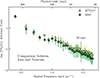 |
Fig. 3. Comparison of power spectra of ions and neutrals with our highest angular resolution data. The spectra are normalized as PS2(k) = 1 at the spatial frequency of 10 pc−1. The ions have a subtle but systematic excess of power at the smallest scales when compared to the neutrals. This is opposite to the expectations from ambipolar diffusion. |
4.2. Lack of difference between ions and neutrals
The neutral and ionized species are expected to decouple at certain scales due to ambipolar diffusion (Mestel & Spitzer 1956; Kulsrud & Pearce 1969; Mouschovias et al. 2011). This decoupling should introduce differences in the emission power spectra between neutral and ionized tracers (e.g., Houde et al. 2000).
The comparison of the complete power spectra between ions and neutrals (see Fig. 2) shows that they present the same power law and that neither has a turnover. This suggests that ions and neutrals do not present a substantial difference down to 20 mpc. Although both spectra agree well within 1σ, there is a systematic difference between the power spectra. Figure 3 shows this possible offset appears between the power spectra of HNC and H13CO+ for the highest angular resolution data. This is opposite to the prediction from ambipolar diffusion theories (e.g., Li & Houde 2008). Similarly, we cannot rule out that this discrepancy in the power spectra is related to systematic differences in the abundance and/or excitation conditions at higher angular scales (Gaches et al. 2015; Pineda et al. 2022; Tritsis et al. 2023).
4.3. MHD wave cutoff
In a molecular cloud, where the ionization level is low, Alfvén waves cannot propagate when the collision frequency between ions and neutrals is comparable to or smaller than the MHD wave frequency (Kulsrud & Pearce 1969; Mouschovias et al. 2011; Hennebelle & Lebreuilly 2023). Therefore, there is a critical length for wave propagation beyond which waves do not transmit. The critical length for wave propagation (Stahler & Palla 2005; Mouschovias et al. 2011) is obtained from
 (2)
(2)
where Bo is the unperturbed magnetic field and ⟨σ v⟩ is the rate coefficient for elastic collisions. The rate coefficient term is approximated by the Langevin term,
 (3)
(3)
for HCO+–H2 collisions (McDaniel & Mason 1973). We estimate the magnetic field strength, Bo, using the relation of Crutcher et al. (2010) (see also Myers & Basu 2021; Pattle et al. 2023), a typical volume density of 103.6 cm−3, and the median value of X(e) = 10−6.5 reported by Pineda et al. (2024). With these values, we obtain an MHD wave cutoff scale of 0.034 pc (7000 au). Therefore, we predict that if the turbulence is MHD in nature, then a dissipation scale should be observed at ≈0.034 pc (or ≈37″ at the distance of Perseus).
Previously, this scale had been proposed as a possible origin for the transition to coherence between the supersonic cloud and subsonic cores (∼0.1 pc; Goodman et al. 1998; Caselli et al. 2002; Pineda et al. 2010). Recent observations of dense gas with different tracers (e.g.,  and NH3) and angular resolutions show that the filaments present at the southern end of NGC 1333 present subsonic levels of turbulence at scales of ≈40″ (Friesen et al. 2017; Hacar et al. 2017; Dhabal et al. 2019; Sokolov et al. 2020), which corresponds to 0.034 pc or 7000 au at the distance of Perseus.
Finally, an improved estimate of the density or magnetic fields strength are needed to improve the obtained constraints. We used the volume density map of the region (Pineda et al. 2024) to determine a mean density 103.6 ± 0.2 cm−3, and with this uncertainty we derived an uncertainty on the MHD wave cutoff of ±13 mpc. This would push the λmin right below the scales sampled by these observations. Therefore, higher angular resolution and tighter constraints on the density and magnetic field strength in the region are required to make more progress in this topic.
4.4. Interpretation of single power-law spectrum
The combination of previous evidence for ions presenting a higher level of turbulence than neutrals at small scales suggests that a more exotic physical process is at play. Pineda et al. (2021) suggested that MHD waves could penetrate within dense cores and perturb the magnetic field lines. As a result, this process would inject kinetic energy into the ions at smaller scales, and therefore it could remove the scale for dissipation and possible differences between ions and neutrals.
Another possibility proposed by Hennebelle & Lebreuilly (2023) involves the effect of the dust grain inertia on the transfer of energy at smaller scales. This mechanism involves the interaction between dust particles and gas at small scales, which could inject energy in the denser regions remove the scale for dissipation.
On the other hand, different two-fluid simulations have studied the nature of the turbulence of both ions and neutrals (Oishi & Mac Low 2006; Burkhart et al. 2015b; Hu et al. 2024); however, these results show that the energy can be transported across the ambipolar diffusion (AD) scale. These results suggest that our understanding of the AD process in more realistic conditions is incomplete.
Unfortunately, all these possible explanations have not provided synthetic observations to better compare with the different observations, leaving the door open for improved comparisons. This includes possible effects due to radiative transfer and/or chemistry that must be taken into account to make the comparison.
5. Conclusions
We studied the molecular cloud structure across different densities and scales by combining three different data sets. We derived the combined power spectrum covering more than two orders of magnitude (from ≈3 pc to 20 mpc) in linear scale, with the smallest scales probed by two tracers: H13CO+ and HNC. The combined power spectrum fitting across all scales is well fit with a PS2(k)∝k−β function, where the exponents are 2.92 ± 0.11 and 2.94 ± 0.11 for H13CO+ and HNC, respectively. The power spectrum shows no evidence of a turnover (dissipation) down to 20 mpc.
The power spectra of the ions and neutrals are not substantially different. However, a systematic offset (extra) power is present in the ions at small scales when compared to the neutrals, which is opposite to the expectations of ambipolar diffusion models. These suggestive results, combined with the previous observations showing broader line widths for ions compared to neutrals (Pineda et al. 2021), imply that, contrary to the classical picture of turbulence dissipation, our understanding of AD processes is incomplete. More theoretical and observational work is needed (e.g., Hennebelle & Lebreuilly 2023; Hu et al. 2024) to explain these results and provide a general framework for the turbulence of ion and neutral, and to further confirm these differences.
Data availability
The code to reproduce the results of the paper are hosted at https://github.com/jpinedaf/NGC1333_NOEMA_turbulence
Acknowledgments
Part of this work was supported by the Max-Planck Society. We kindly thank the anonymous referee for the comments that helped improve the manuscript. EWK acknowledges support from the Smithsonian Institution as a Submillimeter Array (SMA) Fellow and the Natural Sciences and Engineering Research Council of Canada. DMS is supported by an NSF Astronomy and Astrophysics Postdoctoral Fellowship under award AST-2102405. JEP thanks M. A. Miville-Deschênes and F. Boulanger for stimulating discussion when starting the project, and P. Hennebelle, A. Traficante, and S. Molinari for valuable discussions. The authors acknowledge Interstellar Institute’s program With Two Eyes and the Core2disk-III residential program of Institut Pascal at Université Paris-Saclay, with the support of the program “Investissements d’Avenir” ANR-11-IDEX-0003-01. This work made use of Astropy (http://www.astropy.org): a community-developed core Python package and an ecosystem of tools and resources for astronomy (Astropy Collaboration 2013, 2018, 2022). This research has made use of NASA’s Astrophysics Data System Bibliographic Services.
References
- Astropy Collaboration (Robitaille, T. P., et al.) 2013, A&A, 558, A33 [NASA ADS] [CrossRef] [EDP Sciences] [Google Scholar]
- Astropy Collaboration (Price-Whelan, A. M., et al.) 2018, AJ, 156, 123 [Google Scholar]
- Astropy Collaboration (Price-Whelan, A. M., et al.) 2022, ApJ, 935, 167 [NASA ADS] [CrossRef] [Google Scholar]
- Beuther, H., Wyrowski, F., Menten, K. M., et al. 2022, A&A, 665, A63 [NASA ADS] [CrossRef] [EDP Sciences] [Google Scholar]
- Boyden, R. D., Koch, E. W., Rosolowsky, E. W., & Offner, S. S. R. 2016, ApJ, 833, 233 [NASA ADS] [CrossRef] [Google Scholar]
- Boyden, R. D., Offner, S. S. R., Koch, E. W., & Rosolowsky, E. W. 2018, ApJ, 860, 157 [NASA ADS] [CrossRef] [Google Scholar]
- Burkhart, B., Collins, D. C., & Lazarian, A. 2015a, ApJ, 808, 48 [NASA ADS] [CrossRef] [Google Scholar]
- Burkhart, B., Lazarian, A., Balsara, D., Meyer, C., & Cho, J. 2015b, ApJ, 805, 118 [NASA ADS] [CrossRef] [Google Scholar]
- Caselli, P., Benson, P. J., Myers, P. C., & Tafalla, M. 2002, ApJ, 572, 238 [Google Scholar]
- Colman, T., Robitaille, J.-F., Hennebelle, P., et al. 2022, MNRAS, 514, 3670 [NASA ADS] [CrossRef] [Google Scholar]
- Crutcher, R. M., Wandelt, B., Heiles, C., Falgarone, E., & Troland, T. H. 2010, ApJ, 725, 466 [NASA ADS] [CrossRef] [Google Scholar]
- Curtis, E. I., Richer, J. S., & Buckle, J. V. 2010, MNRAS, 401, 455 [NASA ADS] [CrossRef] [Google Scholar]
- Dhabal, A., Mundy, L. G., Chen, C.-Y., Teuben, P., & Storm, S. 2019, ApJ, 876, 108 [CrossRef] [Google Scholar]
- Elmegreen, B. G., & Scalo, J. 2004, ARA&A, 42, 211 [Google Scholar]
- Feddersen, J. R., Arce, H. G., Kong, S., Ossenkopf-Okada, V., & Carpenter, J. M. 2019, ApJ, 875, 162 [Google Scholar]
- Federrath, C., & Klessen, R. S. 2013, ApJ, 763, 51 [Google Scholar]
- Federrath, C., Roman-Duval, J., Klessen, R. S., Schmidt, W., & Mac Low, M. M. 2010, A&A, 512, A81 [NASA ADS] [CrossRef] [EDP Sciences] [Google Scholar]
- Foreman-Mackey, D., Hogg, D. W., Lang, D., & Goodman, J. 2013, PASP, 125, 306 [Google Scholar]
- Friesen, R. K., Pineda, J. E., Rosolowsky, E., et al. 2017, ApJ, 843, 63 [NASA ADS] [CrossRef] [Google Scholar]
- Gaches, B. A. L., Offner, S. S. R., Rosolowsky, E. W., & Bisbas, T. G. 2015, ApJ, 799, 235 [CrossRef] [Google Scholar]
- Gautier, T. N. I., Boulanger, F., Perault, M., & Puget, J. L. 1992, AJ, 103, 1313 [NASA ADS] [CrossRef] [Google Scholar]
- Goodman, A. A., Barranco, J. A., Wilner, D. J., & Heyer, M. H. 1998, ApJ, 504, 223 [Google Scholar]
- Hacar, A., Tafalla, M., & Alves, J. 2017, A&A, 606, A123 [NASA ADS] [CrossRef] [EDP Sciences] [Google Scholar]
- Hennebelle, P., & Lebreuilly, U. 2023, A&A, 674, A149 [NASA ADS] [CrossRef] [EDP Sciences] [Google Scholar]
- Heyer, M. H., & Brunt, C. M. 2004, ApJ, 615, L45 [NASA ADS] [CrossRef] [Google Scholar]
- Heyer, M., & Dame, T. M. 2015, ARA&A, 53, 583 [Google Scholar]
- Heyer, M., Krawczyk, C., Duval, J., & Jackson, J. M. 2009, ApJ, 699, 1092 [Google Scholar]
- Houde, M., Bastien, P., Peng, R., Phillips, T. G., & Yoshida, H. 2000, ApJ, 536, 857 [NASA ADS] [CrossRef] [Google Scholar]
- Hu, Y., Xu, S., Arzamasskiy, L., Stone, J. M., & Lazarian, A. 2024, MNRAS, 527, 3945 [Google Scholar]
- Kim, J., & Ryu, D. 2005, ApJ, 630, L45 [NASA ADS] [CrossRef] [Google Scholar]
- Koch, E. W., Rosolowsky, E. W., Boyden, R. D., et al. 2019, AJ, 158, 1 [NASA ADS] [CrossRef] [Google Scholar]
- Koch, E. W., Chiang, I.-D., Utomo, D., et al. 2020, MNRAS, 492, 2663 [NASA ADS] [CrossRef] [Google Scholar]
- Kulsrud, R., & Pearce, W. P. 1969, ApJ, 156, 445 [NASA ADS] [CrossRef] [Google Scholar]
- Larson, R. B. 1981, MNRAS, 194, 809 [Google Scholar]
- Lazarian, A., & Pogosyan, D. 2004, ApJ, 616, 943 [NASA ADS] [CrossRef] [Google Scholar]
- Li, H.-B., & Houde, M. 2008, ApJ, 677, 1151 [NASA ADS] [CrossRef] [Google Scholar]
- Martin, P. G., Blagrave, K. P. M., Lockman, F. J., et al. 2015, ApJ, 809, 153 [NASA ADS] [CrossRef] [Google Scholar]
- McDaniel, E. W., & Mason, E. A. 1973, The Mobility and Diffusion of Ions in Gases, Wiley Series in Plasma Physics (John Wiley& Sons) [Google Scholar]
- McKee, C. F., & Ostriker, E. C. 2007, ARA&A, 45, 565 [Google Scholar]
- Mestel, L., & Spitzer, Jr., L. 1956, MNRAS, 116, 503 [NASA ADS] [CrossRef] [Google Scholar]
- Miville-Deschênes, M. A., Martin, P. G., Abergel, A., et al. 2010, A&A, 518, L104 [NASA ADS] [CrossRef] [EDP Sciences] [Google Scholar]
- Miville-Deschênes, M. A., Duc, P. A., Marleau, F., et al. 2016, A&A, 593, A4 [Google Scholar]
- Mouschovias, T. C., Ciolek, G. E., & Morton, S. A. 2011, MNRAS, 415, 1751 [NASA ADS] [CrossRef] [Google Scholar]
- Myers, P. C., & Basu, S. 2021, ApJ, 917, 35 [NASA ADS] [CrossRef] [Google Scholar]
- Nakamura, F., & Li, Z.-Y. 2005, ApJ, 631, 411 [NASA ADS] [CrossRef] [Google Scholar]
- Oishi, J. S., & Mac Low, M.-M. 2006, ApJ, 638, 281 [NASA ADS] [CrossRef] [Google Scholar]
- Padoan, P., Juvela, M., Kritsuk, A., & Norman, M. L. 2006, ApJ, 653, L125 [NASA ADS] [CrossRef] [Google Scholar]
- Padoan, P., Juvela, M., Kritsuk, A., & Norman, M. L. 2009, ApJ, 707, L153 [NASA ADS] [CrossRef] [Google Scholar]
- Pattle, K., Fissel, L., Tahani, M., Liu, T., & Ntormousi, E. 2023, ASP Conf. Ser., 534, 193 [NASA ADS] [Google Scholar]
- Pineda, J. E., Goodman, A. A., Arce, H. G., et al. 2010, ApJ, 712, L116 [Google Scholar]
- Pineda, J. E., Schmiedeke, A., Caselli, P., et al. 2021, ApJ, 912, 7 [NASA ADS] [CrossRef] [Google Scholar]
- Pineda, J. E., Harju, J., Caselli, P., et al. 2022, AJ, 163, 294 [NASA ADS] [CrossRef] [Google Scholar]
- Pineda, J. E., Arzoumanian, D., Andre, P., et al. 2023, ASP Conf. Ser., 534, 233 [NASA ADS] [Google Scholar]
- Pineda, J. E., Sipilä, O., Segura-Cox, D. M., et al. 2024, A&A, 686, A162 [NASA ADS] [CrossRef] [EDP Sciences] [Google Scholar]
- Pingel, N. M., Stanimirović, S., Peek, J. E. G., et al. 2013, ApJ, 779, 36 [NASA ADS] [CrossRef] [Google Scholar]
- Pingel, N. M., Lee, M.-Y., Burkhart, B., & Stanimirović, S. 2018, ApJ, 856, 136 [CrossRef] [Google Scholar]
- Ridge, N. A., Di Francesco, J., Kirk, H., et al. 2006, AJ, 131, 2921 [Google Scholar]
- Roman-Duval, J., Federrath, C., Brunt, C., et al. 2011, ApJ, 740, 120 [NASA ADS] [CrossRef] [Google Scholar]
- Sokolov, V., Pineda, J. E., Buchner, J., & Caselli, P. 2020, ApJ, 892, L32 [NASA ADS] [CrossRef] [Google Scholar]
- Stahler, S. W., & Palla, F. 2005, The Formation of Stars (Wiley-VCH) [Google Scholar]
- Steer, D. G., Dewdney, P. E., & Ito, M. R. 1984, A&A, 137, 159 [NASA ADS] [Google Scholar]
- Stutzki, J., Bensch, F., Heithausen, A., Ossenkopf, V., & Zielinsky, M. 1998, A&A, 336, 697 [NASA ADS] [Google Scholar]
- Sun, K., Kramer, C., Ossenkopf, V., et al. 2006, A&A, 451, 539 [NASA ADS] [CrossRef] [EDP Sciences] [Google Scholar]
- Swift, J. J., & Welch, W. J. 2008, ApJS, 174, 202 [CrossRef] [Google Scholar]
- Szotkowski, S., Yoder, D., Stanimirović, S., et al. 2019, ApJ, 887, 111 [NASA ADS] [CrossRef] [Google Scholar]
- Tritsis, A., Basu, S., & Federrath, C. 2023, MNRAS, 521, 5087 [NASA ADS] [CrossRef] [Google Scholar]
- Virtanen, P., Gommers, R., Oliphant, T. E., et al. 2020, Nat. Methods, 17, 261 [Google Scholar]
- Xu, D., Offner, S. S. R., Gutermuth, R., & Oort, C. V. 2020, ApJ, 890, 64 [NASA ADS] [CrossRef] [Google Scholar]
Appendix A: Processing of IRAM data
The HNC (1–0) and H13CO+ (1–0) lines were observed with IRAM 30-m and NOrthern Extended Millimeter Array (NOEMA) and the details are described in Sec. A.1 and A.2, respectively. The combination procedure is described in Sec. A.3.
A.1. IRAM 30m telescope
The observations were carried out with the IRAM 30m telescope at Pico Veleta (Spain) on 2021 November 9, 10, and 11; and 2022 February 19, 20, under project 091-21. The EMIR E090 receiver and the FTS50 backend were employed. We used two spectral setups to cover the H13CO+ (1–0) and HNC (1–0) lines at 86.7 and 90.6 GHz (see Table A.1). We mapped a region of ≈150″×150″ with the On-the-Fly mapping technique, and using position switching. Data reduction was performed using the CLASS program of the GILDAS package2. The beam efficiency, Beff, is obtained using the Ruze formula (available in CLASS), and it is used to convert the observations into main beam temperatures, Tmb.
Spectral information for each of the spectral lines analyzed.
A.2. NOEMA interferometer
The observations were carried out with the IRAM NOEMA interferometer within the S21AD program using the Band 1 receiver. The observations were carried out on 2021 July 18, 19, and 21; August 10, 14, 15, 19, 22, and 29; and September 1 in the D configuration. We observed a total of 96 pointings, which were separated on four different scheduling blocks. The mosaic’s center is located at αJ2000 = 03h29m10.2s, δJ2000 = 31°13′49.4″. We use the PolyFix correlator with a LO frequency of 82.505 GHz and an instantaneous bandwidth of 31 GHz spread over two sidebands (upper and lower) and two polarisations. The centers of the two 7.744 GHz wide sidebands are separated by 15.488 GHz. Each sideband is composed of two adjacent basebands of ∼3.9 GHz width (inner and outer basebands). In total, there are thus eight basebands, which are fed into the correlator. The spectral resolution is 2 MHz throughout the 15.488 GHz effective bandwidth per polarization. Additionally, a total of 112 high-resolution chunks are placed, each with a width of 64 MHz and a fixed spectral resolution of 62.5 kHz. Both polarizations (H and V) are covered with the same spectral setup, and therefore the high-resolution chunks provide 66 dual polarisation spectral windows. The high spectral resolution windows used here are listed in Table A.1.
A.3. Image combination
The original IRAM 30m data is resampled to match the spectral setup of the NOEMA observations. We use the task +uvshort+ to generate the pseudo-visibilities from the 30-m data for each NOEMA pointing. The imaging is done with natural weighting, a support mask, and using the SDI deconvolution algorithm (Steer et al. 1984).
The noise level of the combined images is reported in Table A.1. The integrated intensity maps are calculated using the velocity ranges listed in Table A.1, this velocity range covers all the emission seen in both molecules. The bottom left and right panels of Fig. 1 show the integrated intensity maps for H13CO+ and HNC.
Appendix B: Median spectra
We show the median spectra for across the four different data cubes used in Fig. B.1. They are determined as the median value of all the values in the cubes.
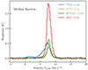 |
Fig. B.1. Typical spectra for the different tracers used calculated over the regions used in this work. |
Given the average spectra, we estimate the optical depth of the brightest line in the sample: HNC (1–0). We use the radiative transfer solution to estimate the optical depth as
 (B.1)
(B.1)
where Tp(HNC) is the observed line peak brightness, and Jν(T) is the brightness temperature of a black body with temperature T at frequency ν. For HNC (1–0) we assume the same excitation temperature of Tex = 12 K as used by Pineda et al. (2024), and obtain τ(HNC) = 0.23, which shows the emission is optically thin. We perform the same calculations with Tex = 10 K and obtain an optical depth of 0.31, confirming that the optically thin approximation is reasonable in this region.
Appendix C: Power-law fit with EMCEE
The +emcee+ fit is initialized starting from the result of the linear fit using the minimize function within the +scipy+ python package (Virtanen et al. 2020). In the +emcee+ run, we use uniform priors U(a, b), which is constant between a and b. We use U(1, 2.5) for  and AHNC, U(2.0, 3.4) for
  and βHNC, U(2, 3) for f13CO, U(−2, −1) for fH13CO+, and U(−1, 0.5) for fHNC, where the ranges are set to cover the best fit from the initial linear fit and without reaching the limits with the chains.
We used 56 random walkers, with 50 000 steps. We estimate an autocorrelation time of 80 steps, and therefore before analyzing, we discarded the first 600 steps and then thinned the samples by 40 to obtain better estimates. The corner plots for both fits are shown in Fig. C.1 and summarized in Table 1.
All Tables
All Figures
|
Fig. 1. Integrated intensity map of the different tracers used to observe the NGC1333 region. Top left: Large scale traced with 13CO (1–0). The footprint of the C18O (3–2) map is marked by the dashed box. Top right: Intermediate scale traced with C18O (3–2). The footprint of the interferometric data is marked by the dashed box. Bottom left and right: Highest angular resolution maps of H13CO+ and HNC (1–0), respectively. The beam size and scale bar are shown in the top right and bottom right corners, respectively. |
| In the text | |
|
Fig. 2. Combined power spectrum of the three different datasets. The left and right panels respectively show the power spectrum with ion and neutrals at the smallest scales. The estimated MHD cutoff scale, 34 mpc, is marked by a vertical line. The fitted power law is shown by the dotted line, with exponents of β = 2.92 ± 0.11 and 2.94 ± 0.11 for the left and right panels, respectively. |
| In the text | |
|
Fig. 3. Comparison of power spectra of ions and neutrals with our highest angular resolution data. The spectra are normalized as PS2(k) = 1 at the spatial frequency of 10 pc−1. The ions have a subtle but systematic excess of power at the smallest scales when compared to the neutrals. This is opposite to the expectations from ambipolar diffusion. |
| In the text | |
|
Fig. B.1. Typical spectra for the different tracers used calculated over the regions used in this work. |
| In the text | |
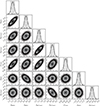 |
Fig. C.1. Corner plot for all parameters fitted. See Table 1 for a summary of the fits. |
| In the text | |
Current usage metrics show cumulative count of Article Views (full-text article views including HTML views, PDF and ePub downloads, according to the available data) and Abstracts Views on Vision4Press platform.
Data correspond to usage on the plateform after 2015. The current usage metrics is available 48-96 hours after online publication and is updated daily on week days.
Initial download of the metrics may take a while.