| Issue |
A&A
Volume 690, October 2024
|
|
|---|---|---|
| Article Number | A363 | |
| Number of page(s) | 6 | |
| Section | The Sun and the Heliosphere | |
| DOI | https://doi.org/10.1051/0004-6361/202451199 | |
| Published online | 22 October 2024 | |
A search for mode coupling in magnetic bright points
1
Department of Physics and Astronomy, California State University Northridge, Nordhoff St, Northridge, CA 91330, USA
2
Astrophysics Research Centre, School of Mathematics and Physics, Queen’s University, Belfast, BT7 1NN Northern Ireland, U.K.
Received:
20
June
2024
Accepted:
29
August
2024
Abstract
Context. Magnetic bright points (MBPs) are one of the smallest manifestations of the magnetic field in the solar atmosphere and are observed to extend from the photosphere up to the chromosphere. As such, they represent an excellent feature to use in searches for types of magnetohydrodynamic (MHD) waves and mode coupling in the solar atmosphere.
Aims. In this work, we aim to study wave propagation in the lower solar atmosphere by comparing intensity oscillations in the photosphere with the chromosphere via a search for possible mode coupling, in order to establish the importance of these types of waves in the solar atmosphere, and their contribution to heating the chromosphere.
Methods. These observations were conducted in July 2011 with the Rapid Oscillations of the Solar Atmosphere (ROSA) and the Hydrogen-Alpha Rapid Dynamics Camera (HARDCam) instruments at the Dunn Solar Telescope. Observations with good seeing were made in the G-band and Hα wave bands. Speckle reconstruction and several post facto techniques were applied to return science-ready images. The spatial sampling of the images was 0.069″/pixel (50 km/pixel). We used wavelet analysis to identify traveling MHD waves and derive frequencies in the different bandpasses. We isolated a large sample of MBPs using an automated tracking algorithm throughout our observations. Two dozen of the brightest MBPs were selected from the sample for further study.
Results. We find oscillations in the G-band MBPs, with frequencies between 1.5 and 3.6 mHz. Corresponding MBPs in the lower solar chromosphere observed in Hα show a frequency range of 1.4–4.3 mHz. In about 38% of the MBPs, the ratio of Hα to G-band frequencies was near two. Thus, these oscillations show a form of mode coupling where the transverse waves in the photosphere are converted into longitudinal waves in the chromosphere. The phases of the Hα and G-band light curves show strong positive and negative correlations only 21% and 12% of the time, respectively.
Conclusions. From simple estimates we find an energy flux of ≈45 × 103 W m−2 and show that the energy flowing through MBPs is enough to heat the chromosphere, although higher-resolution data are needed to explore this contribution further. Regardless, mode coupling is important in helping us understand the types of MHD waves in the lower solar atmosphere and the overall energy budget.
Key words: magnetohydrodynamics (MHD) / Sun: chromosphere / Sun: magnetic fields / Sun: oscillations / Sun: photosphere
Corresponding authors; This email address is being protected from spambots. You need JavaScript enabled to view it. , This email address is being protected from spambots. You need JavaScript enabled to view it. , This email address is being protected from spambots. You need JavaScript enabled to view it.
© The Authors 2024
 Open Access article, published by EDP Sciences, under the terms of the Creative Commons Attribution License (https://creativecommons.org/licenses/by/4.0), which permits unrestricted use, distribution, and reproduction in any medium, provided the original work is properly cited.
This article is published in open access under the Subscribe to Open model. This email address is being protected from spambots. You need JavaScript enabled to view it. to support open access publication.
1. Introduction
How the Sun transports energy through its dynamic lower solar atmosphere is a challenging topic that has been puzzling researchers for decades (e.g., see the recent reviews by Jess et al. 2015, 2023). Significant work in recent years has enabled magnetohydrodynamic (MHD) waves be not only detected in the Sun’s lower atmosphere but also studied in detail, notably with regard to their modal composition (Jess et al. 2017; Grant et al. 2022; Albidah et al. 2023), embedded energy flux (Bate et al. 2022; Molnar et al. 2023), rates of damping over both spatial and temporal domains (Grant et al. 2015; Gilchrist-Millar et al. 2021; Riedl et al. 2021), and the characteristics they demonstrate as they traverse solar plasma dominated by magnetic or plasma pressure (Khomenko & Cally 2019; Murabito et al. 2021; Kumar et al. 2024). Importantly, propagating MHD waves are believed to carry mechanical energy flux into the solar chromosphere, which they can subsequently dissipate to heat this layer of the atmosphere.
Of particular interest is what happens to embedded wave modes as they pass through regions of the solar atmosphere where the magnetic and plasma pressures are approximately equal, such as the so-called equipartition region (e.g., Cally & Goossens 2008; Grant et al. 2018; Houston et al. 2020). MHD wave mode conversion occurs in plasmas where the waves can change their modes as they propagate through mediums. Mode conversion is plausible when the MHD waves pass through regions characterized by density and magnetic field changes.
However, the promising wave heating models (i.e., those that can provide enough energy to heat the solar corona) often overlooked the potentially important role of heating the chromosphere and thus the need to understand energy transport in this region. The behavior of small magnetic structures called magnetic bright points (MBPs), is important in understanding the energy transport between the photosphere and lower chromosphere. MBPs are some of the smallest observable objects in the photosphere, appearing as intensity enhancements within the intergranular lanes, and have magnetic field strengths of over one kilogauss (Crockett et al. 2010). Although capable of carrying energy into the chromosphere, transverse MHD waves cannot easily dissipate their energy without first passing through an intermediary stage. However, compressible longitudinal modes can readily deposit their energy through shock formation in the solar atmosphere (Zhugzhda et al. 1995). Thus, transforming transverse wave modes into longitudinal modes can provide this heating mechanism (Kalkofen 1997). Transverse waves with frequency νk are converted into longitudinal waves at twice this frequency, νλ (2νk).
Evidence of this mode-coupling in network bright points (NBPs) has been presented (Bloomfield et al. 2004; McAteer et al. 2003). These longitudinal waves are predicted to shock and heat the chromosphere (Zhugzhda et al. 1995). Studies from McAteer et al. (2003) for mode coupling in the chromosphere were conducted with NBPs taken in the Ca II K3, Mg1b1, Mg1b2, and Hα bandpasses. Four NBPs were investigated and found to show possible transverse longitudinal wave propagation from the photosphere into the lower chromosphere. It was concluded that these bright points could produce energy transport in the chromosphere through mode coupling. We note that the McAteer study focused on NBPs found at chromospheric heights as brightenings (especially in Ca II K3) that are spatially coherent with small-scale magnetic elements, whereas here we focus on MBPs in the photosphere, that is, small-scale magnetic elements often found within intergranular lanes.
In this work, we searched for observational evidence of mode coupling by studying oscillations of MBPs observed in the photosphere (G-band) to the chromosphere (Hα). In Section 2, we present a summary of the Rapid Oscillations of the Solar Atmosphere (ROSA), the Hydrogen-Alpha Dynamics Camera (HARDCam) observations, and our data analysis. The results are then presented in Sect. 3 and discussed in comparison to previous studies in Sect. 4. We also investigate whether the phases of the observed oscillations are consistent with mode coupling and produce enough energy to heat the chromosphere. Finally, Sect. 5 summarizes our findings and future extensions of this work.
2. Observations and analysis
Observations of the decaying active region NOAA AR11249 (heliocentric coordinates S16.3, E03.3) were obtained with the ROSA (Jess et al. 2010) and HARDCam (Jess et al. 2012a) imaging instruments on 2011 July 11 using the Dunn Solar Telescope in Sacramento Peak, USA. Observations were conducted between 14:36 and 15:34 UT, with ROSA sampling the photosphere through a 9.20 Å (full width half maximum) G-band filter, while HARDCam obtained chromospheric observations through a 0.25 Å (full width half maximum) Hα filter. The ROSA and HARDCam observations employed  and
and  per pixel spatial samplings, respectively to obtain field of view sizes of
  and
and  . The exposure time for the G-band was 5 ms and was run at a cadence of 30.3 frames per second (fps). The narrowband Hα filter was run at a 27.9 fps cadence with a 35 ms exposure time. High-order adaptive optics (Rimmele 2004) were utilized to correct wavefront deformations in real time during these observations and the images were speckle-reconstructed using 32 → 1 and 35 → 1 restorations (Weigelt & Wirnitzer 1983; Wöger et al. 2008) for the G-band and Hα, respectively. The reconstructed ROSA images for this study are shown in Fig. 1 with the bright points used in the study labeled. We note that over the course of the 58-minute observation window, MBPs were detected within the boxes labeled 1–24. However, due to the image being a snapshot from a single point in time, it is possible that not all boxes simultaneously had MBPs present inside them. Furthermore, the MBPs have less contrast when observed in Hα, making them more difficult to visually identify in Fig. 1 (similar to the effects noted by Samanta et al. 2016).
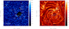 |
Fig. 1. From left to right: Reconstructed ROSA images for the G-band and Hα of active region NOAA AR11249. The overlying boxes show the corresponding MBPs. The dashed black line in the Hα images (just above the AR) indicates the region used for the time-distance plot shown in Fig. 4. |
We employed a MBP tracking algorithm (Crockett et al. 2010; Keys et al. 2020) to select MBPs from the G-band images. From the several hundred MBPs identified, we selected two dozen of the brightest MBPs, that is, with peak intensities over 2000 counts above the quiescent level for further temporal analysis. G-band MBPs were then matched to the co-aligned Hα images. We derived frequencies and periods for each co-spatial bandpass using the wavelet analysis techniques described by Jess et al. (2012a), first introduced by Torrence & Compo (1998). Then, light curves were extracted (Christian et al. 2019) for the G-band and Hα datasets for each MBP. Spatial regions of 40 × 40 and 20 × 20 pixels2 were chosen for the G-band and Hα, respectively. We note that the Hα images have a spatial sampling that is twice that of the G-band images, and hence 20 × 20 pixels2 in Hα occupies the same surface area as 40 × 40 pixels2 in the G-band, which helps keep the data processing consistent between the bandpasses. Most examples of MBPs show photospheric and chromospheric signatures that are approximately co-spatial. However, some small spatial offsets were identified in several MBPs, such as the MBP #11 near the edge of the detector, which may be a consequence of more heavily inclined magnetic field geometries in this location (e.g., Keys et al. 2013). Each light curve was then de-trended by a first-order polynomial to remove long-term variations in intensity and normalized to their subsequent mean. Wavelet and Fourier analysis was then performed on each MBP light curve. An example of the timing analysis is shown in Fig. 2.
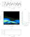 |
Fig. 2. Temporal analysis of a sample G-band light curve. (a) An MBP’s de-trended G-band light curve at 541, 411 (MBP #10; see Table 1). (b) Wavelet power transform along with locations at which detected power is at or above the 99% confidence level contained within the contours. (c) Summation of the wavelet power transform over time (full line) and the fast Fourier power spectrum (crosses) over time, plotted as a function of period. Both methods show strong detection near 540 seconds. (d) Global wavelet (solid line) and Fourier (dashed-dotted line) 99% significance levels. |
3. Results
Using our wavelet analysis techniques, we found strong periodic signals in the G-band and Hα time series for individual MBPs. The G-band periods range from ≈280–670 s, and the Hα periods range from 230–730 s, presented in Table 1. Table 1 gives the MBP number, the G-band position in (x, y) coordinates, the G-band and Hα frequencies and periods, the ratio of the Hα to G-band frequency, and the Pearson correlation coefficient. Our periods correspond to frequencies between 1.5 and 3.6 mHz in the photosphere (G-band) and frequencies of 1.4–4.3 mHz in the chromosphere (Hα). These G-band periods closely correspond to the well-known p-mode oscillation of 3–5 minutes (Lites et al. 1995). In the next section, we compare these results to mode coupling theory and examine whether these waves can contain enough energy to heat the chromosphere.
MBP frequencies and periods.
We compare the phases of the G-band and Hα folded light curves and sample folded light curves in Fig. 3. The G-band and Hα light curves were folded on their respective periods, and the cycle-to-cycle intensity variations were averaged to compute a total average phased light curve. We then computed the correlation of these light curves using the Pearson correlation coefficient (RP). These values are given in Table 1. Generally, the G-band and Hα folded light curves show weak correlations, with an average Pearson value of ≈0.04. However, several bright points, 1, 12, 16, 17, and 18 show moderate to strong positive correlations, and bright points 5, 7, and 10 show strong negative correlations. Additionally, 16 of the 24 MBPs show negative correlations. We compare these results to mode coupling theory in the Discussion.
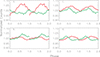 |
Fig. 3. Sample folded light curves comparing the G-band and Hα as a phase function, each light curve is folded on its respective periods. The MBPs for the G-band positions are shown as: a. 459, 632 (MBP #5); b. 670, 640 (MBP #13); c. 708, 846 (MBP #17); and d. 770, 642 (MBP #21). Signals for panel a show a strong anti-correlation. Signals from panel c show a strong correlation, while panels b and c show weaker positive correlations (see the main text). |
4. Discussion
4.1. Observed period and frequencies
Many previous studies have shown that the highest concentrations of power are found in highly magnetized regions, such as MPBs and intergranular lanes (Jess et al. 2023). Jess et al. (2007) identified 20 and 370 s periods in both the G-band and Hα blue wing, with a significant concentration of high-frequency activity (> 20 mHz) in the sunspot penumbra. We find the period for our G-band MBPs in the range 280–667 s (1.5–3.6 mHz). Stangalini et al. (2015) discovered kink waves amplified in the 2–8 mHz band, with a maximum of approximately 4.2 mHz in a study of 35 MBPs that used the photospheric Fe I doublet at 630 nm and the Ca II H core line at 396.9 nm to cover the chromosphere. This range of frequencies covers what we observed in the G-band and Hα. Although not in the G-band, Lites et al. (1993) found periods of 3–7 mHz in the photosphere. The Hα periods as we approach the chromosphere tend to be much lower, with McAteer et al. (2003) finding significant power down to 230 s (4.3 mHz). We find a range of periods for the MBPs in Hα (chromosphere) of 235–726 s (1.4–4.3 mHz). Morton et al. (2012) identified longitudinal (sausage) modes in Hα with periods of 197 s. Our typical Hα period is 435 s, or 2.3 mHz, with the lowest periods being about 235 s (4.3 mHz), which is consistent with the McAteer value.
4.2. Comparison to mode coupling theory
Theory has shown that transverse (kink) waves created in the photosphere can be converted into longitudinal waves at twice the frequency. Ulmschneider et al. (1991) found that monochromatic transverse waves of period Pk transferred energy mainly to longitudinal waves of half the period, Pl = Pk/2, but also transferred some energy, although much less, to waves with the period Pl = Pk. Several observational studies have found supporting evidence for this mode coupling. McAteer et al. (2003) found longitudinal waves (with frequencies between 2.6 and 3.8 mHz) in the chromosphere and transverse (kink) waves in the photosphere (with frequencies between 1.3 and 1.9 mHz). This was clear evidence of mode coupling with the longitudinal wave at twice the frequency of the transverse wave. Additional studies by Morton et al. (2012) found coupling of kink and sausage waves in the chromosphere. These waves were out of phase, possibly showing nonlinear resonance conditions. In a study of Type I spicules, Jess et al. (2012b) found a form of “reverse” mode coupling where transverse oscillations found in the chromosphere with Hα (periods of 65–220 s) were linked to longitudinal waves in the photosphere (periods of 130–440 s). Here, we find G-band frequencies ranging from 1.5–3.6 mHz and Hα frequencies ranging from 1.4–4.3 mHz. Our range of Hα frequencies covers the range found by McAteer et al. (2003), and we find that 9 of 24 MBPs (38%) have ratios of Hα to G-band frequencies greater than 1.5, consistent with predictions of mode coupling. An additional 12 of the 24 MBPs had ratios closer to 1, consistent with the lesser mode (Ulmschneider et al. 1991). We determined the wave types based on the ratios of Hα to G-band frequencies observed in simple mode coupling theory. We do not observe strong wave patterns (such as that seen in Jess et al. 2012b, in time-distance plots) as is evident in our time-distance plot in Fig. 4, nor do we have velocity information. Thus, we have little information for determining the wave nature. Future studies will have to wait for higher spatial resolution observations, such as those available with the Daniel K. Inouye Solar Telescope (DKIST).
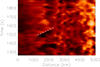 |
Fig. 4. Time-distance plot for Hα with the motion of a bright filament indicated by the dashed white line and moving at approximately 12.6 km/s. The extraction region from above the sunspot is indicated in the Hα image in Fig. 1b (see the main text). |
4.3. Phases
Simple mode coupling theory (Kalkofen 1997) suggests the transverse (kink) waves formed in the photosphere are in phase with the longitudinal (sausage) waves in the chromosphere. Lites et al. (1995) found strong phase coherence for frequencies near 5 mHz between these two waves, with all phase coherence disappearing at the highest frequencies. We find more than half of our MBPs (13/24) show in-phase oscillations between the G-band (photosphere) and Hα (chromosphere) with transverse and longitudinal wave types, respectively. However, phases of the Hα and G-band light curves show strong positive and negative correlations only 21% and 12% of the time, respectively. Most of these in-phase MBPs have ratios of Hα to G-band frequencies greater than 1, supporting simple mode coupling theory. The other MBPs are out of phase and generally have frequency ratios of less than 1. Only four MBPs show strong positive correlations when comparing the phases of the G-band and Hα folded light curves. This lack of strong correlations may be a function of poor matching from the G-band to Hα bands, as features in the Hα are more difficult to trace.
4.4. Energy budget
One of the important aspects of detecting mode coupling between the photosphere and chromosphere is determining whether the longitudinal waves produce sufficient energy to heat the outer solar atmosphere. Jess et al. (2009) provided the first observational evidence of the torsional (Alfvén) waves, detected as full width half maximum oscillations in a small MBP through the lower solar atmosphere (with periods on the order of 126–700 s). They estimated an energy flux of ≈15 000 W m−2 carried by these waves. Similar to our study, ROSA observations of MHD waves by Morton et al. (2012) found sufficient energy to heat the corona with an estimated energy flux for the incompressible fast kink mode of 4300 ± 2700 W m−2 and an estimated wave energy flux for the compressible fast MHD sausage mode of 11 700 ± 3800 W m−2. Jess et al. (2009) estimated the energy flux for an Alfvén wave as:
 (1)
(1)
Where ρ is the mass density, and vp and vA are the phase and Alfvén velocities, respectively. It is extremely difficult to estimate or infer all three of these plasma quantities simultaneously to a high degree of precision, and our energy flux estimate is an approximation. The density is normally taken from analytical models, such as the 1.3 × 10⁻⁸ kg m−3 used in Jess et al. (2012b), although modern inversion routines may be better able to estimate this quantity using full Stokes polarimetry (e.g., Hazel Asensio Ramos et al. 2008; STIC de la Cruz Rodríguez et al. 2019; NICOLE Socas-Navarro et al. 2019; and DeSIRe Ruiz Cobo et al. 2022). Similarly, the Alfvén velocity requires an understanding of the torsional velocity amplitudes of the embedded wave, which is only possible through spectroscopic means (e.g., the 22 km/s estimated by Jess et al. 2009). Typically, the phase velocity of the wave is a more straightforward property to estimate, since it can be linked to either the phase lag between signatures seen at different heights of the solar atmosphere (e.g., Jess et al. 2012c) or the physical tracking of wave motion captured using time-distance seismology (e.g., Morton et al. 2012; Krishna Prasad et al. 2019). In our present work, Fig. 4 shows a time-distance diagram highlighting dynamical motion with velocities on the order of 12.6 km/s. In reality, the true velocity may be higher than 12.6 km/s due to inclination effects with respect to the observer’s line of sight, although this still provides a lower estimate of the chromospheric dynamical velocities associated with MBPs. We note that models for flux tubes emerging through the photosphere show their horizontal velocity growing rapidly with height (Ulmschneider et al. 1991). Thus, we expect there to be some horizontal component to the flux tube for heating as it reaches the chromosphere. Using this measured velocity (Fig. 4), alongside the density and Alfvén velocity values of ρ = 1.3 × 10⁻⁸ kg m−3 and vA = 22 km/s, respectively, we calculated an energy flux of ≈45 × 103 W m−2. We note that this energy flux is sufficient to heat localized areas of the chromosphere and agrees with the energy estimates put forward by Erdélyi & Fedun (2007).
Yadav et al. (2021) also found that longitudinal waves supply enough energy to heat the chromosphere in the solar plage. Thus, based on our work, the idea of mode coupling remains as a process for heating the solar chromosphere and corona remains viable. Future studies that include velocity information, such as those available with the new DKIST instruments, can further our understanding of the coronal heating issue.
5. Conclusion
We have used high temporal and spatial resolution observations of the solar photosphere and chromosphere to search for mode coupling in the solar atmosphere. Two dozen MBPs were studied and found to have frequencies between 1.5 and 3.6 mHz in the photosphere (G-band) and frequencies of 1.4–4.3 mHz in the chromosphere (Hα). About 38% of the MBPs show the expected frequency doubling for transverse waves in the photosphere converted into longitudinal waves in the chromosphere. More than half of our MBPs (13/24) show in-phase oscillations between the G-band (photosphere) and Hα (chromosphere) with transverse and longitudinal wave types, respectively. We find an energy flux of ≈45 × 103 W m−2, in agreement with previous studies which show that this mode coupling produces high enough energy fluxes to heat the solar chromosphere. Future high temporal and spatial resolution studies that include velocity information, such as those available with the new DKIST instruments are needed to further our understanding of wave propagation and heating in the solar atmosphere.
Acknowledgments
We thank the CSUN Department of Physics and Astronomy for supporting this project. We acknowledge partial support of this project from NASA grants 19-HSODS-0004 and 21-SMDSS21-0047. We thank D. Gilliam and the Dunn Solar Telescope staff for their excellent support of the observations for this project. We wish to acknowledge scientific discussions with the Waves in the Lower Solar Atmosphere (WaLSA; http://www.WaLSA.team/) team, which has been supported by the Research Council of Norway (project no. 262622), The Royal Society (award no. Hooke18b/SCTM; Jess et al. 2021), and the International Space Science Institute (ISSI Team 502). D.B.J. acknowledges support from the Leverhulme Trust via the Research Project Grant RPG-2019-371. D.B.J. wishes to thank the UK Science and Technology Facilities Council (STFC) for the consolidated grants ST/T00021X/1 and ST/X000923/1. D.B.J. and P.H.K. also acknowledge funding from the UK Space Agency via the National Space Technology Programme (grant SSc-009). We thank an anonymous referee for comments improving the manuscript.
References
- Albidah, A. B., Fedun, V., Aldhafeeri, A. A., et al. 2023, ApJ, 954, 30 [NASA ADS] [CrossRef] [Google Scholar]
- Asensio Ramos, A., Trujillo Bueno, J., & Landi DeglInnocenti, E. 2008, ApJ, 683, 542 [NASA ADS] [CrossRef] [Google Scholar]
- Bate, W., Jess, D. B., Nakariakov, V. M., et al. 2022, ApJ, 930, 129 [NASA ADS] [CrossRef] [Google Scholar]
- Bloomfield, D. S., McAteer, R. J., Lites, B. W., et al. 2004, ApJ, 617, 623 [NASA ADS] [CrossRef] [Google Scholar]
- Cally, P. S., & Goossens, M. 2008, Sol. Phys., 251, 251 [Google Scholar]
- Christian, D., Kuridze, D., Jess, D., Yousefi, M., & Mathioudakis, M. 2019, Res. Astron. Astrophys., 19, 101 [CrossRef] [Google Scholar]
- Crockett, P., Mathioudakis, M., Jess, D., et al. 2010, ApJ, 722, L188 [NASA ADS] [CrossRef] [Google Scholar]
- de la Cruz Rodríguez, J., Leenaarts, J., Danilovic, S., & Uitenbroek, H. 2019, A&A, 623, 74 [Google Scholar]
- Erdélyi, R., & Fedun, V. 2007, Science, 318, 1572 [CrossRef] [Google Scholar]
- Gilchrist-Millar, C. A., Jess, D. B., Grant, S. D. T., et al. 2021, Philos. Trans. R. Soc. Lond. Ser. A, 379, 20200172 [NASA ADS] [Google Scholar]
- Grant, S. D. T., Jess, D. B., Moreels, M. G., et al. 2015, ApJ, 806, 132 [Google Scholar]
- Grant, S. D. T., Jess, D. B., Zaqarashvili, T. V., et al. 2018, Nat. Phys., 14, 480 [Google Scholar]
- Grant, S. D. T., Jess, D. B., Stangalini, M., et al. 2022, ApJ, 938, 143 [NASA ADS] [CrossRef] [Google Scholar]
- Houston, S. J., Jess, D. B., Keppens, R., et al. 2020, ApJ, 892, 49 [NASA ADS] [CrossRef] [Google Scholar]
- Jess, D., Andić, A., Mathioudakis, M., Bloomfield, D., & Keenan, F. 2007, A&A, 473, 943 [NASA ADS] [CrossRef] [EDP Sciences] [Google Scholar]
- Jess, D. B., Mathioudakis, M., Erdélyi, R., et al. 2009, Science, 323, 1582 [Google Scholar]
- Jess, D. B., Mathioudakis, M., Christian, D. J., et al. 2010, Sol. Phys., 261, 363 [NASA ADS] [CrossRef] [Google Scholar]
- Jess, D. B., De Moortel, I., Mathioudakis, M., et al. 2012a, ApJ, 757, 160 [NASA ADS] [CrossRef] [Google Scholar]
- Jess, D. B., Pascoe, D. J., Christian, D. J., et al. 2012b, ApJ, 744, L5 [NASA ADS] [CrossRef] [Google Scholar]
- Jess, D. B., Shelyag, S., Mathioudakis, M., et al. 2012c, ApJ, 746, 183 [Google Scholar]
- Jess, D. B., Morton, R. J., Verth, G., et al. 2015, Space Sci. Rev., 190, 103 [Google Scholar]
- Jess, D. B., Van Doorsselaere, T., Verth, G., et al. 2017, ApJ, 842, 59 [Google Scholar]
- Jess, D. B., Keys, P. H., Stangalini, M., & Jafarzadeh, S. 2021, Philos. Trans. R. Soc. Lond. Ser. A, 379, 20200169 [NASA ADS] [Google Scholar]
- Jess, D. B., Jafarzadeh, S., Keys, P. H., et al. 2023, Liv. Rev. Sol. Phys., 20, 1 [NASA ADS] [CrossRef] [Google Scholar]
- Kalkofen, W. 1997, ApJ, 486, L145 [NASA ADS] [CrossRef] [Google Scholar]
- Keys, P. H., Mathioudakis, M., Jess, D. B., et al. 2013, MNRAS, 428, 3220 [NASA ADS] [CrossRef] [Google Scholar]
- Keys, P., Reid, A., Mathioudakis, M., et al. 2020, A&A, 633, A60 [NASA ADS] [CrossRef] [EDP Sciences] [Google Scholar]
- Khomenko, E., & Cally, P. S. 2019, ApJ, 883, 179 [Google Scholar]
- Krishna Prasad, S., Jess, D., & Van Doorsselaere, T. 2019, Front. Astron. Space Sci., 6, 57 [NASA ADS] [CrossRef] [Google Scholar]
- Kumar, P., Nakariakov, V. M., Karpen, J. T., & Cho, K.-S. 2024, Nat. Commun., 15, 2667 [NASA ADS] [CrossRef] [Google Scholar]
- Lites, B., Rutten, R., & Kalkofen, W. 1993, ApJ, 414, 345 [NASA ADS] [CrossRef] [Google Scholar]
- Lites, B., Low, B., Martinez Pillet, V., et al. 1995, ApJ, 446, 877 [NASA ADS] [CrossRef] [Google Scholar]
- McAteer, R. J., Gallagher, P. T., Williams, D. R., et al. 2003, ApJ, 587, 806 [NASA ADS] [CrossRef] [Google Scholar]
- Molnar, M. E., Reardon, K. P., Cranmer, S. R., Kowalski, A. F., & Milić, I. 2023, ApJ, 945, 154 [NASA ADS] [CrossRef] [Google Scholar]
- Morton, R. J., Verth, G., Jess, D. B., et al. 2012, Nat. Commun., 3, 1315 [Google Scholar]
- Murabito, M., Stangalini, M., Baker, D., et al. 2021, A&A, 656, A87 [NASA ADS] [CrossRef] [EDP Sciences] [Google Scholar]
- Riedl, J. M., Gilchrist-Millar, C. A., Van Doorsselaere, T., Jess, D. B., & Grant, S. D. T. 2021, A&A, 648, A77 [NASA ADS] [CrossRef] [EDP Sciences] [Google Scholar]
- Rimmele, T. R. 2004, ApJ, 604, 906 [NASA ADS] [CrossRef] [Google Scholar]
- Ruiz Cobo, B., Quintero Noda, C., Gafeira, R., et al. 2022, A&A, 660, 37 [Google Scholar]
- Samanta, T., Henriques, V., Banerjee, D., et al. 2016, ApJ, 828, 23 [NASA ADS] [CrossRef] [Google Scholar]
- Socas-Navarro, H., de la Cruz Rodríguez, J., Asensio Ramos, A., Trujillo Bueno, J., & Ruiz Cobo, B. 2019, A&A, 577, 7 [Google Scholar]
- Stangalini, M., Giannattasio, F., & Jafarzadeh, S. 2015, A&A, 577, A17 [NASA ADS] [CrossRef] [EDP Sciences] [Google Scholar]
- Torrence, C., & Compo, G. P. 1998, BAMS, 79, 61 [NASA ADS] [CrossRef] [Google Scholar]
- Ulmschneider, P., Zähringer, K., & Musielak, Z. 1991, A&A, 241, 625 [NASA ADS] [Google Scholar]
- Weigelt, G., & Wirnitzer, B. 1983, Opt. Lett., 8, 389 [NASA ADS] [CrossRef] [Google Scholar]
- Wöger, F., Von der Lühe, O., & Reardon, K. 2008, A&A, 488, 375 [NASA ADS] [CrossRef] [EDP Sciences] [Google Scholar]
- Yadav, N., Cameron, R. H., & Solanki, S. K. 2021, A&A, 652, A43 [NASA ADS] [CrossRef] [EDP Sciences] [Google Scholar]
- Zhugzhda, Y. D., Bromm, V., & Ulmschneider, P. 1995, A&A, 300, 302 [NASA ADS] [Google Scholar]
All Tables
All Figures
|
Fig. 1. From left to right: Reconstructed ROSA images for the G-band and Hα of active region NOAA AR11249. The overlying boxes show the corresponding MBPs. The dashed black line in the Hα images (just above the AR) indicates the region used for the time-distance plot shown in Fig. 4. |
| In the text | |
|
Fig. 2. Temporal analysis of a sample G-band light curve. (a) An MBP’s de-trended G-band light curve at 541, 411 (MBP #10; see Table 1). (b) Wavelet power transform along with locations at which detected power is at or above the 99% confidence level contained within the contours. (c) Summation of the wavelet power transform over time (full line) and the fast Fourier power spectrum (crosses) over time, plotted as a function of period. Both methods show strong detection near 540 seconds. (d) Global wavelet (solid line) and Fourier (dashed-dotted line) 99% significance levels. |
| In the text | |
|
Fig. 3. Sample folded light curves comparing the G-band and Hα as a phase function, each light curve is folded on its respective periods. The MBPs for the G-band positions are shown as: a. 459, 632 (MBP #5); b. 670, 640 (MBP #13); c. 708, 846 (MBP #17); and d. 770, 642 (MBP #21). Signals for panel a show a strong anti-correlation. Signals from panel c show a strong correlation, while panels b and c show weaker positive correlations (see the main text). |
| In the text | |
|
Fig. 4. Time-distance plot for Hα with the motion of a bright filament indicated by the dashed white line and moving at approximately 12.6 km/s. The extraction region from above the sunspot is indicated in the Hα image in Fig. 1b (see the main text). |
| In the text | |
Current usage metrics show cumulative count of Article Views (full-text article views including HTML views, PDF and ePub downloads, according to the available data) and Abstracts Views on Vision4Press platform.
Data correspond to usage on the plateform after 2015. The current usage metrics is available 48-96 hours after online publication and is updated daily on week days.
Initial download of the metrics may take a while.