| Issue |
A&A
Volume 690, October 2024
|
|
|---|---|---|
| Article Number | A218 | |
| Number of page(s) | 12 | |
| Section | Astrophysical processes | |
| DOI | https://doi.org/10.1051/0004-6361/202451094 | |
| Published online | 10 October 2024 | |
The mass of the white dwarf in YY Dra (=DO Dra): Dynamical measurement and comparative study with X-ray estimates
1
Instituto de Astrofísica de Canarias, E-38205 La Laguna, Tenerife, Spain
2
Departamento de Astrofísica, Universidad de La Laguna, E-38206 La Laguna, Tenerife, Spain
3
Section of Astrophysics, Astronomy and Mechanics, Department of Physics, National and Kapodistrian University of Athens, GR-15784 Zografos, Athens, Greece
4
Department of Astrophysics/IMAPP, Radboud University Nijmegen, PO Box 9010 6500 GL Nijmegen, The Netherlands
5
European Southern Observatory, Alonso de Córdova 3107, Casilla 19001 Vitacura, Santiago, Chile
6
Finnish Centre for Astronomy with ESO (FINCA), Quantum, University of Turku, Vesilinnantie 5, FI-20014 Turku, Finland
Received:
12
June
2024
Accepted:
18
July
2024
We present a dynamical study of the intermediate polar cataclysmic variable YY Dra based on time-series observations in the K band, where the donor star is known to be the major flux contributor. We covered the 3.97-h orbital cycle with 44 spectra taken between 2020 and 2022 and two epochs of photometry observed in 2021 March and May. One of the light curves was simultaneously obtained with spectroscopy to better account for the effects of irradiation of the donor star and the presence of accretion light. From the spectroscopy, we derived the radial velocity curve of the donor star metallic absorption lines, constrained its spectral type to M0.5–M3.5 with no measurable changes in the effective temperature between the irradiated and non-irradiated hemispheres of the star, and measured its projected rotational velocity vrot sin i = 103 ± 2 km s−1. Through simultaneous modelling of the radial velocity and light curves, we derived values for the radial velocity semi-amplitude of the donor star, K2 = 188−2+1 km s−1, the donor to white dwarf mass ratio, q = M2/M1 = 0.62 ± 0.02, and the orbital inclination, i = 42°−1°+2°. These binary parameters yield dynamical masses of M1 = 0.99−0.09+0.10 M⊙ and M2 = 0.62−0.06+0.07 M⊙ (68 per cent confidence level). As found for the intermediate polars GK Per and XY Ari, the white dwarf dynamical mass in YY Dra significantly differs from several estimates obtained by modelling the X-ray spectral continuum.
Key words: accretion, accretion disks / binaries : close / stars: dwarf novae / novae / cataclysmic variables / white dwarfs
© The Authors 2024
 Open Access article, published by EDP Sciences, under the terms of the Creative Commons Attribution License (https://creativecommons.org/licenses/by/4.0), which permits unrestricted use, distribution, and reproduction in any medium, provided the original work is properly cited.
This article is published in open access under the Subscribe to Open model. Subscribe to A&A to support open access publication.
1. Introduction
Intermediate polars (IPs) are a subgroup of cataclysmic variables (CVs) consisting of a non-degenerate donor star that fills its Roche lobe and transfers mass to a moderately magnetic (∼104 − 106 G) white dwarf (WD) primary star (see Patterson 1994 for a review). In contrast to polars (Chanmugam & Wagner 1977; Cropper 1990), IPs usually have an accretion disc. However, it is truncated in the close proximity of the WD, where the magnetic field takes control of the motion of the plasma.
YY Dra (also known as DO Dra1) is an IP which was identified as the counterpart of the hard X-ray source 3A 1148 + 719 by Patterson et al. (1982). Williams (1983) derived an orbital period of approximately four hours by fitting emission-line radial velocity curves obtained from optical spectroscopic data. The WD has two nearly symmetric magnetic poles with similar emission properties, and it rotates with a spin period of ≃529 s, causing the ultraviolet (UV) and X-ray flux to be modulated as a double pulse (Patterson et al. 1992; Haswell et al. 1997; Szkody et al. 2002). YY Dra also exhibits significant brightness variability, from dwarf nova outbursts (Šimon 2000; Szkody et al. 2002; Andronov & Mishevskiy 2018) to low states associated with significant reductions in accretion (Covington et al. 2022; Hill et al. 2022).
Friend et al. (1990) obtained I-band spectroscopy of YY Dra with ≃80 km s−1 resolution and, by comparing their average spectrum with spectral templates, they supported an M3 V donor star with a rotational broadening vrotsin i = 110 ± 10 km s−1. They also obtained a radial velocity curve with full orbit coverage by cross-correlating the individual spectra against an M3 V template in the region of the Na I absorption doublet at ≃8190 Å. According to the authors, this radial velocity curve does not show significant eccentricity. Therefore, they fitted a circular orbit, resulting in a velocity semi-amplitude KNa I = 202 ± 3 km s−1. Mateo et al. (1991) also took I-band time-resolved spectroscopy (≃65 km s−1 resolution) and suggested an M4 ±1 spectral type for the donor star based on visual comparison of the TiO bands in the average YY Dra spectrum with those in M-dwarf spectral templates. They analysed the Na I absorption doublet radial velocity curve, obtaining from a sine fit KNa I = 193 ± 8 km s−1. The curve shows appreciable deviations from the fit at orbit quadratures with an apparent eccentricity e = 0.056 ± 0.026. This, together with the orbital dependence found in the strength of the narrow Ca II triplet emission line components, was identified as a clear sign of UV/X-ray heating of the donor star. Utilising KNa I, the apparent eccentricity and the irradiation models for the Na I doublet by Marsh (1988), they derived the velocity semi-amplitude for the centre of mass of the donor star, K2 = 184 ± 10 km s−1. Later, Haswell et al. (1997) used I-band photometry and 14-yr time baseline Hα spectroscopy, along with the previously published Ca II radial velocity measurements from Mateo et al. (1991), to better constrain the orbital period to P = 0.16537398(17) d. Joshi (2012) further refined it to P = 0.16537424(2) d using long-term, low-cadence H- and K-band photometry taken between 2007 and 2009. This was achieved by comparing the phase shifts between the observed and calculated times for the maximum approach of the donor star employing the ephemeris given by Haswell et al. (1997). Finally, Hill et al. (2022) noted that Joshi’s orbital period results in a phase shift of ≃0.02 orbital cycle in the ellipsoidal modulation observed in the 2019–2020 Transiting Exoplanet Survey Satellite (TESS) light curve. They slightly adjusted Joshi’s orbital period to eliminate this phase shift, establishing the most accurate value in the literature: P = 0.16537420(2) d, equivalent to 3.9689808(5) h.
Other fundamental parameters of YY Dra are poorly constrained. Mateo et al. (1991) and Haswell et al. (1997) derived the donor to white dwarf mass ratio, q = M2/M1, from the ratio between the radial velocity semi-amplitude of emission and absorption lines. They obtained q = 0.48 ± 0.07 and q = 0.45 ± 0.05, respectively. However, these values could suffer from inaccuracy, since emission lines in CVs typically do not trace the movement of the centre of mass of the WD (see e.g. Bitner et al. 2007 and references therein). Haswell et al. (1997) also derived q = 0.61 ± 0.09 from KNa I = 202 ± 3 km s−1 and vrotsin i = 110 ± 10 km s−1 measurements by Friend et al. (1990). Mateo et al. (1991) and Haswell et al. (1997) estimated the orbital inclination to be i = 42° ±5° and i = 45° ±4°, respectively. In both calculations they assumed that the donor star follows the mass-radius relationship for unevolved late-type dwarfs and adopted the respective q values. Later, Joshi (2012) found i = 41° ±3° by fitting his phase-folded, long-term H-band light curve with the Wilson-Devinney code (Wilson et al. 2020). This estimate from modelling the combined light curve is open to potential systematic errors due to the adoption of 3150 K for the donor star effective temperature and q = 0.45 (Haswell et al. 1997). It could also be affected by potential changes in the morphology of the YY Dra ellipsoidal light curve resulting from variations in the accretion component and UV/X-ray heating of the donor star. On the whole, these studies constrain the WD and donor star masses to ≃0.6 − 1.0 M⊙ and ≃0.3 − 0.5 M⊙ (1σ), respectively. Estimates of the WD mass have also been obtained from X-ray data, with earlier studies resulting in a broad range of values (≃0.4 − 1.0 M⊙ range at 1σ) and most recent ones pointing towards ≃0.8 M⊙ (see Sect. 4.2 for further details).
In this article, we obtain dynamical masses for YY Dra through partially simultaneous spectroscopy and photometry in the K band, where the donor star has been found to be the dominant source of light (Mateo et al. 1991; Harrison 2016). The paper is structured as follows: Sect. 2 presents our near-infrared spectroscopic and photometric observations, along with the data reduction process. In Sects. 3.1, 3.2 and 3.3, we use the stellar metallic lines in the spectra to obtain their radial velocity curve, constrain the spectral type of the donor star, and measure the rotational broadening, respectively. Following this, Sect. 3.4 describes the fitting of the radial velocity curve and the photometry with a model that includes the effects of irradiation of the donor star to constrain all orbital parameters, ultimately allowing us to derive the dynamical masses. Sect. 4 is dedicated to discussing our main results and comparing our WD mass with previous estimates from X-ray studies. Finally, Sect. 5 provides our conclusions.
2. Observations and data reduction
2.1. GTC/EMIR spectroscopy
Time-resolved near-infrared spectroscopy of YY Dra was obtained using the EMIR spectrograph (Garzón & EMIR Team 2016; Garzón et al. 2022) on the 10.4-m Gran Telescopio Canarias at the Observatorio del Roque de los Muchachos on the island of La Palma, Spain. The target was observed on four different nights in the 2020 − 2022 period in queue mode, using time constraints and without observing telluric standards, in a best effort to properly sample most of its 3.97-h orbit. The Configurable Slit Unit was set up to create a 0.6-arcsec wide long slit positioned one arcmin to the left of the field of view centre. This, combined with the K grism, provided coverage of the 2.08 − 2.43 μm wavelength range with a dispersion of 1.71 Å pixel−1 and a resolution of ≃4.8 Å full-width at half-maximum (FWHM), which was measured using the atmospheric OH emission lines. This translates into ≃65 km s−1 resolution at 2.2 μm.
Each observing visit/block to the target consisted of four consecutive ABBA nodding cycles with 12 arcsec offsets and individual exposures of 120 s. In total, we obtained 44 ABBA cycles on four different nights (see Table 1 for a log of the observations). In addition, we observed the spectral type template stars Gl 176 (M2 V), Gl 797 B (M2 V) and LHS 3558 (M3 V) with the same instrument setup as employed for YY Dra. They have low rotational velocities and their effective temperatures (Rojas-Ayala et al. 2012) are within our spectroscopic constraints for the donor star in YY Dra (Sect. 3.2). We assessed the image quality of the YY Dra and template star spectra by performing Gaussian fitting on the spatial profiles. Our findings indicate that all spectra were taken under slit-limited conditions (see Table 1).
Log of the YY Dra GTC/EMIR spectroscopy.
For data reduction we used version 0.17.0 of PYEMIR (Cardiel et al. 2019). After implementing dark and flat-field corrections, rectification of geometric distortions and wavelength calibration were performed in two stages. Initially, a preliminary calibration, computed by the instrument team, was applied to the 2D frames. Subsequently, refinement of this calibration was performed using atmospheric OH emission lines, allowing for more precise delineation of slitlet boundaries and enhancing wavelength calibration for each (refer to Cardiel et al. 2019 and the PYEMIR manual2 for additional details). In all cases, the root mean square scatter of the fits was 0.5 − 0.8 Å (equivalent to 7 − 11 km s−1 at 2.2 μm). We established the stability of the wavelength calibration by examining the radial velocities of the star TYC 4395-97-1, which was positioned within the slit during each observation of YY Dra. The calibration, extraction and telluric correction of these spectra were performed as described for YY Dra. We found a standard deviation of 2.4 km s−1. The four spectra of each nodding cycle were averaged, sky subtracted and dithering corrected. The extraction of the resulting average spectra was performed with the apall task in IRAF3.
To remove the telluric absorption features, we derived the atmospheric transmission spectrum by fitting the telluric absorptions in the science and M-dwarf template spectra using version 1.5.9 of MOLECFIT (Smette et al. 2015). As for the dynamical study of XY Ari (Álvarez-Hernández et al. 2023), we utilised custom PYTHON scripts to adapt the EMIR data format for use in MOLECFIT. During the fitting process, we excluded wavelength regions expected to contain features characteristic of M-type dwarfs.
Prior to the analysis, we imported the telluric-corrected spectra into MOLLY and corrected them for the Earth motion, shifting the spectra to the heliocentric rest frame. For each spectrum, the time corresponds to the middle of the effective exposure and is expressed in heliocentric Julian days (UTC). The spectra were normalised using a spline-fitted continuum and then rebinned into a logarithmic scale that is uniform in velocity. In the same way, we imported to MOLLY, normalised and rebinned the high signal-to-noise ratio (S/N ≥ 100) public library spectra presented in Sect. 3.2, which were used for the spectral classification of the donor star.
2.2. NOT/NOTCAM Ks-band photometry
Time-resolved Ks-band photometry of YY Dra was obtained using the Nordic Optical Telescope near-infrared Camera and spectrograph (NOTCAM) mounted on the 2.56-m Nordic Optical Telescope (NOT) at the Roque de los Muchachos. This instrument has a 1024 × 1024 pixel MCT detector divided into four 512 × 512 pixel quadrants. We employed the Wide-Field mode, which provides a field of view of 4 × 4 arcmin with a plate scale of 0.235 arcsec pixel−1. The observing strategy was a “5-point dice” dithering pattern with 7.2-s exposure time at each dither position. The target was observed on 2021 March 31 and May 5, covering ≃1.4 and ≃1.0 orbital cycles, respectively. The time-resolution of our observations was ≃27 s on 2021 March 31 and ≃40 s on 2021 May 5. This arised from the different read out modes we used for each observation (ramp-sampling versus reset-read-read, see the NOTCAM manual for further details). The average seeing was approximately 0.9 arcsec on the first night and approximately 0.8 arcsec on the second night. The observations on 2021 May 5 were simultaneous with GTC/EMIR spectroscopy.
Non-linearity correction, flat-field correction, sky-subtraction, and alignment of all the images were carried out using version 2.6 of the NOTCAM IRAF reduction package4. Differential photometry of YY Dra with a variable aperture was performed in each individual image relative to the field star TYC 4395-97-1 (Ks = 10.51 ± 0.016 mag, Cutri et al. 2003) using version 1.2.0 of the HiPERCAM pipeline5. We used YY Dra-8 (Henden & Honeycutt 1995) as the check star, for which we obtained a mean magnitude and standard deviation of Ks = 12.16 ± 0.02 mag from the two nights of observations. For the subsequent analysis, we excluded all photometry in which the YY Dra-8 magnitude deviated by more than 2σ ( = 0.04 mag) from the mean. We also neglected data points with an uncertainty in the target’s magnitude greater than 0.03 mag. These two criteria resulted in the exclusion of 26 data points (out of a total of 596) and 40 (out of a total of 375) in the first and second light curves, respectively.
The top and middle panels in Fig. 1 show the resulting light curves, which display a ≃0.1 mag peak-to-peak ellipsoidal modulation with superimposed lower amplitude flickering variability. In the bottom panel of Fig. 1 both light curves are phase-folded and averaged into 40 orbital phase bins using the ephemeris from Hill et al. (2022): P = 0.16537420 d, T0 = 2 446 863.4376 (HJD). The value and the uncertainty of each bin corresponds to the mean and the standard deviation of the data points within the bin. Similarities and changes in the morphology of the ellipsoidal modulation become apparent in the resulting light curves. The source was slightly brighter on 2021 May 5. Specifically, the mean magnitude and standard deviation for the May 5 light curve are Ks = 12.29 ± 0.04 mag, compared to 12.36 ± 0.04 mag for March 31. The two maxima of each phased light curve are at the same flux level (within the errors), indicating the absence of disc or star spots with significant flux contribution.
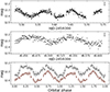 |
Fig. 1. Ks-band light curves derived from the NOT/NOTCAM photometry taken at 2021 March 31 (top panel) and 2021 May 5 (middle panel). Error bars on the right indicate the typical uncertainty, which is ≃0.025 mag in both cases. The bottom panel shows both light curves, phase-folded and phase-binned. Brown circles correspond to March 31, while grey squares represent May 5. To enhance clarity, the orbital cycle is repeated. |
3. Analysis and results
Multiple metallic absorption lines arising from the photosphere of the donor star are clearly visible in the K-band spectral range (Harrison 2016). The most prominent lines are the Na I doublet at ≃2.21 μm and the Ca I doublet at ≃2.26 μm, but there are also some weaker features, primarily from Ti I and Si I. All the spectroscopic measurements presented in this article were obtained in the wavelength ranges 2.09 − 2.11, 2.12 − 2.15 and 2.18 − 2.27 μm, which contain absorption features free from contamination from emission lines. Wavelengths > 2.27 μm were excluded from the analysis due to a significant drop in S/N. In the remainder of this paper, uncertainties are specified at the 68 per cent confidence level.
3.1. Radial velocity curve
We used the absorption lines of the donor star to derive its radial velocity curve by cross-correlating each YY Dra spectrum with the M2 V template Gl 797 B (see Sects. 3.2 and 3.3). Before cross-correlation, the template spectrum was corrected for its intrinsic radial velocity (determined by fitting the core of the Na I doublet at ≃2.21 μm with a double Gaussian), broadened to match the projected rotational velocity of the donor star (measured in Sect. 3.3), and rebinned onto the same logarithmic scale as the YY Dra spectra. The 2.4 km s−1 uncertainty in the wavelength calibration (Sect. 2) was quadratically added to the statistical error of each radial velocity measurement. As a validation, we repeated the measurements using the observed LHS 3558 template (M3 V) and found similar values within the errors for all the radial velocities.
We expect the photospheric lines to be affected by irradiation, with the impact on the radial velocities potentially changing from epoch to epoch due to long-term accretion variability. Consequently, we conducted analyses of our radial velocity curves for different epochs (see Table 1) with both circular and elliptical orbit fits. During this process, we treated all the data from 2022 May 12 and 17 as a single epoch due to the insufficient data points on each night to achieve successful fits separately. For the circular fit, we employed a sinusoidal equation for the radial velocity V(t):
![$$ \begin{aligned} V (t) = \gamma + K_{\mathrm{abs}} \, \mathrm{sin} \, \left[ \frac{2 \pi }{P}(t-T_{0}) \right] , \end{aligned} $$](/articles/aa/full_html/2024/10/aa51094-24/aa51094-24-eq4.gif)
where γ is the heliocentric systemic velocity, Kabs denotes the observed radial velocity semi-amplitude, P indicates the orbital period and T0 represents the time of closest approach of the donor star to the observer. For the elliptical fit, we used a second-order Fourier series of the form:

where x = 2π (t − T0)/P and the eccentricity is given by  for e ≤ 0.1 (see e.g. Martin et al. 1989).
In all fits, we fixed the orbital period and T0 according to the ephemeris given by Hill et al. (2022). Table 2 presents the best-fit parameters. Both the 2021 May and 2022 May data sets are well-fitted with a circular orbit, with χ2/dof close to 1 and Kabs ≃ 185 km s−1, where dof refers to the degrees of freedom of the fit. In addition, the resulting e value in the elliptical fit is either consistent or very close to null. In contrast, the 2020 February data set is not well-represented by the circular fit (χ2/dof > 2), and the e value from the elliptical fit appears larger (but consistent with 0 within the errors). This difference may be explained by a different irradiation level during our 2020 February observations. In this regard, YY Dra experienced a low state during which accretion greatly diminished approximately 5 days before our 2020 February observations (Hill et al. 2022) and the data from TESS show that it was increasing in brightness at the time of our spectroscopy.
Best-fit parameters of the circular and elliptical fits to the radial velocity measurements.
We completed our analysis of the radial velocity curve by combining the 2021 May and 2022 May data sets, since they gave similar fit parameters within the errors when treated separately. Figure 2 shows all the phase-folded radial velocities along with the best circular (solid line) and elliptical (dashed line) fits to the combined 2021 May + 2022 May data points. The elliptical fit results in a small but significant eccentricity, e = 0.03 ± 0.01. For this reason, the value of the radial velocity semi-amplitude of the donor star’s centre of mass, K2, will be presented in Sect. 3.4, where we concurrently model the 2021 May + 2022 May radial velocities and the light curves obtained from our NOT/NOTCAM photometry (Sect. 2.2). In this process, we take advantage of the partial simultaneity between the radial velocity measurements and the photometric data to model the irradiation.
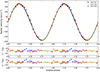 |
Fig. 2. Phase-folded heliocentric radial velocity curve of the donor star in YY Dra , obtained by cross-correlating our individual spectra of the target with the M2 V template spectrum Gl 797 B. The top panel shows the measured radial velocities along with the best circular (solid line) and elliptical (dashed line) fits. The middle panel displays the residuals from the circular fit, while the bottom panel represents those from the elliptical fit. The orbital cycle is shown twice for the sake of clarity. We excluded the 2020 February radial velocities from the fitting process. Data points from this epoch at phases 0.17 − 0.21 and 0.37 − 0.41 clearly exhibit different behaviour. |
3.2. Spectral classification of the donor star
Previous classifications of the donor star in YY Dra include: M3 V (Patterson et al. 1982), M3–M5.5 V (Mukai et al. 1990), M3 V (Friend et al. 1990) and M4 ± 1 V (Mateo et al. 1991). Additionally, Harrison (2016) finds the donor star to be consistent with a M1.8 dwarf with metallicity [Fe/H] = −0.20 dex using a single 240 s K-band spectrum with ≃135 km s−1 resolution at 2.2 μm. For this analysis, he employed empirical relationships of the equivalent width of absorption lines in M-dwarfs and comparison with synthetic templates. Taking advantage of our full orbital coverage, we decided to test these results by performing our classification of the donor star with two grids of spectral templates with different metallicities: one with −0.30 < [Fe/H] < 0.00 dex and another one with 0.00 < [Fe/H] < 0.30 dex. We will refer to them as the subsolar and supersolar metallicity grids, respectively. They were constructed from publicly available high S/N spectra of M-type dwarf stars in Rojas-Ayala et al. (2012). Their spectral resolution is R = λ/Δλ = 2700, which equates to ≃110 km s−1 resolution at 2.2 μm, close to the total broadening in the YY Dra data resulting from the convolution of the instrumental and rotational profiles (Sects. 2.1 and 3.3). Tables 3 and 4 list all the selected templates, providing their effective temperatures and [Fe/H] values.
Spectral classification of the donor star in YY Dra using the grid of subsolar metallicity templates.
For the spectral classification, we applied the optimal subtraction technique outlined in Marsh et al. (1994) combining all the YY Dra spectra, including the 2020 February dataset. This method optimises the subtraction of a scaled and broadened spectral template from the Doppler-corrected average spectrum of the target (see Fig. 3 for an illustration of the technique). We detail here how we proceeded with each of the templates. First, we velocity-shifted all YY Dra and template spectra to a common rest frame. Subsequently, we computed a weighted average of the YY Dra spectra, with weights proportional to the S/N. We then broadened the absorption lines of the template spectrum through convolution with Gray’s rotational profile (Gray 1992), adopting a linear limb-darkening coefficient of 0.19 for the K band, which is a plausible value for an early M-type star (Claret et al. 1995). The vrotsin i space was explored between 1 and 200 km s−1 in steps of 1 km s−1. To account for the fact that the donor star contributes a fraction, f, to the total flux in our wavelength range, the broadened versions of the template were multiplied by different f values > 0. Finally, all these broadened and scaled versions of the template were subtracted from the YY Dra average spectrum. The optimal values for the broadening and f are those that minimise the χ2 between the residual of the subtraction and a smoothed version of itself, obtained by convolution with a FWHM = 30 Å Gaussian. The minimum χ2/dof for each template is listed in Tables 3 and 4, and the top panel of Fig. 4 illustrates these results. The robust measurement of vrotsin i will be presented in Sect. 3.3, where we employ spectral type templates taken with the same instrumental setup as the YY Dra spectra.
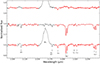 |
Fig. 3. Example of the application of the optimal subtraction technique. The order of the spectra, from bottom to top, is as follows: YY Dra average in the apparent rest frame of the donor star, Gl 402 template from Rojas-Ayala et al. (2012) broadened to match the YY Dra average, and the residual after subtraction of the broadened and scaled template. Red sections in the spectra indicate the wavelength regions used for the analysis. For clarity, the template and residual spectra have been vertically shifted. We mark the most important absorption lines according to the NASA IRTF spectral library atlas (Rayner et al. 2009). Optimal subtraction removes all lines of the donor star, except for the Ti I line at 2.1903 μm. This is also true for the other templates and in Harrison (2016), indicating that this difference is intrinsic to YY Dra. |
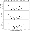 |
Fig. 4. Results from the spectral classification of the donor star in YY Dra using the optimal subtraction technique with the subsolar templates listed in Table 3 (squares) and the supersolar templates from Table 4 (triangles). The top panel shows the results for the full average spectrum of YY Dra, while the middle and bottom panels are for the averages at orbital phases 0.9 − 0.1 and 0.4 − 0.6, respectively. The relation between spectral type and effective temperature is illustrated at the top. |
Considering both grids as a whole, the χ2/dof exhibits a plateau between ≃3250 and ≃3700 K, corresponding to an spectral type range of M0.5–M3.5 according to the tabulation for main sequence stars by Pecaut & Mamajek (2013). In particular, the best-fit template has an effective temperature of ≃3530 K for both grids, corresponding to an M2 V star. This is in agreement with the M1.8 V classification by Harrison (2016), which comes from a single K-band spectrum taken at orbital phase 0.86. Nevertheless, UV/X-ray irradiation could result in an earlier spectral type in the donor’s dayside. To investigate this, we produced average spectra of YY Dra for orbital phases 0.9 − 0.1 (night hemisphere, 9 individual spectra) and 0.4 − 0.6 (day hemisphere, 10 individual spectra) and repeated the optimal subtraction procedure for both. The results are depicted in the middle and bottom panels of Fig. 4. In both cases, the preferred effective temperature range remains very similar, and the best-fit subsolar and supersolar templates align with that from the full average. This suggests that the temperatures of the day and night sides of the donor star must be quite close. We also searched for a narrow component in the Brγ emission line profiles coming from a heated hemisphere of the donor star, but it was not detected.
The f values fall in the ≃0.8 − 1.0 range. The best-matching templates in the supersolar grid (Table 4) exhibit deeper absorption lines, resulting in a lower f measurement compared to templates of similar effective temperatures in the subsolar grid (Table 3). The latter give f = 1 or even higher, which is not physically possible. Two features in our data make clear that f < 1: the flickering in the light curves (Fig. 1) and the presence of the Brγ emission line in the spectra (Fig. 3), with an equivalent width of −33 ± 7 Å (mean and standard deviation)6. Moreover, our modelling of the data (presented in Sect. 3.4) supports that the donor star contributes ≃80 − 85% to the K-band flux, in line with the values obtained with the best-fit templates with supersolar metallicity (Table 4). These arguments suggest that the metallicity of the donor star in YY Dra is probably higher than solar, in contrast with the [Fe/H] = −0.20 dex claimed by Harrison (2016). We attribute this disagreement to the fact that Harrison (2016) did not consider the reduction in the depth of the absorption lines produced by veiling. In fact, Harrison (2018) concludes that many of the CV spectra identified as having low metallicity in Harrison (2016) are probably affected by non-negligible veiling. In this context, Harrison (2018) obtains [Fe/H] = 0.0 dex for SS Cyg and RU Peg when accounting for the plausible veiling, while they were reported to have [Fe/H] = −0.3 dex in Harrison (2016).
3.3. Projected rotational velocity of the donor star
For the analysis in this section, we once again employed the optimal subtraction technique. This time we used the three spectral templates of M-type dwarfs obtained during our observational campaign: Gl 176, Gl 797 B and LHS 3558. The effective temperatures of these templates (see Table 5) are within the constraints found in Sect. 3.2 for the donor star of YY Dra. Since these templates are subject to the same instrumental broadening as the target spectra, using the optimal subtraction method with them allow us to achieve a robust measurement of vrotsin i. Prior to this, we simulated in our template spectra the impact of the radial velocity drift in the absorption lines during the length of the spectroscopic observations: for each template, we generated as many copies as the number of target spectra. Then, we applied to these copies the smearing suffered by the individual YY Dra spectra through convolution with a rectangular profile of the corresponding width, calculated from the effective length of the exposures and the orbital parameters. Finally, these smeared copies were averaged using identical weights as for the target spectra. The smearing correction is negligible: not applying it results in the exact same values and errors for vrotsin i and f.
vrotsin i and f values for YY Dra.
As part of the analysis, we examined the impact on the value of vrotsin i of the FWHM of the Gaussian employed to smooth the residual resulting from the optimal subtraction. We find that varying the FWHM between 1 and 50 Å implies changes in the value of vrotsin i below 5 km s−1, displaying a weak parabolic relationship with a minimum at ≃30 Å. Álvarez-Hernández et al. (2023) conducted tests on data taken with the same instrumental configuration that demonstrate that the minimum in the FWHM-broadening curves represents the actual vrotsin i. Consequently, we select the vrotsin i values derived using a 30-Å FWHM smoothing Gaussian.
To assess the uncertainties in vrotsin i and f, we employed the Monte Carlo procedure described in Steeghs & Jonker (2007) and Torres et al. (2020). We generated 10 000 bootstrapped copies of the average spectrum of YY Dra, repeating the optimal subtraction technique for each of them. This process yielded probability distributions for vrotsin i and f, both of which were effectively fitted by Gaussians. Therefore, in both cases, we adopted the mean and standard deviation as the representative value and the 1σ uncertainty, respectively.
Table 5 presents the vrotsin i and f values obtained using the three spectral templates. Their metallicities are in the range −0.23 ≤ [Fe/H] ≤ 0.15 dex, having a negligible effect on vrotsin i. The mean vrotsin i is 103 km s−1. For subsequent sections, we adopt this value while retaining the uncertainty of the individual measurements (103 ± 2 km s−1). This decision partially accounts for potential systematics introduced by the choice of the linear limb-darkening coefficient in Gray’s rotational profile (Gray 1992). In this respect, we have used a limb-darkening coefficient which is suitable for the continuum (Claret et al. 1995), but absorption lines in late-type stars have lower limb-darkening than the continuum (Collins & Truax 1995). Adopting the extreme case of zero limb-darkening changes the vrotsin i value by −1 km s−1.
The modulation of vrotsin i with orbital phase is well-documented (see e.g. Shahbaz et al. 2014). Our spectra of YY Dra cover the full orbital cycle with a consistently uniform sampling. As a result, the vrotsin i measurements provided above are expected to closely represent the mean value throughout the entire orbit. We verified this by checking that a consistent result (within 1σ agreement) is obtained when averaging the vrotsin i measurements at orbital phases 0.9 − 0.1, 0.15 − 0.35, 0.4 − 0.6, and 0.65 − 0.85.
3.4. Modelling of the light and radial velocity curves
To determine the fundamental parameters of YY Dra, we conducted simultaneous modelling of the two Ks-band light curves (Sect. 2.2) and the 2021 May + 2022 May radial velocities of the donor star (Sect. 3.1). We selected only these radial velocities since both of them exhibit a consistent behaviour (see the text in Sect. 3.1). All the curves were phase-folded using the ephemeris provided by Hill et al. (2022), and the light curves were averaged into 40 orbital phase bins, as shown in the bottom panel of Fig. 1. We used XRBCURVE, a code described in Shahbaz et al. (2000, 2003, 2017). The model considers a binary system composed of a primary star (assumed to be a point source) surrounded by an accretion disc and a co-rotating secondary star. The Roche lobe-filling factor of the latter can be specified, and we set it to 1. The accretion disc is circular and has a height H at the outer edge, and we adopted the circularization radius (Warner 1995) as the disc outer radius. We assumed that the accretion disc and the WD provide constant flux through the whole orbit, as no evidence of a hotspot or similar feature was found in the light curves (Sect. 2.2).
In the absence of irradiation, the flux of the donor star depends only on its unperturbed effective temperature (T2) and its limb- and gravity-darkening. We calculated its intensity distribution using NEXTGEN model-atmosphere fluxes (Hauschildt et al. 1999) and the tabulations by Claret & Bloemen (2011) for the limb- and gravity-darkening coefficients. To account for the irradiation of the donor star’s surface, we followed Shahbaz et al. (2003) and Shahbaz et al. (2017). Firstly, we computed the increase in the effective temperature for each surface element due to the UV/X-ray irradiation, adopting an UV/X-ray albedo of 0.5 for the donor star. Using albedo values of 0.1 and 1 produces consistent results within 1σ for all the parameters and changes ≲1 per cent in the derived masses7. Subsequently, we integrated the entire visible part of the donor star at each orbital phase to determine the total flux. For the radial velocity curve, the approach was similar: we used an equivalent width-effective temperature relation derived from PHOENIX model spectra (Husser et al. 2013) to establish the equivalent width of the absorption lines for each surface element based on its effective temperature. To account for the fact that absorption lines can disappear in surface elements that are subject to high irradiation levels, we introduced the limiting factor FAV. This represents the maximum fraction of total-to-unperturbed flux that a surface element can have while still maintaining the absorption features. For instance, if FAV = 1.50, the equivalent width of the lines is set to zero in the surface elements where the incident flux exceeds 50 per cent of the unperturbed flux. Finally, we integrated the entire visible part of the donor star at each orbital phase to determine the corresponding line-of-sight radial velocity.
The free parameters of the model include γ, K2, cos i, vrotsin i, T2, the distance to the source in parsecs (dpc) and the height-to-radius ratio of the accretion disc (H/R). Additionally, we parameterise the unabsorbed UV/X-ray heating flux of the WD for both the first ( ) and second (
 ) light curves, where the latter also represents the UV/X-ray flux for the radial velocity curve due to simultaneity. To properly model irradiation, FAV (described above) is another free parameter. The flux contribution to the Ks band from the WD and the accretion disc introduce two additional parameters, represented in terms of the donor star’s fractional contribution to the Ks-band flux, denoted as
  and
and  for the first and second light curves, respectively. Finally, the set of free parameters is completed by phase shifts of the synthetic curves with respect to the observed curves. These are δϕLC1 and δϕLC2 for the first and second light curves, respectively, and δϕRVC for the radial velocity curve. They account for uncertainties in the ephemeris and for potential differences between the spectroscopic and the photometric T0.
To simultaneously fit the two light curves and the radial velocity curve, we used a Markov chain Monte Carlo (MCMC) method convolved with a differential evolution fitting algorithm within a Bayesian framework (see Shahbaz et al. 2017 and references within). We utilised flat prior probability distributions for γ, K2, cos i, T2, H/R,  ,
,  , FAV,
  ,
,  , δϕLC1, δϕLC2 and δϕRVC. For T2, we employed the 3250 − 3700 K limits, according to the results from Sect. 3.2. We imposed Gaussian priors in vrotsin i and dpc based on our result from Sect. 3.3 and the distance from Bailer-Jones et al. (2021), respectively. We employed 60 walkers to explore the parameter space and 15 000 steps per chain, discarding the first 1000 as burn-in. The best simultaneous fit to the light and radial velocity curves is displayed in Fig. 5, while Fig. 6 presents the correlation plot. At each iteration, q was calculated using vrotsin i and K2 following equation 2 in Álvarez-Hernández et al. (2023), while the masses were derived from q, K2, i and P applying equations 5 and 6 in the same reference. The χ2 value for the simultaneous fit is 53.7 (dof = 97). Table 6 provides the resulting model parameters and the 1σ statistical uncertainties.
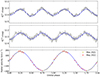 |
Fig. 5. Result of the simultaneous modelling of the light and radial velocity curves of YY Dra. From top to bottom: phase-binned Ks-band light curves from 2021 March 31 and May 5, followed by the radial velocity curve of the donor star (excluding the 2020 February data). The blue solid lines represent the best fit. The orbital cycle is shown twice for the sake of clarity. The fit of the first light curve (top panel) displays the absolute minimum at orbital phase 0.5, while it is at phase 0 in the fit of the second curve (middle panel) due to changes in irradiation ( |

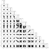 |
Fig. 6. Correlation diagrams illustrating the probability distributions resulting from the simultaneous modelling of the light and radial velocity curves of YY Dra using XRBCURVE. Only the most relevant parameters are shown. The 68, 95 and 99.7 per cent confidence contours are indicated in the 2D plots. In the right panels, the projected 1D parameter distributions are presented, with dashed lines indicating the mean and 68 per cent confidence level intervals. |
In our model, the accretion disc shadowing over the donor star surface is determined by the H/R ratio, for which we find a near uniform posterior. To evaluate if shadowing could have any impact on our calculations, we repeated the fit adopting a flat disc (H = 0), resulting in changes in the parameters ≲1 per cent. The result from this test alleviates the concerns about potential systematic errors induced by simplifying the geometry of the accretion structures in YY Dra to a disc. It also addresses the fact that shadowing may be lower due to the vertical extent of the irradiating regions. Moreover, shadowing only plays an important role in systems where irradiation is sufficiently high (see e.g. Shahbaz et al. 2019). In this regard, our model predicts changes < 20 K between the day and night hemispheres of the donor star, which is an indication of low heating. Accordingly, none of the surface elements reaches the best-fit limiting factor FAV (Table 6). We also find that there are not systematic errors introduced by our selection of the radial velocities for the modelling: using only the 2021 May velocities yields the same results (change ≲1 per cent) for all the parameters, while including the 2020 February data provides consistent values (within 1σ).
Best-fit parameters of the simultaneous modelling of the light and radial velocity curves using XRBCURVE.
The K2 derived from the modelling is  km s−1. For comparison, Mateo et al. (1991) obtained K2 = 184 ± 10 km s−1. To test our result, we followed Marsh (1988) and fitted a circular orbit to the radial velocities in the orbital phase range 0.8 − 1.2. We derived K2 = 188 ± 3 km s−1, which matches the value obtained from the modelling. The possible K2 > Kabs may be a consequence of irradiation being sufficient to increase the brightness of the day side without changing the spectral type. This shifts the centre of light of the absorption line spectrum towards the WD, as proposed to explain the radial velocity curve of SS Cyg when irradiation is low (Robinson et al. 1986; Bitner et al. 2007). The mass ratio is q = 0.62 ± 0.02, which significantly differs from the previously reported values of q = 0.48 ± 0.07 and q = 0.45 ± 0.05 presented in Mateo et al. (1991) and Haswell et al. (1997), respectively. These were derived from the ratio of radial velocity semi-amplitude of emission and absorption lines. In constrast, our value agrees with q = 0.61 ± 0.09, derived by Haswell et al. (1997) using the vrotsin i = 110 ± 10 km s−1 and KNa I = 202 ± 3 km s−1 measurements by Friend et al. (1990). The resulting cos i = 0.74 ± 0.02 yields i = 42°−1°+2°. This is consistent with previous estimates in the literature: i = 42° ±5° (Mateo et al. 1991), i = 45° ±4° (Haswell et al. 1997) and i = 41° ±3° (Joshi 2012). The derived binary masses are:
  ,
,  .
.
4. Discussion
4.1. Derived properties of the stellar components
The spectrum of the donor star in YY Dra is consistent with a spectral type M0.5–M3.5 V, most likely ≃M2 V (Sect. 3.2). This finding is supported by the previous classification of M1.8 V using the same spectroscopic band by Harrison (2016). The dynamical mass is 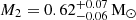 , and the Roche lobe volume radius can be calculated as
  . The surface gravity log g = 4.83 ± 0.06 dex derived from these quantities falls within the expected range for a dwarf star. According to Pecaut & Mamajek (2013)8, an M2 V star has a mass of ≃0.44 M⊙. This suggests that the donor star in YY Dra is more massive than expected for its spectral type, as observed in the dwarf nova IP Peg (P ≃ 3.80 h, Copperwheat et al. 2010) and the nova-like CVs HS 0220+0603 (P ≃ 3.58 h, Rodríguez-Gil et al. 2015) and KR Aur (P ≃ 3.91 h, Rodríguez-Gil et al. 2020). Higher masses have also been found in non-interacting dwarfs: there are robustly-classified M1-M3 V stars with accurately determined masses of ≃0.6 − 0.7 M⊙ (see e.g. Tables 2 and 5 in Torres et al. 2010).
Donor stars in CVs are supposed to be slightly oversized with respect to isolated main sequence stars of the same mass (see e.g. Patterson et al. 2005; Knigge 2006; Knigge et al. 2011). This is due to the thermal timescale, τTh, being similar to the mass-loss timescale, τML. Using our dynamical mass determination, the empirical mass–radius relation for donor stars in CVs derived by Knigge et al. (2011) indicates a radius of 0.64 ± 0.08 R⊙, which only agrees within 2 σ with our R2 value. Adopting that the accretion rate for YY Dra (≃3.5 × 10¹⁵ g s−1, Suleimanov et al. 2019) is equal to the donor mass-transfer rate, Ṁ2, we calculate τML ≃ M2/Ṁ2 ≃ 1.3 × 10¹⁰ yr and τTh ≃ G M22 / L2 R2 ≃ 6.7 × 10⁸ yr, where L2 = 4πσR22 T24. These numbers, together with the value of R2, suggest that the donor star in YY Dra is able to maintain thermal equilibrium in spite of the mass transfer. Similar conclusions have been drawn for IP Peg (Copperwheat et al. 2010) and HS 0220+0603 (Rodríguez-Gil et al. 2015) based on comparable reasoning.
For the WD, we derive a dynamical mass of  . This is significantly higher than the mean value of ≃0.6 M⊙ obtained spectroscopically from isolated WDs in the Sloan Digital Sky Survey (Kepler et al. 2016, 2019). However, accurate mass measurements of WDs in CVs suggest they are typically more massive than their isolated counterparts, with an average value of
  (Zorotovic et al. 2011; Pala et al. 2022). Our dynamical mass falls within 1 sigma with the latter.
4.2. Comparison of the dynamical WD mass with estimates from X-ray spectral studies
Numerous X-ray studies have provided estimates of the mass of WDs in IPs (hereafter M1X). The predominant approach for this is modelling the X-ray spectral continuum, as outlined in studies like Shaw et al. (2020), which relies on certain assumptions. Firstly, it assumes that the temperature of the plasma in the region where the accreted material impacts the WD surface is a function of the WD mass and radius (Aizu 1973). Secondly, the main cooling mechanism is presumed to be the emission of X-rays, specifically thermal bremsstrahlung (Wu et al. 1994; Cropper et al. 1998), although some authors have proposed comptonization as a possibility (e.g. Maiolino et al. 2021). Typically, this method is considered reliable when using hard (> 20 keV) X-ray spectra, as for masses > 0.6 M⊙, the maximum temperature exceeds 20 keV (Suleimanov et al. 2005). Moreover, the soft spectrum of many IPs is significantly affected by incompletely understood absorption and reflection components (Suleimanov et al. 2019). Fortunately, all the M1X values from X-ray spectral modelling that we have found in the literature for YY Dra were derived from hard X-ray data. Suleimanov et al. (2005) fitted a 3 − 100 keV RXTE/PCA+HEXTE spectrum using a multi-temperature bremsstrahlung model with the approximation of accreted matter falling from infinity, obtaining  . However, this result only agrees within the 2σ level with our dynamical measurement. Brunschweiger et al. (2009) employed the same model on 15 − 195 keV Swift/BAT data, obtaining a lower estimate,
  . They suggested that their value might be an underestimate due to the inappropriateness of the accreted matter falling from infinity assumption for systems with short spin periods. Yuasa et al. (2010) used a similar model with 3 − 50 keV Suzaku data and found
  , in agreement with our dynamical mass, but with high uncertainty. Using a comparable approach, Xu et al. (2019) modelled 0.3 − 50 keV Suzaku spectroscopy and derived
 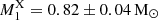 , which agrees within 2σ with our measurement. On the other hand, Suleimanov et al. (2019) used a more complex model considering a finite fall height for the accreted matter and fitted a 15 − 195 keV Swift/BAT spectrum, obtaining
 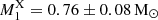 . This falls below our dynamical WD mass but remains within a 2σ agreement.
Other X-ray studies try to infer the WD mass from emission lines rather than fitting the spectral continuum. Xu et al. (2019) employed synthetic X-ray spectra to establish a relation between the ratio of the 6.7 and 7.0 keV iron emission lines and the WD mass. By measuring that ratio in Suzaku spectroscopy and applying their relation, they found 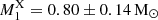 . This estimate shows a 1σ agreement with our dynamical mass.
In conclusion, the majority of M1X values derived from modelling of the hard X-ray spectral continuum are likely underestimates. The M1X obtained from the ratio of the 6.7 and 7.0 keV iron emission lines shows a 1σ agreement with the dynamical value, suggesting a potential correlation between that ratio and the WD mass. However, this method has not been tested against a significant number of dynamical masses. The only previous case is XY Ari, where the high uncertainty of the M1X value prevented any conclusion. Figure 7 provides a visual summary of the comparison conducted in this section. Our findings are consistent with those in Álvarez-Hernández et al. (2021) and Álvarez-Hernández et al. (2023), where a significant number of M1X values derived from modelling the hard X-ray spectral continuum of GK Per and XY Ari are found to be underestimates, even with refined models that consider the finite fall height of the accreted material onto the WD.
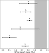 |
Fig. 7. Visual comparison of our dynamical WD mass for YY Dra (shaded column, 1 σ) with previous estimates derived from spectral modelling of: RXTE hard X-ray data (labelled in the figure as 1; Suleimanov et al. 2005), Swift hard X-ray data (labelled as 2 and 5; Brunschweiger et al. 2009 and Suleimanov et al. 2019) and Suzaku hard X-ray data (labelled as 3 and 4; Yuasa et al. 2010 and Xu et al. 2019). We also include one estimate based on the ratio of the iron emission lines in Suzaku spectroscopy (labelled as 6; Xu et al. 2019). |
5. Conclusions
We conducted a dynamical study of the IP YY Dra using partially simultaneous near-infrared spectroscopy and photometry taken between 2020 and 2022. We used the spectra to constrain the spectral type of the donor star to M0.5–M3-5 V, derive its radial velocity curve and measure the rotational broadening vrotsin i = 103 ± 2 km s−1. From the photometry, we derived two light curves, which we modelled together with the radial velocity curve. This analysis yielded the fundamental parameters of the system, including the radial velocity semi-amplitude of the centre of mass of the donor star  km s−1, the mass ratio q = 0.62 ± 0.02 and the orbital inclination i = 42−1°+2°. These results are consistent with previous estimates from the literature. The resulting dynamical masses for the WD and the donor star are
  and
and  , respectively. Compared to a typical main sequence star of the same spectral type, the donor star has a slightly larger mass, as observed in other CVs. Likewise, the WD mass aligns with the average value in CVs.
When comparing our dynamical WD mass with estimates from modelling of the hard X-ray spectral continuum, we find significant disagreements, in line with previous dynamical studies exploring this issue in other IPs. Additionally, we compared our value with one estimate derived from the ratio of X-ray iron emission lines, revealing good agreement. The latter may be an accurate technique; however, it warrants further testing to confirm it as a reliable method. This dynamical study provides another valuable piece of evidence to assess the accuracy of current X-ray methods in deriving WD masses for IPs.
A summary of the controversy regarding the name of YY Dra is available in The Catalog of IPs and IP Candidates by Koji Mukai: https://asd.gsfc.nasa.gov/Koji.Mukai/iphome/systems/yydra.html
For comparison, the equivalent width of the Brγ emission line is −14 ± 6 Å in the spectroscopy of XY Ari when f ≃ 0.7 − 0.8 in the K band (Álvarez-Hernández et al. 2023).
For zero albedo, the masses of the WD and the donor star increase by ≃5 per cent and ≃4 per cent, respectively. However, this has no impact on the discussion presented in Sect. 4.
Acknowledgments
We thank the anonymous referee for providing constructive suggestions. Based on observations made with the Gran Telescopio Canarias (GTC), installed at the Spanish Observatorio del Roque de los Muchachos of the Instituto de Astrofísica de Canarias, on the island of La Palma. This article is also based on observations made with the Nordic Optical Telescope, owned in collaboration by the University of Turku and Aarhus University, and operated jointly by Aarhus University, the University of Turku and the University of Oslo, representing Denmark, Finland and Norway, the University of Iceland and Stockholm University at the Observatorio del Roque de los Muchachos, La Palma, Spain, of the Instituto de Astrofisica de Canarias. We express our gratitude to the GTC staff, especially Antonio L. Cabrera Lavers, for their assistance in implementing the spectroscopy presented in this paper. Special thanks to Alina Streblyanska for sharing her expertise on EMIR with us. We also extend our thanks to Nicolás Cardiel López for clarifying certain aspects of PYEMIR. The use of the MOLLY package developed by Tom Marsh is acknowledged. This work was supported by the Agencia Estatal de Investigación del Ministerio de Ciencia e Innovación (MCIN/AEI) and the European Regional Development Fund (ERDF) under grant PID2021-124879NB-I00. MAPT acknowledges to have received support via a Ramón y Cajal Fellowship (RYC-2015-17854). PR-G acknowledges support from the Consejería de Economía, Conocimiento y Empleo del Gobierno de Canarias and the European Regional Development Fund (ERDF) under grant with reference ProID2021010132. P.G.J. has received funding from the European Research Council (ERC) under the European Union’s Horizon 2020 research and innovation programme (Grant agreement No. 101095973).
References
- Aizu, K. 1973, Prog. Theor. Phys., 49, 1184 [CrossRef] [Google Scholar]
- Álvarez-Hernández, A., Torres, M. A. P., Rodríguez-Gil, P., et al. 2021, MNRAS, 507, 5805 [CrossRef] [Google Scholar]
- Álvarez-Hernández, A., Torres, M. A. P., Rodríguez-Gil, P., et al. 2023, MNRAS, 524, 3314 [CrossRef] [Google Scholar]
- Andronov, I. L., & Mishevskiy, N. N. 2018, Res. Notes Am. Astron. Soc., 2, 197 [NASA ADS] [Google Scholar]
- Bailer-Jones, C. A. L., Rybizki, J., Fouesneau, M., Demleitner, M., & Andrae, R. 2021, AJ, 161, 147 [Google Scholar]
- Bitner, M. A., Robinson, E. L., & Behr, B. B. 2007, ApJ, 662, 564 [NASA ADS] [CrossRef] [Google Scholar]
- Brunschweiger, J., Greiner, J., Ajello, M., & Osborne, J. 2009, A&A, 496, 121 [NASA ADS] [CrossRef] [EDP Sciences] [Google Scholar]
- Cardiel, N., Pascual, S., Gallego, J., et al. 2019, ASP Conf. Ser., 523, 317 [NASA ADS] [Google Scholar]
- Chanmugam, G., & Wagner, R. L. 1977, ApJ, 213, L13 [NASA ADS] [CrossRef] [Google Scholar]
- Claret, A., & Bloemen, S. 2011, A&A, 529, A75 [NASA ADS] [CrossRef] [EDP Sciences] [Google Scholar]
- Claret, A., Diaz-Cordoves, J., & Gimenez, A. 1995, A&AS, 114, 247 [NASA ADS] [Google Scholar]
- Collins, G. W., I, & Truax, R. J. 1995, ApJ, 439, 860 [NASA ADS] [CrossRef] [Google Scholar]
- Copperwheat, C. M., Marsh, T. R., Dhillon, V. S., et al. 2010, MNRAS, 402, 1824 [Google Scholar]
- Covington, A. E., Shaw, A. W., Mukai, K., et al. 2022, ApJ, 928, 164 [NASA ADS] [CrossRef] [Google Scholar]
- Cropper, M. 1990, Space Sci. Rev., 54, 195 [CrossRef] [Google Scholar]
- Cropper, M., Ramsay, G., & Wu, K. 1998, MNRAS, 293, 222 [NASA ADS] [CrossRef] [Google Scholar]
- Cutri, R. M., Skrutskie, M. F., van Dyk, S., et al. 2003, VizieR Online Data Catalog: II/246 [Google Scholar]
- Friend, M. T., Martin, J. S., Smith, R. C., & Jones, D. H. P. 1990, MNRAS, 246, 637 [Google Scholar]
- Garzón, F., & EMIR Team 2016, ASP Conf. Ser., 507, 297 [Google Scholar]
- Garzón, F., Balcells, M., Gallego, J., et al. 2022, A&A, 667, A107 [CrossRef] [EDP Sciences] [Google Scholar]
- Gray, D. F. 1992, The Observation and Analysis of Stellar Photospheres (Cambridge: Cambridge University Press) [Google Scholar]
- Harrison, T. E. 2016, ApJ, 833, 14 [NASA ADS] [CrossRef] [Google Scholar]
- Harrison, T. E. 2018, ApJ, 861, 102 [NASA ADS] [CrossRef] [Google Scholar]
- Haswell, C. A., Patterson, J., Thorstensen, J. R., Hellier, C., & Skillman, D. R. 1997, ApJ, 476, 847 [NASA ADS] [CrossRef] [Google Scholar]
- Hauschildt, P. H., Allard, F., & Baron, E. 1999, ApJ, 512, 377 [Google Scholar]
- Henden, A. A., & Honeycutt, R. K. 1995, PASP, 107, 324 [NASA ADS] [CrossRef] [Google Scholar]
- Hill, K. L., Littlefield, C., Garnavich, P., et al. 2022, AJ, 163, 246 [NASA ADS] [CrossRef] [Google Scholar]
- Husser, T. O., Wende-von Berg, S., Dreizler, S., et al. 2013, A&A, 553, A6 [NASA ADS] [CrossRef] [EDP Sciences] [Google Scholar]
- Joshi, V. 2012, PhD Thesis, Gujarat University, India [Google Scholar]
- Kepler, S. O., Pelisoli, I., Koester, D., et al. 2016, MNRAS, 455, 3413 [NASA ADS] [CrossRef] [Google Scholar]
- Kepler, S. O., Pelisoli, I., Koester, D., et al. 2019, MNRAS, 486, 2169 [NASA ADS] [Google Scholar]
- Knigge, C. 2006, MNRAS, 373, 484 [NASA ADS] [CrossRef] [Google Scholar]
- Knigge, C., Baraffe, I., & Patterson, J. 2011, ApJS, 194, 28 [Google Scholar]
- Maiolino, T., Titarchuk, L., Wang, W., Frontera, F., & Orlandini, M. 2021, ApJ, 911, 80 [NASA ADS] [CrossRef] [Google Scholar]
- Marsh, T. R. 1988, MNRAS, 231, 1117 [CrossRef] [Google Scholar]
- Marsh, T. R., Robinson, E. L., & Wood, J. H. 1994, MNRAS, 266, 137 [NASA ADS] [CrossRef] [Google Scholar]
- Martin, J. S., Friend, M. T., Smith, R. C., & Jones, D. H. P. 1989, MNRAS, 240, 519 [CrossRef] [Google Scholar]
- Mateo, M., Szkody, P., & Garnavich, P. 1991, ApJ, 370, 370 [NASA ADS] [CrossRef] [Google Scholar]
- Mukai, K., Mason, K. O., Howell, S. B., et al. 1990, MNRAS, 245, 385 [NASA ADS] [Google Scholar]
- Pala, A. F., Gänsicke, B. T., Belloni, D., et al. 2022, MNRAS, 510, 6110 [NASA ADS] [CrossRef] [Google Scholar]
- Patterson, J. 1994, PASP, 106, 209 [Google Scholar]
- Patterson, J., Schwartz, D. A., Bradt, H., et al. 1982, BAAS, 14, 618 [NASA ADS] [Google Scholar]
- Patterson, J., Schwartz, D. A., Pye, J. P., et al. 1992, ApJ, 392, 233 [NASA ADS] [CrossRef] [Google Scholar]
- Patterson, J., Kemp, J., Harvey, D. A., et al. 2005, PASP, 117, 1204 [Google Scholar]
- Pecaut, M. J., & Mamajek, E. E. 2013, ApJS, 208, 9 [Google Scholar]
- Rayner, J. T., Cushing, M. C., & Vacca, W. D. 2009, ApJS, 185, 289 [Google Scholar]
- Robinson, E. L., Zhang, E. H., & Stover, R. J. 1986, ApJ, 305, 732 [NASA ADS] [CrossRef] [Google Scholar]
- Rodríguez-Gil, P., Shahbaz, T., Marsh, T. R., et al. 2015, MNRAS, 452, 146 [CrossRef] [Google Scholar]
- Rodríguez-Gil, P., Shahbaz, T., Torres, M. A. P., et al. 2020, MNRAS, 494, 425 [CrossRef] [Google Scholar]
- Rojas-Ayala, B., Covey, K. R., Muirhead, P. S., & Lloyd, J. P. 2012, ApJ, 748, 93 [Google Scholar]
- Shahbaz, T., Groot, P., Phillips, S. N., et al. 2000, MNRAS, 314, 747 [NASA ADS] [CrossRef] [Google Scholar]
- Shahbaz, T., Zurita, C., Casares, J., et al. 2003, ApJ, 585, 443 [NASA ADS] [CrossRef] [Google Scholar]
- Shahbaz, T., Watson, C. A., & Dhillon, V. S. 2014, MNRAS, 440, 504 [NASA ADS] [CrossRef] [Google Scholar]
- Shahbaz, T., Linares, M., & Breton, R. P. 2017, MNRAS, 472, 4287 [CrossRef] [Google Scholar]
- Shahbaz, T., Linares, M., Rodríguez-Gil, P., & Casares, J. 2019, MNRAS, 488, 198 [NASA ADS] [CrossRef] [Google Scholar]
- Shaw, A. W., Heinke, C. O., Mukai, K., et al. 2020, MNRAS, 498, 3457 [NASA ADS] [CrossRef] [Google Scholar]
- Smette, A., Sana, H., Noll, S., et al. 2015, A&A, 576, A77 [NASA ADS] [CrossRef] [EDP Sciences] [Google Scholar]
- Steeghs, D., & Jonker, P. G. 2007, ApJ, 669, L85 [NASA ADS] [CrossRef] [Google Scholar]
- Suleimanov, V., Revnivtsev, M., & Ritter, H. 2005, A&A, 435, 191 [NASA ADS] [CrossRef] [EDP Sciences] [Google Scholar]
- Suleimanov, V. F., Doroshenko, V., & Werner, K. 2019, MNRAS, 482, 3622 [NASA ADS] [CrossRef] [Google Scholar]
- Szkody, P., Nishikida, K., Erb, D., et al. 2002, AJ, 123, 413 [NASA ADS] [CrossRef] [Google Scholar]
- Torres, G., Andersen, J., & Giménez, A. 2010, A&ARv, 18, 67 [Google Scholar]
- Torres, M. A. P., Casares, J., Jiménez-Ibarra, F., et al. 2020, ApJ, 893, L37 [NASA ADS] [CrossRef] [Google Scholar]
- Šimon, V. 2000, A&A, 360, 627 [NASA ADS] [Google Scholar]
- Warner, B. 1995, Camb. Astrophys. Ser., 28 [Google Scholar]
- Williams, G. 1983, ApJS, 53, 523 [NASA ADS] [CrossRef] [Google Scholar]
- Wilson, R. E., Devinney, E. J., & Van Hamme, W. 2020, Astrophysics Source Code Library [record ascl:2004.004] [Google Scholar]
- Wu, K., Chanmugam, G., & Shaviv, G. 1994, ApJ, 426, 664 [NASA ADS] [CrossRef] [Google Scholar]
- Xu, X.-J., Yu, Z.-L., & Li, X.-D. 2019, ApJ, 878, 53 [NASA ADS] [CrossRef] [Google Scholar]
- Yuasa, T., Nakazawa, K., Makishima, K., et al. 2010, A&A, 520, A25 [NASA ADS] [CrossRef] [EDP Sciences] [Google Scholar]
- Zorotovic, M., Schreiber, M. R., & Gänsicke, B. T. 2011, A&A, 536, A42 [NASA ADS] [CrossRef] [EDP Sciences] [Google Scholar]
All Tables
Best-fit parameters of the circular and elliptical fits to the radial velocity measurements.
Spectral classification of the donor star in YY Dra using the grid of subsolar metallicity templates.
Best-fit parameters of the simultaneous modelling of the light and radial velocity curves using XRBCURVE.
All Figures
|
Fig. 1. Ks-band light curves derived from the NOT/NOTCAM photometry taken at 2021 March 31 (top panel) and 2021 May 5 (middle panel). Error bars on the right indicate the typical uncertainty, which is ≃0.025 mag in both cases. The bottom panel shows both light curves, phase-folded and phase-binned. Brown circles correspond to March 31, while grey squares represent May 5. To enhance clarity, the orbital cycle is repeated. |
| In the text | |
|
Fig. 2. Phase-folded heliocentric radial velocity curve of the donor star in YY Dra , obtained by cross-correlating our individual spectra of the target with the M2 V template spectrum Gl 797 B. The top panel shows the measured radial velocities along with the best circular (solid line) and elliptical (dashed line) fits. The middle panel displays the residuals from the circular fit, while the bottom panel represents those from the elliptical fit. The orbital cycle is shown twice for the sake of clarity. We excluded the 2020 February radial velocities from the fitting process. Data points from this epoch at phases 0.17 − 0.21 and 0.37 − 0.41 clearly exhibit different behaviour. |
| In the text | |
|
Fig. 3. Example of the application of the optimal subtraction technique. The order of the spectra, from bottom to top, is as follows: YY Dra average in the apparent rest frame of the donor star, Gl 402 template from Rojas-Ayala et al. (2012) broadened to match the YY Dra average, and the residual after subtraction of the broadened and scaled template. Red sections in the spectra indicate the wavelength regions used for the analysis. For clarity, the template and residual spectra have been vertically shifted. We mark the most important absorption lines according to the NASA IRTF spectral library atlas (Rayner et al. 2009). Optimal subtraction removes all lines of the donor star, except for the Ti I line at 2.1903 μm. This is also true for the other templates and in Harrison (2016), indicating that this difference is intrinsic to YY Dra. |
| In the text | |
|
Fig. 4. Results from the spectral classification of the donor star in YY Dra using the optimal subtraction technique with the subsolar templates listed in Table 3 (squares) and the supersolar templates from Table 4 (triangles). The top panel shows the results for the full average spectrum of YY Dra, while the middle and bottom panels are for the averages at orbital phases 0.9 − 0.1 and 0.4 − 0.6, respectively. The relation between spectral type and effective temperature is illustrated at the top. |
| In the text | |
|
Fig. 5. Result of the simultaneous modelling of the light and radial velocity curves of YY Dra. From top to bottom: phase-binned Ks-band light curves from 2021 March 31 and May 5, followed by the radial velocity curve of the donor star (excluding the 2020 February data). The blue solid lines represent the best fit. The orbital cycle is shown twice for the sake of clarity. The fit of the first light curve (top panel) displays the absolute minimum at orbital phase 0.5, while it is at phase 0 in the fit of the second curve (middle panel) due to changes in irradiation ( |
| In the text | |
|
Fig. 6. Correlation diagrams illustrating the probability distributions resulting from the simultaneous modelling of the light and radial velocity curves of YY Dra using XRBCURVE. Only the most relevant parameters are shown. The 68, 95 and 99.7 per cent confidence contours are indicated in the 2D plots. In the right panels, the projected 1D parameter distributions are presented, with dashed lines indicating the mean and 68 per cent confidence level intervals. |
| In the text | |
|
Fig. 7. Visual comparison of our dynamical WD mass for YY Dra (shaded column, 1 σ) with previous estimates derived from spectral modelling of: RXTE hard X-ray data (labelled in the figure as 1; Suleimanov et al. 2005), Swift hard X-ray data (labelled as 2 and 5; Brunschweiger et al. 2009 and Suleimanov et al. 2019) and Suzaku hard X-ray data (labelled as 3 and 4; Yuasa et al. 2010 and Xu et al. 2019). We also include one estimate based on the ratio of the iron emission lines in Suzaku spectroscopy (labelled as 6; Xu et al. 2019). |
| In the text | |
Current usage metrics show cumulative count of Article Views (full-text article views including HTML views, PDF and ePub downloads, according to the available data) and Abstracts Views on Vision4Press platform.
Data correspond to usage on the plateform after 2015. The current usage metrics is available 48-96 hours after online publication and is updated daily on week days.
Initial download of the metrics may take a while.