| Issue |
A&A
Volume 690, October 2024
|
|
|---|---|---|
| Article Number | A8 | |
| Number of page(s) | 12 | |
| Section | The Sun and the Heliosphere | |
| DOI | https://doi.org/10.1051/0004-6361/202451016 | |
| Published online | 25 September 2024 | |
Testing the volume integrals of travel-time sensitivity kernels for flows
1
Astronomical Institute, Charles University, Faculty of Mathematics and Physics, V Holešovičkách 2, CZ-18000 Prague, Czech Republic
2
Astronomical Institute of the Czech Academy of Sciences, Fričova 298, CZ-25165 Ondřejov, Czech Republic
Received:
7
June
2024
Accepted:
12
July
2024
Context. Helioseismic inversions largely rely on sensitivity kernels, in which 3D spatial functions describe how the changes in the solar interior translate into the change in helioseismic observables. These sensitivity kernels in most cases come from the forward modelling that is used in the most advanced solar models.
Aims. We aim to test the sensitivity kernels by comparing their volume integrals with measured values from helioseismic travel times.
Methods. By manipulating the tracking rate, we mimicked the additional zonal velocity in the Dopplergram datacubes. These datacubes were then processed by a standard travel-time measurements pipeline. We investigated the dependence of the east-west travel time averaged over a box around the disc centre on the implanted tracking velocity. The slope of this dependence is directly proportional to the total volume integral of the sensitivity kernel that corresponds to the travel-time geometry that is used.
Results. The agreement between measurements and models for travel times that are computed with a ridge filtering is very good to acceptable. The dependence we sought to determine indeed resembles a linear function, and its slope agrees with the expected volume integral from the forward-modelled sensitivity kernel. The agreement is poorer for the phase-speed filtered datacubes. The disagreement is particularly strong for the slowest phase speeds (filters td1–td4). For the higher phase speeds, our result indicates that the measured kernel integrals are systematically larger than expected from the forward modelling. We admit our testing procedure may not be appropriate for high phase speeds and higher radial modes.
Key words: Sun: helioseismology / Sun: oscillations
© The Authors 2024
 Open Access article, published by EDP Sciences, under the terms of the Creative Commons Attribution License (https://creativecommons.org/licenses/by/4.0), which permits unrestricted use, distribution, and reproduction in any medium, provided the original work is properly cited.
This article is published in open access under the Subscribe to Open model. Subscribe to A&A to support open access publication.
1. Introduction
The photospheric layers of the Sun are optically thick, which prevents us from directly studying the interior of our mother star. In the past seven decades, some of the information hiding below the impenetrable solar skin may have serendipitously been revealed indirectly with the helioseismic method.
Helioseismology (Gizon & Birch 2005; Basu 2016) in general encompasses a set of methods that enable us to examine the inner composition and dynamics of the Sun through the analysis of solar oscillations. Many aspects of the solar interior structure have been successfully revealed through helioseismology, such as the depth of the convection zone, the character of the rotation of the convective envelope, the global meridional mass circulation, or indications of a pre-emergence of active regions.
Helioseismology is based on the observation and interpretation of the manifestations of seismic waves that propagate through the interior. These waves are excited near the solar surface, likely by the vigorous convection within solar granules. The travel path (in the first approximation) is determined by the 1D structure of the Sun. Perturbations in this background structure cause the waves to deviate in propagation and change speed (Christensen-Dalsgaard 2008). The waves manifest themselves in some surface observables, such as the continuum intensity, or in Doppler shifts and the line depths of photospheric spectral lines and others. They are best seen in the above mentioned Doppler shifts. Hence, current helioseismic instruments record spatially resolved Doppler shifts of a particular photospheric spectral line, the Dopplergrams. The sequence of the Dopplergrams that records dynamical changes at a particular spatial position is then processed in order to learn about the behaviour of the solar seismic waves. These Dopplergram sequences are available for instance from the Michelson Doppler Imager (MDI; Scherrer et al. 1995) or from the Helioseismic and Magnetic Imager (HMI; Scherrer et al. 2012; Schou et al. 2012 instruments.
A specific approach called local helioseismology (see a review by Gizon et al. 2010) focuses on observation and analysis of the waves in a spatially limited region. The wave field within the chosen region is influenced by the properties of that particular area at the surface and beneath it. Consequently, by analysing the wave patterns in this local region, it becomes possible to deduce local 3D structures and dynamics beneath the surface (Christensen-Dalsgaard 2002). The standard procedure used in all methods of local helioseismology involves selecting a small region on the solar surface and tracking it within a co-rotation frame, that is, the region does not move in time relative to the surface of the Sun.
A specific method of local helioseismology, the time-distance helioseismology (Duvall 1993), studies the travel times of the waves that are tracked when they travel between two places on the Sun. In its simplicity, the travel time τ is measured between two measurement points (pixels) in the surface measurements, r1 and r2. We indicate a helioseismic observable (e.g. a sequence of Dopplergrams that might be even filtered) at these points as Ψ(r1, t) and Ψ(r2, t). The key mathematical quantity to be evaluated is then the cross-covariance, which is evaluated as

in its discrete form (Gizon & Birch 2002). Here, ht is the temporal sampling, and T is the duration of the observation.
In realistic applications, the cross-covariance function that is measured for two points contains much realisation noise that is due to the stochastic nature of solar oscillations. Hence, it is almost impossible to measure the travel time of the waves that travel between two individual pixels in the helioseismic observables. Some averaging is usually required. Most often, this averaging is applied both in time and space. In time, cross-covariances are usually averaged over a time period T longer than about 6 hours. To further improve the signal-to-noise ratio, it was first suggested by Duvall (1993) to average the cross-covariance C(r1, r2, t) over points r2 that belong to the annulus or quadrants centred at r1 with a distance Δ = |r2 − r1|. To study the waves travelling from the central point towards the surrounding annulus and in the opposite direction, averaging over a full annulus is suitable. To investigate the waves that travel in the direction parallel to the equator (east-west), an averaging over 90-degree quadrants of the annulus in the corresponding direction is more suitable. In the method used in this study, quadrants were replaced by sections of the annulus multiplied by the cosine (east-west direction) or sine (south-north direction) of the horizontal polar angle. These geometries constitute a continuous transition from quadrant geometries.
For a given set of r1 and Δ, the cross-covariance function oscillates around a characteristic travel time in both the positive and negative part of the time axis. It is a goal of the time-distance methods to search for the travel time that maximises the cross-covariance (1). One of the approaches to measuring the travel time is to fit a Gaussian wavelet to the cross-covariance function (Kosovichev & Duvall 1997),
![$$ \begin{aligned} C_+(t; \mathbf r _1,\Delta ) = A\exp [ - {\gamma ^2}{(t - {t_{\rm {g}}})^2}]\cos [{\omega _0}(t - {\tau _+})], \end{aligned} $$](/articles/aa/full_html/2024/10/aa51016-24/aa51016-24-eq2.gif)
where A is the amplitude, tg represents the group travel time, and τ+ is the positive phase travel time. Parameters A and γ describe the amplitude and decay rate of the wavelet envelope. An analogous equation may be written for a negative travel time. The time-distance analysis relies on the measurement and interpretation of the phase travel times τ+ and τ−.
The fitting of the Gaussian wavelet is demanding and often fails due to the presence of noise. Therefore, alternative definitions of travel times were developed that are more robust in the presence of noise. They stem from the fact that the cross-covariance of the waves may be computed from the solar model by solving the equations of the wave propagation. These cross-covariances represent some sort of a reference for a spherically symmetrical 1D quiet Sun. We can safely assume that the changes to the cross-covariances caused by the perturbations of the model introduce a modification of the background-model cross-covariances. Then, instead of fitting a five-parameter Gaussian wavelet, this reference cross-covariance can be used as a template, and only a one-parameter fitting in time is required. This approach is also used in geoseismology (Zhao & Jordan 1998), and for the need of time-distance helioseismology, it was devised by Gizon & Birch (2002). Following this paper, we refer to these travel times as to GB02 travel times henceforth. In this approach, not the full travel time τ is measured, but the deviation δτ of the travel time from the reference template.
Gizon & Birch (2004) later simplified this definition even further for the case of small perturbations. This robust definition allows the measurement of travel times averaged over a short time (e.g. around T = 2 hours) and with a high spatial resolution. This linearised approach is called GB04 henceforth.
We note that the GB02 and GB04 definitions of the travel times both result in a travel time that is a mixture of the group and phase travel times. It is not straightforward to decouple the two. A proper choice of the reference cross-covariance C0 is essential to minimise the contribution of the group travel time to the results. In some cases, a reference cross-covariance from the forward modelling may not be accurate enough. In these cases, the construction of the reference cross-covariance as a spatial average of different realisations over the field of view in the quiet-Sun regions may be a better choice.
We considered that the solar model is fully described by a multidimensional vector of quantities Qα(x), where the index α lists the considered physical quantities. These quantities can, for instance, be vector flows, the sound speed, the density, or the adiabatic exponent. In our study, we primarily focused on the flows v. The quantities Qα are functions of 3D spatial coordinates x and, in principle, also of time. However, we only considered stationary models in terms of the averaging over the observation interval T.
Similarly to the discussion of the travel times, the values of the quantities can be split into the unperturbed background Q0α(x), which in most cases is represented by the background solar model, and the perturbation qα(x).
To compute the linear adiabatic oscillations of the Sun, methods have been available for a very long time (Lynden-Bell & Ostriker 1967). This computation is slow and expensive even for the computational power of current computers. This approach is not viable for realistic problems. When we focus on linear perturbations of the model alone, we can relate travel-time deviations δτ with perturbations of the solar model qα by the equation

The index a represents the travel-time geometry and combines the choice of the k − ω filter, point-to-annulus, or point-to-quadrant averaging, and the radius of the annulus Δ. The measured travel times are subject to random realisation noise na. The quantity Kαa is called a sensitivity kernel and represents a function that translates changes in the solar model into travel-time deviations. The assumption of small perturbations allows us to split the total travel-time deviation into individual contributions by individual perturbers α.
The sensitivity kernel functions are calculated numerically using the background solar model. Various approaches have been developed by different authors. The simplest approximation ignores the finite-wavelength effects and assumes that the waves propagate along their optimal rays (see Kosovichev & Duvall 1997, and references therein). Finite-wavelength effects are considered by approximating the wave propagation in terms of scattering. Single-source sensitivity kernels were proposed and computed, for example, by Birch & Kosovichev (2000). Sensitivity kernels considering randomly distributed sources were proposed and developed by Gizon & Birch (2002). Later, a linearised approach consistent with the definition of linearised travel times was proposed by Gizon & Birch (2004). Gizon and Birch emphasised the importance of incorporating data processing steps (not only the k − ω filtering, but also an accurate estimate of the telescope point spread function) into the calculation of the kernels and ensuring that they align with the measured travel times. For details of the kernel calculation, we refer to Burston et al. (2015).
It needs to be mentioned that there are other more sophisticated methods that allow the computation of sensitivity kernels, namely the adjoint method (Hanasoge et al. 2011). The method relies on the computation of the wave field that is driven by two sources. One source is the excitation spectrum resulting in the forward wavefield, and the other source is the difference between the predicted wavefield and observations (the adjoint wavefield). The method thus minimises the misfit between the modelled and observed wavefield, whereas the sensitivity kernels are produced naturally within the process.
2. Motivation for this work
In real applications, the problem is usually posed in the opposite direction: We wish to learn from the measured travel-time maps about the properties of the solar interior, and therefore, we usually wish to invert (3) to infer qα. Not to mention issues with the chosen inversion schemes used by the community, the procedure critically depends on the accuracy of the sensitivity kernels. The kernels represent the background model of the Sun, around which the problem is linearised and solved. If the kernels were problematic, the recovered tomographic maps of the solar interior would also be affected by these issues.
Recently, one of us indicated inconsistencies in the special type of inversions for flows, where the technique of ensemble averaging was applied (Švanda 2015). This technique uses the assumption that when many realisation of the same phenomenon are averaged (it was the supergranular cells in that case), the averaging decreases the noise term in Eq. (3). In the inversion procedure, the term containing the sensitivity kernels is then of the most importance, and the results of the statistical inversion are constrained by these kernels alone. The study showed that various choices of sensitivity kernels in the inversion lead to very different models of the average supergranule. It was not possible to tell from the results and travel times alone which of the models was better, that is, closer to reality.
A similar issue was subsequently confirmed by DeGrave & Jackiewicz (2015), who showed that the observed travel-time maps are inconsistent with the forward-modelled travel times using various supergranular models. Their study directly tested Eq. (3) and pointed out possible issues with the kernels.
On the other hand, Duvall (2006) directly measured sensitivity kernels for flows for the surface gravity modes using small magnetic points as scatterers and obtained a reasonable match with the models.
A direct validation of the sensitivity kernels with observations is not possible. It is possible to test the kernels with respect to the Sun-like magnetohydrodynamic simulations, but most of the available simulations are not exactly Sun-like in terms of the properties of the surface flows and spectrum of solar oscillations. This motivated us to test at least some of the properties of the kernels with observations.
3. Testing procedure
The aim of this study is to test the validity of velocity (flow) perturbation sensitivity kernel integrals with a model-independent method. As a tool, we injected an artificial constant longitudinal flow (velocity perturbation) v0 into data from observations. This was achieved by tracking the selected region on the solar disc with a (known) constant velocity different from the solar rotation. This effectively means that to all perturbations qα mentioned in Eq. (3), an additional perturbation v0 representing the constant injected velocity was added, transforming the equation into
![$$ \begin{aligned} \delta \tau ^a(\mathbf r ) = \sum \limits _\alpha \int _{\odot }\mathrm{d^2}\mathbf{r ^{\prime }}\mathrm{d}{z}\mathbf K _\alpha ^a(\mathbf r ^{\prime } - \mathbf r , z) \cdot [ q^\alpha (\mathbf r ^{\prime }, z) - \mathbf v _0] + n^a(\mathbf r )\ . \end{aligned} $$](/articles/aa/full_html/2024/10/aa51016-24/aa51016-24-eq4.gif)
The minus sign in the term [qα(r′,z)−v0] arises because we injected the artificial flow by moving the coordinate frame. However, moving the frame in one direction corresponds to an apparent flow of the same velocity, but in the opposite direction, similarly to watching a landscape passing by through the window of a moving train. The term with v0 in the integrand is bound with a corresponding vector sensitivity kernel where Kva. Since v0 is constant and independent of position, it is not affected by the volume integral and can be taken out of it,
Strictly speaking, the additional velocity v0 should not be mistaken for the change in the rotational rate of the reference frame because it is constant with depth. A constant angular velocity corresponding to a different rate of solar rotation would manifest itself with a decreasing tangential velocity with depth. At the surface, the two approaches are equal. However, most of the time-distance kernels we have at our disposal are sensitive only in a depth of a few Mm below the surface, hence the inaccuracies from exchanging these two points of view in an interpretation of v0 in Eq. (5) are negligible. What is not negligible at all is the contribution of the random-noise realisation na. It also is not known a priori. One of the ways to suppress this term is by means of spatial averaging. At the position of neighbouring pixels, the random realisation is correlated (e.g. Gizon & Birch 2004), but the correlation length-scale, on the other hand, is only a few pixels. By averaging over many pixels (100×100 in our case), the contribution of the random noise is therefore significantly lowered.
Equation (5) then becomes

where angle brackets indicate the spatial averaging. The first term on the right side of Eq. (6) can be viewed as a certain average background travel-time perturbation that is unaffected by the implanted velocity. The second term is independent of position, and therefore, the averaging does not affect it and it remains unchanged. The average travel-time perturbation in a selected central area of the tracked region is clearly directly proportional to the volume integral of the velocity perturbation kernel, with the injected velocity acting as a constant of proportionality. The injected velocity has only a longitudinal (east-west, usually called vx) component. East-west quadrant-like difference travel times are most sensitive to this type of perturbation (Burston et al. 2015). Then, finally,

By applying a set of implanted velocities v0, we can independently measure the spatial integral of the sensitivity kernel Kvxa using a simple linear fit stemming from Eq. (7).
4. Data and methods
4.1. Data
The travel times were measured from a series of Dopplergram datacubes. The Dopplergrams were observed by the HMI instrument and stored within the Joint Science Operations Center (JSOC1). HMI scans the FeI 617.3 nm photospheric absorption line at six positions and measures the intensity across different polarisation states. The Dopplergrams were computed using a fast MDI-like algorithm (Couvidat et al. 2012) that employs the use of the discrete approximations of the Fourier coefficients describing the spectral line and correction by factors from pre-computed look-up tables. The final data products are stored within the series hmi.V_45s at JSOC, from which they are read by our pipelines using a module in the SUNPY package.
4.2. Tracking pipeline
The tracking pipeline is responsible for preparing datacubes that are then used for measuring the travel times. We wrote a versatile pipeline from scratch using routines from the SUNPY (SunPy Community et al. 2020) package so that it exactly matched our needs. In addition to the traditional steps such as selecting the local area, applying the azimuthal equidistant (Postel) projection, and creating the datacube in FITS format with a correct header, this pipeline offers an additional feature specific to this work: it implants artificial velocities by apparently moving the selected area at a predefined speed. This is a crucial feature used to determine the model-independent velocity kernel integrals as explained in previous sections. Since this is not part of standard pipelines for datacube preparation, our own solution was necessary.
The pipeline is highly versatile and prepared to be executed both on a single computer and in a cluster environment. Individual consecutive steps were written as separate modules, so that the user can verify the outcome of each step before proceeding further. At a high level, the tracking pipeline performs the steps listed below.
-
Prepare the folder structure together with all necessary configuration files (for the datacube creation step and for the subsequent travel-time pipeline) based on the input configuration (JSOC Data Record Management System (DRMS) queries, data paths, projection origins, and implanted velocities).
-
(OPTIONAL) Download data (Dopplergrams) from JSOC. This step is unnecessary when the required data are already downloaded.
-
Create a datacube for each combination of DRMS query and velocity and save it in the form of a FITS file into its designated folder prepared in step 1.
The configuration of the pipeline is given in the form of a text file. Among others, it contains the DRMS request string specifying the time range to be downloaded and processed, the positions of the centre of the tracked region in Carrington coordinates, lower and upper limits for implanted velocities, and the velocity sample count. The set of implanted velocities is then randomly sampled from within the given velocity bounds. Subsequently, a loop is executed over the realisation of the implanted velocities. Within this loop, the full-disc Dopplergrams are downloaded (they are downloaded only once for the given DRMS query), tracked and mapped following the requests, and stacked to a datacube.
Before a final saving into an FITS file with headers compatible with the following processing, invalid values (NaNs or blank pixels) are removed from the datacube frames and replaced by a median of non-empty values. Then, from each frame, a quadratic smooth surface is removed to subtract large-scale trends in Dopplergrams. A large-scale trend that smoothly varies across the field of view is naturally produced by the solar rotation, for instance.
One potential question is whether the injected longitudinal velocity truly results in an artificial flow within the data. To address this, ring diagrams were constructed from the datacube power spectrum that show that the rings are shifted in the datacubes with an implanted velocity with respect to the situation in the datacube that was tracked with the solar rotation (see Fig. 1). It qualitatively demonstrates the presence of a horizontal flow in the east-west direction, as evidenced by the horizontal distortion of the rings.
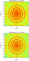 |
Fig. 1. Cuts through the power spectra at a frequency of 4 mHz in the datacube that was tracked with solar rotation (upper panel) and the same datacube tracked 500 m/s faster than solar rotation. The distortion of the rings due to the artificial velocity is clearly visible. |
A direct comparison of the horizontal velocity with the injected velocity is also possible. In the Dopplergrams, large-scale convective cells of supergranulation (Rincon & Rieutord 2018) are clearly visible. The supergranular structures can therefore be used to determine the horizontal flow field on the solar surface (e.g. Švanda et al. 2006, and the follow-up papers). This goal may be achieved by applying the method of local correlation tracking (LCT; November 1986) to Dopplergram datacubes.
The local correlation tracking algorithm searches for the optimal displacement that minimises the differences of the floating spatial windows that capture slowly evolving features in the time sequence. Knowing the sampling of the cross-correlated frames, we can convert the detected displacement into the horizontal velocity vector. In the test performed here, the horizontal velocity vector is dominated by the longitudinal component, which is the only one we compare with the implanted velocity.
The results of our pipeline test are shown in Fig. 2. The measured surface horizontal velocities clearly correspond very well to the implanted velocity, and thereby validate the performance of the tracking pipeline.
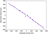 |
Fig. 2. Comparison of the implanted velocity and the longitudinal component of the horizontal velocity vector determined from the manipulated datacubes using the LCT algorithm. The fit has a slope of −1, which is a consequence of the fact that the implanted velocity was injected by artificially changing the reference frame, which naturally introduced an apparent flow in the opposite direction. |
4.3. Travel-time pipeline
In general, measurements of helioseismic travel times consist of three consecutive steps. The travel-time pipeline operated on the data-processing computer cluster at the Astronomical Institute of the Czech Academy of Sciences in Ondejov is no exception. First, the input datacube, that is, the output of the tracking pipeline, is detrended in time, and a mean frame (average of the frames over time) is subtracted. This step removes existing large-scale trends in the observations. In Dopplergrams, these large-scale trends may be produced by a residual signal from the differential rotation, for instance, and also by long-living velocity features, such as most of the signal from solar supergranules. The detrended datacube is apodised in both space and time and transformed into Fourier space for further processing.
The Fourier-transformed datacube is filtered to keep only certain types of waves. We use two types of filtering that are traditional in time-distance helioseismology, that is, the ridge filters (isolating only the surface gravity f modes or acoustic p-modes to the fourth order) and the phase-speed time-distance filters (indicated as td1 to td11, following Duvall 1997).
These filtered datacubes are inputs for the travel-time measurements procedure. Following the usual recipes, cross-covariance maps are computed numerically (see Equation (1)) for spatially smoothed datacubes using the generalised point-to-annulus geometry. Then, the travel times that minimise the cross-covariance of the signals at the given point are measured using a user-selected definition. In our case, we used both the GB02 and the GB04 definition.
This workflow was implemented in a pipeline coded in the MATLAB language. Each of the three steps is represented in a separate module, and the pipeline is executed in the cluster environment.
4.4. Sensitivity kernels
The sensitivity kernels that were tested were computed in the KC3 code by Aaron Birch (Birch & Gizon 2007). The code uses a mode summation approach in Cartesian geometry and a Born approximation with randomly distributed sources. It uses eigenfunctions and eigenfrequencies of the oscillations from the solar model S (Christensen-Dalsgaard et al. 1996). KC3 is a reference kernel code that produced sensitivity kernels for flow or sound-speed perturbation that were used in many studies before.
5. Results
To achieve the goals of this study, we analysed 716 separate datacubes in total. An overview is given in Table 1. The processed data volume consisted of 705 GB in the Dopplergram datacubes and 8.5 TB in the resulting travel-time maps and necessary intermediate data products. The processing took about two months using the Radegast cluster at the Solar Department of the Astronomical Institute of the Czech Academy of Sciences in Ondřejov, which has 102 CPU cores in total.
Summary table of the analysed datacubes.
For each ridge filter (f and p1 to p4 modes), we evaluated the travel times for 16 different distances Δ, starting at 5 px and ending at 20 px, with a pixel size of 1.46 Mm. The reason for the degraded MDI-like resolution is that the sensitivity kernels we have at our disposal and that we regularly use for helioseismic inversions within our group (e.g. Švanda et al. 2013; Švanda 2013; Švanda et al. 2014; Korda & Švanda 2019, 2021) have exactly this pixel size. As for the phase-speed filters td1 to td11, we used five distances Δ for each, following the usual definition of these filters by Couvidat & Birch (2006) (also Table 1 in Švanda 2013). For each mode (filter) and distance, we calculated travel-time maps for all three point-to-annulus and point-to-quadrant geometries. In the following, we only used the east-west averaging geometry, because it is most sensitive to the zonal flows (Burston et al. 2015) that we introduced artificially. Hence, we verified kernel integrals for 135 different sensitivity kernels in total.
The procedure is demonstrated for example in Fig. 3. There, for a chosen sensitivity kernel (index a), we plot the dependence given by Eq. (7), that is, the dependence of the average travel-time deviation in the central region ⟨δτa(r)⟩ of the datacube as a function of the implanted zonal velocity v0. The dependence is monotonous (this is the case for all considered as) and very close to linear, as expected. For higher values of v0 above around 300 m/s the average travel times start to deviate slightly from the linear fit, which is also over-plotted. This non-linearity is expected for high velocities and is consistent with previous works (see e.g. Jackiewicz et al. 2007). Therefore, we evaluated the fit of the linear function only in the range of ( − 300, +300) m/s. For higher modes (e.g. p4) and higher phase speeds, the non-linearity is slightly more pronounced. Following Eq. (7), the slope of the linear fit corresponds to the total spatial integral of the corresponding sensitivity kernel.
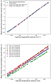 |
Fig. 3. Measured average travel time around the disc centre as a function of the implanted velocity. Top: Plot for mode td4 at a distance of 9.9 px. The linear fit and its properties are also indicated. The slope of the linear fit corresponds to the total integral of the appropriate sensitivity kernel. Bottom: Similar plot for the p3 mode and Δ = 15 px when using several dates. Different dates are grouped around virtual lines that are shifted vertically, as indicated by the time stamps. |
For the different dates, a different realisation of the background travel-time term ⟨δτbacka(r)⟩ in (Eq. 7) occurs (see Fig. 3 bottom panel). For instance, an uncorrected differential rotation contributes to this term. This term changes the intercept of the linear dependence. We are only interested in the slopes. In order to learn about the characteristic slope value, we fitted the linear dependence individually for each date and then obtained the representative slope value s as a weighted average,

where si are the individual slopes with their error bars σs, i.
The comparison of the resulting slope that represents the model-independent value of the total spatial integral of the sensitivity kernel with the value from the forward modelling for all modes and all distances is plotted in Fig. 4. The colours represent different modes, and the total integral values usually increase with the distance Δ. An expected line with a slope of −1 is over-plotted for reference.
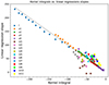 |
Fig. 4. Volume integrals of the velocity perturbation kernels obtained from linear regression slopes (model independent) vs. volume integrals of the velocity perturbation kernels calculated from forward modelling. The data were obtained from 578 different datacubes for various ridge and phase-speed filters. The dashed line indicates the expected line with a slope of −1. The values on both axes are in units of s/(km/s). |
The figure shows that the measured and modelled travel-time sensitivity kernel integrals correspond to each other for most of the ridge filters. This is also demonstrated further in Table 2, where the slopes for the f and p1 to p4 modes are close to the expected value of −1. The fits show a small spread, low intercept values, and a large (anti)correlation, and they are statistically significant. The slope deviates from −1 for the p4 mode, which penetrates to deeper layers, where the assumption of implanting the surface velocity that is applicable to the whole sub-surface region no longer holds.
Properties of the linear fits.
The situation is different for the phase-speed filters (see e.g. Fig. 5). Even when the correlation coefficient is close to −1 and the fits are significant (all cases except for td1 and perhaps td4, when we take the level of statistical significance 0.01), the slopes differ significantly from the expected value of −1. Moreover, the values of the intercepts are mostly high. The most notable differences occur for low phase speeds, for filters td1 to td5, for instance. Large deviations from the expectations are registered also for the highest phase speeds (filters td9 to td11), where the slope is much larger than the expected value. Some of this disagreement is probably due to the reason described above when discussing the p4 mode. On the other hand, p-modes with low phase speeds only penetrate shallow near-surface layers, and our testing approach should be valid for them.
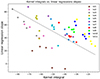 |
Fig. 5. Same as Fig. 4 with details of phase-speed filtered kernels. Moreover, this plot is obtained for a particular date, not for a combination of several dates. The dashed line indicates the expected line with a slope of −1. The values on both axes are in units of s/(km/s). |
We note that the linear fits by mode are rather indicative. A complete set of kernel integrals from the forward modelling and their comparison to the model-independent determination is given in Table A.1.
6. Discussion
Our results indicate an unresolved issue with the travel-time sensitivity kernels using phase-speed filtering. Some of the disagreement might be a consequence of the chosen testing procedure, where the implanted velocity is under control only at the surface. Deeper down, its proper interpretation becomes more difficult. The waves with high phase speeds and higher modes are more sensitive to the state of deeper modes. This property is prominent especially for the phase-speed-filtered waves (see e.g. Fig. 2 in Švanda 2013). Therefore, it is difficult to properly interpret the disagreement between the modelled and observed travel-time sensitivity kernel integrals for these modes. On the other hand, the disagreement is also present for very shallow waves (short distances in ridge-filtered data and lowest phase-speed filtered data with modes td1 to td4), where high-degree modes prevail. The disagreement of amplitudes and line widths of the models for the high-degree modes with the observations is known from the literature (see e.g. Korzennik et al. 2013), which affects the Green functions and cross-covariance functions used in the kernel models, among others.
It would seem at the first glance that the different conclusions drawn for ridge- and phase-speed-filtered kernels might indicate different approaches taken in processing the ridge- and phase-speed-filtered data. We wish to stress that this is not the case. In our testing procedure, an identical kernel code and an identical travel-time pipeline was used to process different filtering approaches. The corresponding k − ω filters are supplied to the code as external files with the same format. Both codes and pipelines are written in the programming language MATLAB and share as many common sub-routines as necessary. We would like to stress that our travel times and sensitivity kernels are mutually consistent in terms of the considered data-processing steps. Filtering, spatial resolutions, and so on are taken into account consistently in both the computation of the sensitivity kernels and measuring the travel times.
There is a handfull of choices in running the travel-time pipeline that might possibly influence the results of the presented comparison.
Choice of the travel-time fitting method. Our travel-time pipeline offers three definitions in total of the travel time to be used: Gabor-wavelet fitting, GB02, and GB04. We only used GB02 and GB04 in this study because our travel-time sensitivity kernels are compatible with these definitions. We tested that both approaches provided essentially indistinguishable results for implanted velocities in the range of about ( − 200, 200) m/s, then non-linearities started to appear for GB04 definition for some travel-time geometries. This is expected because the GB04 definition is only valid for small perturbations. For the GB04 definition, the points start to deviate from the linear fit sooner than shown in Fig. 3, for example, which was computed with the GB02 definition. For this reason, we preferred the GB02 definition for our final results even though it is significantly more demanding computationally. It allowed a wider range of the implanted velocities to be examined.
Averaging time. Averaging of the cross-covariances over a longer time span leads to a lower contribution of the random noise; the signal-to-noise ratio scales approximately as  with T being an averaging time. We computed several testing runs using T = 24 hours and T = 6 hours and compared the results. Averaging of the travel times in the spatial window around the centre of the tracked patch (we used 100 × 100 px window) is much more effective in suppressing the random noise than the choice of the longer averaging time. The averaging time therefore has no effect on the results of this study.
Choice of the reference cross-covariance. The GB02 and GB04 definitions of the travel times rely heavily on the reference cross-covariance that is used as a template to determine the offset δτ of the measured travel time. As pointed out already in the introduction, the reference cross-covariance should be close to the measured one. In the case of low implanted velocities, a usual quiet-Sun reference cross-covariance may be used, for instance the one from the forward modelling. With increasing v0, the deviations from the template became significant and break the assumption of the perturbation, which is a small change. When the surface is tracked at a rate that differs significantly from the background solar rotation, even the position of the emergent point changes, which again influences the measured cross-covariance when applying the non-modified pipeline. For a wave travelling about 20 minutes from the central point to the surrounding annulus (which is a characteristic time of the propagation in our choice of the waves), for example, the emergent point shifts by about 600 km with a tracking speed of 500 m/s with respect to the background solar rotation. This is about 0.4 pixels, which may already play a role in the measurement procedure.
We found that the use of the pre-computed cross-covariance from the solar model is insufficient to represent the changes introduced by the tracking. The use of the reference cross-covariance computed as an average over all representations in the field of view solves the issue.
Heliographic latitude. The results presented above were obtained with datacubes whose centres were positioned on the solar equator. We also ran the same procedure for two datacubes that were located at heliographic latitudes of +20 and −20 degrees. The results were very similar and only differed by the value of the intercept on the implanted velocity versus averaged travel time plot (see Fig. 3). The shift of the intercepts is a consequence of the differential rotation, which is not compensated for, as the basic rotation rate was the Carrington rotation rate. The comparisons between the measured sensitivity kernel integrals and the models were comparable to those presented in Table 2.
Other travel-time geometries. We focused primarily on the east-west geometry from the point-to-quadrant choices because it is naturally sensitive to the implanted zonal velocity (Burston et al. 2015). Other geometries, such as the point-to-annulus (also known as out-minus-in) or south-north geometry, can be used. The volume integrals of these geometries are zero for the zonal (vx) velocity. Therefore, the averaged travel times around the disc centre have a low value and vary quasi-randomly with implanted velocity (see Fig. 6).
7. Concluding remarks
We tested the volume integrals of the time-distance sensitivity kernels for flows and pointed out a possible issue in the sensitivity kernels that use the phase-speed filtering scheme. We need to stress that our study does not necessarily have to invalidate results and interpretations of the published helioseismic inversions in the past for the reasons listed below.
-
This test represents a form of a necessary condition sensitivity kernels should fulfil, but not a sufficient condition, as the procedure only tested the volume integrals of the kernels.
-
The disagreement of the total volume integral may lie in details that might in fact be marginal for a proper analysis. For instance, if there is a slight disagreement of the kernel value at pixels that are far from the central point and if this disagreement has a large area even when the difference is small, it will affect the total integral by a large amount due to the 2D integration.
-
Similarly, a shifted mean horizontal value will behave in the same way. A small shift but over a large area will significantly affect the total integral of the sensitivity kernel.
-
Švanda (2015) speculated that the reason of the inconsistency of the flow models derived from the inversion using different combinations of travel-time geometries was that during the inversion, the contributions of some kernels were cancelled by contributions from the others. The subtraction to zero critically depends on precise values, and when the values have small errors, the results are largely unconstrained. When the combination leads to the summation of the kernels, these results should be more robust in the presence of inconsistencies. If this hypothesis were to be true, the inversion schemes call for a method for determining the optimal combination of the sensitivity kernels that are to be used in the scheme that would avoid large-scale subtractions.
-
Comparisons between different codes for computing the sensitivity kernels were made in the past (e.g. Parchevsky et al. 2010; Böning et al. 2016), and they resulted in a generally good match between different techniques. The disagreement between various codes was to within a few percent. Even the comparison of the total integrals (Parchevsky et al. 2010) of kernels using very different wave-field approximations (ray approximation vs. Born approximation) showed an acceptable agreement. It should be possible with the numbers in Table A.1 to verify the kernel integrals also using other codes, provided that the data processing involved in the kernel computation is consistent with the travel-time measurements presented in this study.
-
We would also like to point out that except for the phase-speed filters td1–td4, the measured kernel integrals are somewhat proportional to the values obtained from the forward models (see Fig. 5). This is merely an observation, and no conclusion is drawn from it at the moment.
Many of the helioseismic inferences were achieved using methods involving sensitivity kernels. Our test indicates that there might be an issue with some of them, and therefore, more work on verification and validation is needed. Some helioseismic methods do not require sensitivity kernels and use the full waveform information about the solar oscillations (see e.g. Woodard 2007; Hanson et al. 2021; Mani et al. 2022; Hanson et al. 2024).
Acknowledgments
This paper presents the results obtained within completing the MSc. studies of D.Ch. under the supervision of M.Š. at the Faculty of Mathematics and Physics, Charles University. This work was partly done with a support of the institutional support ASU:67985815 of the Czech Academy of Sciences. M.Š. further acknowledges the support by Czech-German common grant, funded by the Czech Science Foundation under the project 23-07633K and by the Deutsche Forschungsgemeinschaft under the project BE 5771/3-1 (eBer23-13412). We are grateful to Aaron Birch for making his kernel code free to use.
References
- Basu, S. 2016, Liv. Rev. Sol. Phys., 13, 2 [Google Scholar]
- Birch, A. C., & Gizon, L. 2007, Astron. Nachr., 328, 228 [Google Scholar]
- Birch, A. C., & Kosovichev, A. G. 2000, Sol. Phys., 192, 193 [NASA ADS] [CrossRef] [Google Scholar]
- Böning, V. G. A., Roth, M., Zima, W., Birch, A. C., & Gizon, L. 2016, ApJ, 824, 49 [Google Scholar]
- Burston, R., Gizon, L., & Birch, A. C. 2015, Space Sci. Rev., 196, 201 [Google Scholar]
- Christensen-Dalsgaard, J. 2002, Rev. Mod. Phys., 74, 1073 [Google Scholar]
- Christensen-Dalsgaard, J. 2008, Lecture Notes on Stellar Structure and Evolution (Aarhus Universitet. Institute for Fysik og Astronomi) [Google Scholar]
- Christensen-Dalsgaard, J., Dappen, W., Ajukov, S. V., et al. 1996, Science, 272, 1286 [Google Scholar]
- Couvidat, S., & Birch, A. 2006, Sol. Phys., 237, 229 [NASA ADS] [CrossRef] [Google Scholar]
- Couvidat, S., Rajaguru, S. P., Wachter, R., et al. 2012, Sol. Phys., 278, 217 [NASA ADS] [CrossRef] [Google Scholar]
- DeGrave, K., & Jackiewicz, J. 2015, Sol. Phys., 290, 1547 [Google Scholar]
- Duvall, T. L. J., Jefferies, S. M., Harvey, J. W., & Pomerantz, M. A., 1993, Nature, 362, 430 [CrossRef] [Google Scholar]
- Duvall, T. L. J., Kosovichev, A. G., Scherrer, P. H., et al. 1997, Sol. Phys., 170, 63 [NASA ADS] [CrossRef] [Google Scholar]
- Duvall, T. L. J., Birch, A. C., & Gizon, L., 2006, ApJ, 646, 553 [NASA ADS] [CrossRef] [Google Scholar]
- Gizon, L., & Birch, A. 2002, ApJ, 571, 966 [NASA ADS] [CrossRef] [Google Scholar]
- Gizon, L., & Birch, A. 2004, ApJ, 614, 472 [NASA ADS] [CrossRef] [Google Scholar]
- Gizon, L., & Birch, A. C. 2005, Liv. Rev. Sol. Phys., 2, 6 [Google Scholar]
- Gizon, L., Birch, A. C., & Spruit, H. C. 2010, ARA&A, 48, 289 [Google Scholar]
- Hanasoge, S. M., Birch, A., Gizon, L., & Tromp, J. 2011, ApJ, 738, 100 [NASA ADS] [CrossRef] [Google Scholar]
- Hanson, C. S., Hanasoge, S., & Sreenivasan, K. R. 2021, ApJ, 910, 156 [NASA ADS] [CrossRef] [Google Scholar]
- Hanson, C. S., Bharati Das, S., Mani, P., Hanasoge, S., & Sreenivasan, K. R. 2024, Nat. Astron., in press, https://doi.org/10.1038/s41550-024-02304-w [Google Scholar]
- Jackiewicz, J., Gizon, L., Birch, A. C., Duvall, T. L. J., 2007, ApJ, 671, 1051 [NASA ADS] [CrossRef] [Google Scholar]
- Korda, D., & Švanda, M. 2019, A&A, 622, A163 [NASA ADS] [CrossRef] [EDP Sciences] [Google Scholar]
- Korda, D., & Švanda, M. 2021, A&A, 646, A184 [NASA ADS] [CrossRef] [EDP Sciences] [Google Scholar]
- Korzennik, S. G., Rabello-Soares, M. C., Schou, J., & Larson, T. P. 2013, ApJ, 772, 87 [NASA ADS] [CrossRef] [Google Scholar]
- Kosovichev, A. G., Duvall, T. L. J., 1997, Astrophys. Space Sci. Lib., 25, 241 [NASA ADS] [CrossRef] [Google Scholar]
- Lynden-Bell, D., & Ostriker, J. P. 1967, MNRAS, 136, 293 [Google Scholar]
- Mani, P., Hanson, C. S., & Hanasoge, S. 2022, ApJ, 926, 127 [NASA ADS] [CrossRef] [Google Scholar]
- November, L. J. 1986, Appl. Opt., 25, 392 [CrossRef] [Google Scholar]
- Parchevsky, K., Birch, A., Kosovichev, A., et al. 2010, Am. Astron. Soc. Meeting Abstr., 216, 400.09 [NASA ADS] [Google Scholar]
- Rincon, F., & Rieutord, M. 2018, Liv. Rev. Sol. Phys., 15, 6 [Google Scholar]
- Scherrer, P. H., Bogart, R. S., Bush, R. I., et al. 1995, Sol. Phys., 162, 129 [Google Scholar]
- Scherrer, P. H., Schou, J., Bush, R. I., et al. 2012, Sol. Phys., 275, 207 [Google Scholar]
- Schou, J., Scherrer, P. H., Bush, R. I., et al. 2012, Sol. Phys., 275, 229 [Google Scholar]
- SunPy Community, Barnes, W. T., Bobra, M. G., et al. 2020, ApJ, 890, 68 [NASA ADS] [CrossRef] [Google Scholar]
- Švanda, M. 2013, ApJ, 775, 7 [Google Scholar]
- Švanda, M. 2015, A&A, 575, A122 [NASA ADS] [CrossRef] [EDP Sciences] [Google Scholar]
- Švanda, M., Klvaňa, M., & Sobotka, M. 2006, A&A, 458, 301 [NASA ADS] [CrossRef] [EDP Sciences] [Google Scholar]
- Švanda, M., Roudier, T., Rieutord, M., Burston, R., & Gizon, L. 2013, ApJ, 771, 32 [Google Scholar]
- Švanda, M., Sobotka, M., & Bárta, T. 2014, ApJ, 790, 135 [Google Scholar]
- Woodard, M. F. 2007, ApJ, 668, 1189 [NASA ADS] [CrossRef] [Google Scholar]
- Zhao, L., & Jordan, T. H. 1998, Geophys. J. Int., 133, 683 [NASA ADS] [CrossRef] [Google Scholar]
Appendix A: All investigated kernels
Comparison table of modelled and inferred volume integrals for all considered travel-time kernels.
All Tables
Comparison table of modelled and inferred volume integrals for all considered travel-time kernels.
All Figures
|
Fig. 1. Cuts through the power spectra at a frequency of 4 mHz in the datacube that was tracked with solar rotation (upper panel) and the same datacube tracked 500 m/s faster than solar rotation. The distortion of the rings due to the artificial velocity is clearly visible. |
| In the text | |
|
Fig. 2. Comparison of the implanted velocity and the longitudinal component of the horizontal velocity vector determined from the manipulated datacubes using the LCT algorithm. The fit has a slope of −1, which is a consequence of the fact that the implanted velocity was injected by artificially changing the reference frame, which naturally introduced an apparent flow in the opposite direction. |
| In the text | |
|
Fig. 3. Measured average travel time around the disc centre as a function of the implanted velocity. Top: Plot for mode td4 at a distance of 9.9 px. The linear fit and its properties are also indicated. The slope of the linear fit corresponds to the total integral of the appropriate sensitivity kernel. Bottom: Similar plot for the p3 mode and Δ = 15 px when using several dates. Different dates are grouped around virtual lines that are shifted vertically, as indicated by the time stamps. |
| In the text | |
|
Fig. 4. Volume integrals of the velocity perturbation kernels obtained from linear regression slopes (model independent) vs. volume integrals of the velocity perturbation kernels calculated from forward modelling. The data were obtained from 578 different datacubes for various ridge and phase-speed filters. The dashed line indicates the expected line with a slope of −1. The values on both axes are in units of s/(km/s). |
| In the text | |
|
Fig. 5. Same as Fig. 4 with details of phase-speed filtered kernels. Moreover, this plot is obtained for a particular date, not for a combination of several dates. The dashed line indicates the expected line with a slope of −1. The values on both axes are in units of s/(km/s). |
| In the text | |
 |
Fig. 6. Figure similar to Fig. 3, but for the f mode, point-to-annulus geometry with Δ = 11 px. |
| In the text | |
Current usage metrics show cumulative count of Article Views (full-text article views including HTML views, PDF and ePub downloads, according to the available data) and Abstracts Views on Vision4Press platform.
Data correspond to usage on the plateform after 2015. The current usage metrics is available 48-96 hours after online publication and is updated daily on week days.
Initial download of the metrics may take a while.