| Issue |
A&A
Volume 690, October 2024
|
|
|---|---|---|
| Article Number | A144 | |
| Number of page(s) | 10 | |
| Section | Galactic structure, stellar clusters and populations | |
| DOI | https://doi.org/10.1051/0004-6361/202450531 | |
| Published online | 04 October 2024 | |
The boring history of Gaia BH3 from isolated binary evolution
1
Physics and Astronomy Department Galileo Galilei, University of Padova,
Vicolo dell’Osservatorio 3,
35122,
Padova,
Italy
2
INFN – Padova,
Via Marzolo 8,
35131
Padova,
Italy
3
INAF – Padova,
Vicolo dell’Osservatorio 5,
35122
Padova,
Italy
4
Institut für Theoretische Astrophysik, ZAH, Universität Heidelberg,
Albert-Ueberle-Straße 2,
69120
Heidelberg,
Germany
5
Niels Bohr International Academy, Niels Bohr Institute,
Blegdamsvej 17,
2100
Copenhagen,
Denmark
6
Departament de Física Quàntica i Astrofísica, Institut de Ciències del Cosmos, Universitat de Barcelona,
Martí i Franquès 1,
08028
Barcelona,
Spain
7
SISSA,
via Bonomea 365,
34136
Trieste,
Italy
8
Univ Lyon, Univ Lyon1, ENS de Lyon, CNRS, Centre de Recherche Astrophysique de Lyon UMR5574,
69230
Saint-Genis-Laval,
France
9
INAF, Osservatorio Astronomico di Bologna,
Via Gobetti 93/3,
40129
Bologna,
Italy
10
Gran Sasso Science Institute,
Via F. Crispi 7,
67100
L’Aquila,
Italy
11
INFN – Laboratori Nazionali del Gran Sasso,
67100
L’Aquila,
Italy
12
INAF – Osservatorio Astronomico d’Abruzzo,
Via Mentore Maggini, s.n.c.,
64100
Teramo,
Italy
★ Corresponding authors; This email address is being protected from spambots. You need JavaScript enabled to view it.
; This email address is being protected from spambots. You need JavaScript enabled to view it.
; This email address is being protected from spambots. You need JavaScript enabled to view it.
Received:
26
April
2024
Accepted:
31
July
2024
Abstract
Gaia BH3 is the first observed dormant black hole (BH) with a mass of ≈30 M⊙, and it represents the first confirmation that such massive BHs are associated with metal-poor stars. Here, we explore the isolated binary formation channel for Gaia BH3, focusing on the old and metal-poor stellar population of the Milky Way halo. We used the MIST stellar models and our open-source population synthesis code SEVN to evolve 5.6 × 10⁸ binaries, exploring 20 sets of parameters that encompass different natal kicks, metallicities, common envelope efficiencies and binding energies, and models for the Roche-lobe overflow. We find that systems such as Gaia BH3 form preferentially from binaries initially composed of a massive star (40–60 M⊙) and a low-mass companion (<1 M⊙) in a wide (P > 103 days) and eccentric orbit (e > 0.6). Such progenitor binary stars do not undergo any Roche-lobe overflow episode during their entire evolution, so the final orbital properties of the BH-star system are essentially determined at the core collapse of the primary star. Low natal kicks (≲ 10 km/s) significantly favour the formation of Gaia BH3-like systems, but high velocity kicks up to ≈220 km/s are also allowed. We estimated the formation efficiency for Gaia BH3-like systems in old (t >10 Gyr) and metal-poor (Z < 0.01) populations to be ∼4 × 10⁻⁸ M⊙−1 (for our fiducial model), representing ~3% of the whole simulated BH-star population. We expect up to ≈4000 BH-star systems in the Galactic halo formed through isolated evolution, of which ≈100 are compatible with Gaia BH3. Gaia BH3-like systems represent a common product of isolated binary evolution at low metallicity (Z < 0.01), but given the steep density profile of the Galactic halo, we do not expect more than one at the observed distance of Gaia BH3. Our models show that even if it was born inside a stellar cluster, Gaia BH3 is compatible with a primordial binary star that escaped from its parent cluster without experiencing significant dynamical interactions.
Key words: methods: numerical / binaries: general / stars: black holes / stars: massive / Galaxy: halo / Galaxy: stellar content
© The Authors 2024
 Open Access article, published by EDP Sciences, under the terms of the Creative Commons Attribution License (https://creativecommons.org/licenses/by/4.0), which permits unrestricted use, distribution, and reproduction in any medium, provided the original work is properly cited.
This article is published in open access under the Subscribe to Open model. This email address is being protected from spambots. You need JavaScript enabled to view it. to support open access publication.
1 Introduction
Gaia data (Gaia Collaboration 2023) offer a unique opportunity to search for dormant black holes (BHs), that is X-ray and radio-quiet BHs that are members of a binary system with a star (Guseinov & Zel’dovich 1966; Trimble & Thorne 1969). Gaia BH3, the third dormant BH retrieved from these data, has a mass of ≈33 M⊙ and is member of a loose eccentric binary system (orbital period P≈4000 days, eccentricity e ≈ 0.72) that includes a ≈0.76 M⊙ very metal-poor giant star ([Fe/H] = −2.56 ± 0.12 obtained from the spectrum of the Ultraviolet and Visual Echelle Spectrograph; Gaia Collaboration 2024).
Gaia BH3 is the first-ever discovered dormant BH with a mass ≳30 M⊙ and the first stellar BH with such a high mass unequivocally observed in the Milky Way. The other two Gaia BHs (BH1 and BH2) both have a mass of ≈10 M⊙ (El-Badry et al. 2023b,a; Chakrabarti et al. 2023; Tanikawa et al. 2024). All the other dormant BH candidates (Casares et al. 2014; Ribó et al. 2017; Giesers et al. 2018, 2019; Thompson et al. 2019; Shenar et al. 2022a,b; Mahy et al. 2022; Lennon et al. 2022; Saracino et al. 2022, 2023) and the BHs in X-ray binary systems with a dynamical measurement have a mass between a few and ≈20 M⊙(Oëzel et al. 2010; Miller-Jones et al. 2021).
Stellar BHs with a mass ≳30 M⊙ have been observed for the first time with gravitational waves (Abbott et al. 2016a,b, 2021, 2024, 2023). According to the main formation scenario, such massive BHs are expected to form from metal-poor stars, which do not lose much mass by stellar winds and collapse to a BH directly (Heger & Woosley 2002; Mapelli et al. 2009, 2010, 2013; Zampieri & Roberts 2009; Belczynski et al. 2010; Fryer et al. 2012; Ziosi et al. 2014; Spera et al. 2015). Gravitational wave data have proven the existence of such ‘oversized’ BHs, but they do not carry any information about the progenitor’s metal- licity because no electromagnetic counterpart has been observed. Hence, Gaia BH3 is the first direct confirmation that BHs with a mass in excess of 30 M⊙ are associated with metal-poor stellar populations, thus supporting the main theoretical scenario.
For both its chemical composition and Galactic orbit, Gaia BH3 is associated with the ED-2 stream, which is composed of stars that are at least 12 Gyr old (Balbinot et al. 2024). Thus, this is the first BH unambiguously associated with a disrupted star cluster with a mass of 2 × 10³–4.2 × 10⁴ M⊙ (Balbinot et al. 2024). Preliminary numerical models have shown that Gaia BH3 might have assembled dynamically from a low-mass star and a BH that did not evolve in the same binary star system (Marín Pina et al. 2024).
While the association of Gaia BH3 with the ED–2 stream is indisputable, in this work we show that this system is compatible with the nearly unperturbed evolution of a primordial binary star. Our population-synthesis simulations show that we do not need to invoke a dynamical exchange or a dynamical capture to explain its orbital properties.
Gaia BH3 is very different from both Gaia BH1 and Gaia BH2, which challenge our models of binary evolution (El-Badry et al. 2023b,a; Chakrabarti et al. 2023; Tanikawa et al. 2023; Rastello et al. 2023; Di Carlo et al. 2024; Generozov & Perets 2024, but see Kotko et al. 2024). The wide orbital separation of Gaia BH3 does not require evolution via Roche-lobe overflow or a common envelope. Rather, it is consistent with a wide system that never went through mass transfer and survived the formation of the BH because it happened via an almost direct collapse with a mild natal kick.
In this work, we show that the measured orbital eccentricity helps constrain the phase of the binary at the time of the formation of the BH. This paper is organised as follows. We describe our methodology in Sect. 2, present the main results in Sect. 3, and discuss the implications in Sect. 4. Section 5 provides a summary of our main takeaways.
2 Methods
In this work, we compare the observational features of the Gaia BH3 system with a synthetic population of stellar binaries produced with the Stellar EVolution for N-body (SEVN) code1 (Spera & Mapelli 2017; Spera et al. 2019; Mapelli et al. 2020; Iorio et al. 2023). In SEVN, the evolution of single stars is estimated by interpolating on the fly across pre-calculated stellar evolution tracks stored in custom lookup tables. The models presented in this study were computed using the MIST stellar tracks by Choi et al. (2016). We used TRACKCRUNCHER2 (Iorio et al. 2023) to produce the SEVN tables from the MIST stellar tracks. We produced eight sets of tables from metallicity Z = 1.4 × 10⁻⁵ to 4.5 × 10⁻²; each set contains stellar tracks from 0.71 M⊙ to 150 M⊙.
In SEVN, binary interactions are described through analytical and semi-analytical prescriptions, encompassing stable mass transfer by Roche-lobe overflow and winds, common envelope evolution, angular momentum dissipation by magnetic braking, tidal interactions, orbital decay by gravitational-wave emission, dynamical hardening, chemically homogeneous evolution, and stellar mergers. In our models, we treated tidal forces with the analytical formalism developed by Hut (1981) and as implemented by Hurley et al. (2002). For more details, we refer to Iorio et al. (2023).
2.1 Initial conditions
We generated the initial conditions for 2 × 10⁷ binary systems by extracting the zero-age main-sequence mass of the primary (more massive) star, m1 , from the Kroupa initial mass function (Kroupa 2001) from 5 to 150 M⊙. The mass of the secondary (less massive) star was set from the binary mass ratio q following the distribution PDF(q) ∝ q−0.1 with q ∈ [0.71 M⊙/m1,1]. We obtained the initial orbital period (P) and eccentricity (e) from the following distributions: PDF(log P/days) ∝ (log P)−0.55, PDF(e) ∝ e−0.42. These distributions of mass ratios, orbital periods, and eccentricities represent the best fits to observations of massive binary stars in Galactic young clusters (Sana et al. 2012). The periods range from 1.4 days to 866 years, while the eccentricities range from 0 to emax = 1 − (P/2 days)−2/3, according to Moe & Di Stefano (2017). The total mass of the simulated population is Msim = 4.2 × 10⁸ M⊙, corresponding to a mass of Mtot = 1.4 × 10⁹ M⊙ (roughly equivalent to the mass of the Galactic stellar halo; see Deason et al. 2019) when accounting for the fact that we did not simulate low-mass primary stars and systems with secondary stars less massive than 0.71 M⊙3. We used SEVN to evolve all the generated binaries from the zero age main sequence up to the moment in which the two stars are compact remnants (white dwarfs, neutron stars, BHs). The files of the initial conditions and parameters are publicly available in Zenodo4.
2.2 Fiducial model
In our fiducial model, we used the default SEVN options as described by Iorio et al. (2023) (see also Sgalletta et al. 2023; Costa et al. 2023) except for the circularisation option. Here, we used the new default circularisation option angmom, in which at the onset of the Roche-lobe overflow the orbit is circularised, conserving the angular momentum so that the new semi-major axis is  .
.
The stability of the Roche-lobe mass transfer is checked by comparing the current binary mass ratio to a critical mass ratio that depends on the stellar evolutionary phase. In this work, we used the default option of SEVN (Iorio et al. 2023) in which the Roche-lobe overflow episodes involving stars with a radiative envelope (main-sequence stars and low-mass stars before climbing the red giant branch) are always stable, while in all the other cases we used the value of the critical mass ratio by Hurley et al. (2002). When the mass transfer is unstable, a common envelope evolution phase begins (Ivanova et al. 2013). We used the standard α − λ prescription for the common envelope (Webbink 1984; Hurley et al. 2002, and references therein) with the ejection efficiency parameter α = 1, whereas we estimated λ using the formalism by Claeys et al. (2014) and as implemented in SEVN (see Appendix A1.4 in Iorio et al. 2023).
After a core-collapse supernova, we decided the mass of the BH based on the delayed model by Fryer et al. (2012). We adopted the supernova kick model by Giacobbo & Mapelli (2020), where the natal kick is drawn from a Maxwellian distribution with a one-dimensional root-mean-square σrms = 265 km/s (Hobbs et al. 2005), re-scaled by the ejecta mass and the compact-remnant mass and resulting in a much lower (⪅10 km/s) effective kick for the massive BHs (> 30 M⊙).
In the fiducial model, we set the metallicity to Z = 4.1 × 10⁻⁵, which corresponds to the observed value of [Fe/H] = −2.56 when considering the MIST stellar models. The MIST stellar tracks with the fiducial metallicity are shown in Fig. 1.
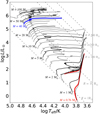 |
Fig. 1 Hertzsprung–Russell diagram of a sample of stars at metallicity Z = 4.1 × 10⁻⁵ interpolated by SEVN from the MIST stellar tracks. The blue and red lines respectively show the likely progenitors of the BH and stellar companion in Gaia BH3. |
2.3 Additional models: Parameter-space exploration
To explore the parameter space for the formation of Gaia BH3- like systems, we ran an additional set of 17 simulations varying one parameter of the fiducial simulation per time and two additional sets varying the initial conditions. For the initial conditions, we used the same set of 2 × 10⁷ binary systems as for the fiducial model.
We simulated eight additional metallicities: Z = 0.0001 (model Z1E-4), Z = 0.0004 (model Z4E-4), Z = 0.0008 (model Z8E-4), Z = 0.001 (model Z1E-3), Z = 0.004 model (Z4E- 3), Z = 0.006 (model Z6E-3), Z = 0.008 (model Z8E-3), and Z = 0.01 (model Z1E-2). We also explored the effect of the supernova kick by running four different simulations in which the kicks are drawn from a Maxwellian distribution with σrms = 1 km/s (essentially no kick, model VK1), 50 km/s (VK50), 100 km/s (VK100), and 265 km/s (VK265). In these models, the kick is not re-scaled for the ejected mass and the mass of the compact remnant. We also tested the importance of the common-envelope phase by running two simulations varying the common envelope efficiency (α = 3, model CEα3, and α = 5, model CEα5) and two additional simulations varying the binding energy formalism (model CEλXL10 using the fitting equations by Xu & Li 2010 and model CEλK21 using the fitting equations by Klencki et al. 20215). Furthermore, we ran an additional model (RLOp) in which we allowed the system to start a Roche- lobe overflow in an eccentric orbit if the condition of Roche-lobe overflow is satisfied at the periastron, that is, if the stellar radius is larger than RL = rperi f (q), where rperi is the periastron and f (q) is a function that depends on the binary mass ratio (Eggleton 1983).
Since Gaia BH3 is an eccentric system, we also ran an additional simulation (model ICthermal) to examine the impact of the initial eccentricity distribution. In this simulation, the initial orbital eccentricity is drawn from a thermal distribution, which favours eccentric systems, PDF(e) ∝ e (see e.g. Geller et al. 2019).
Finally, to assess the uncertainties due to the initial condition sampling, we drew an additional set of 1.8 × 10⁸ binaries and simulated their evolution using the same setup as the fiducial simulation. We combined the results of the additional simulations with those from the fiducial simulation, and labeled the final combined dataset as ‘fiducial2E8’. The total mass evolved in this case is Msim = 4.2 × 10⁹ M⊙, corresponding to a total population mass of Mtot = 1.4 × 10¹⁰ M⊙ (see Sect. 2.2). The results of the simulations are publicly available in Zenodo.
3 Results
Figure 2 shows the properties of the BH-star systems in the fiducial model. We considered all the simulation outputs in which a binary system is composed of a BH and a giant star, that is, a star that left the main sequence and has not started the core helium burning phase yet. We imposed the additional condition that the system is not undergoing a common-envelope or Roche-lobe overflow episode. The colour map of Fig. 2 represents the time spent by all the systems in such a configuration, which is a proxy of the likelihood of observing a given system.
Binaries hosting a BH and a massive companion are, in general, more common in the simulations, but the short lifetime of the massive star makes them less likely to be observed. In contrast, BH–low-mass star binaries are rarer, but once formed, they can remain in the same configuration for several gigayears.
Gaia BH3 is located in a region of the parameter space well covered by the fiducial simulation, especially when considering binary systems older than 10 Gyr. In addition, the Gaia BH3 properties (mostly period and BH mass) cover a range in which Gaia is particularly sensitive to astrometric signals of binarity (see e.g. Penoyre et al. 2022). From Fig. 2, we can conclude that if a BH-star system is observed in an old and metal-poor population, it is not surprising to find it with the Gaia BH3 configuration. In this sense, Gaia BH3 is not an outlier, unlike Gaia BH1 and BH2 (El-Badry et al. 2023b; Rastello et al. 2023).
It is convenient to define a region of the observed parameter space to identify Gaia BH3-like systems. For the sake of simplicity and to help the comparison with previous work, we used a selection cut similar to the one used in Marín Pina et al. (2024): P ∈ [400,40 000] days, ms ∈ [0.2, 1] M⊙, mbh ∈ [25,45] M⊙, e ∈ [0.63,0.83]. The box represents about 1% of the volume of the parameter space that includes BH-star systems at ages older than 10 Gyr.
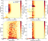 |
Fig. 2 Properties of non-interacting BH-star systems in the fiducial model. Here, we only show stars in the giant phase, that is, outside the main sequence and that have not started the core helium burning phase yet. Also, we do not show systems that undergo a Roche-lobe overflow episode. From top to bottom and from left to right: Orbital period versus companion star mass; BH mass versus companion star mass; eccentricity versus orbital period; eccentricity versus companion star mass. The colour map shows the integrated time spent by the systems in a given bin; thus, it is a proxy of the likelihood of observing a system with such properties. The map does not include information about the stellar luminosity, which is also important for detectability. We assumed a metallicity of Z = 4.1 × 10⁻⁵. The star indicates the properties of Gaia BH3, while the light blue boxes show the criteria used to select Gaia BH3-like systems. The colour maps saturate at 98% of the maximum value. |
3.1 Formation history
All the Gaia BH3-like systems in our models have the same simple formation history. Their progenitors consist of a massive star (>40 M∈) and a low-mass companion (<1 M∈). The binary components never interact through Roche-lobe overflow, so the orbital properties at BH formation are almost the same as their initial ones. The final properties of the BH-star system are thus determined by the binary phase at the moment of the supernova explosion, the amount of mass lost during the evolution, and the BH natal kick.
In our fiducial model, the initial BH progenitor mass is about 40–50 M∈, and the ejected mass at BH formation is 10–20 M∈. The mild BH natal kick (<10 km/s) cannot drastically change the binary orbital parameters. As a consequence, a large majority of BH progenitors originated with orbital properties very similar to Gaia BH3, namely, a period between 103 and 104 days and an eccentricity in the range 0.6–0.9. The system more similar to Gaia BH3 has an initial period of about 1500 days, an eccentricity of 0.65, a stellar mass of 0.83 M⊙, and an initial BH progenitor mass of 41 M⊙ . We found a sub-population (<10% of the total) that produces Gaia BH3-like systems starting from almost circular orbits (e < 0.2) and lower initial periods (<103 days). For these systems, the final orbital properties are determined by the high value of the BH natal kick. A few systems (≈3%) have very massive BH progenitors of about 120 M⊙ that produce BHs with a mass of ∼30 M⊙ because of mass loss during pulsational pair instability (Heger & Woosley 2002; Belczynski et al. 2016; Woosley 2017, 2019; Farmer et al. 2019; Costa et al. 2021; Tanikawa et al. 2021).
In all of our models, the progenitors of Gaia BH3 do not undergo any (stable or unstable) mass transfer episode. Therefore, there are no differences among the models CEα3, CEα5, CEλXL10, and CEλK21. Also, we found only a mild decrease in the number of Gaia BH3-like systems for the model RLOp, which indicates that including or not including the possibility to trigger a stable mass transfer at periastron is not important for the production of such binary systems. We found the same progenitors in the case of the kick model VK1, which serves as confirmation that in the fiducial model, the implemented kick model produces very low kicks for the case of Gaia BH3-like progenitors.
Models with higher kick velocities show significant differences in the initial orbital properties. The BH natal kicks in models VK50 and VK100 are able to wash out any correlation between the initial and final period and eccentricity. The Gaia BH3-like progenitors have initial periods and eccentricities almost uniformly distributed in the range 100–4000 days and 0–0.8, respectively. At very high velocities (model VK265), the formation of Gaia BH3-like binaries is strongly suppressed. Most systems break during BH formation, and just a few of them (four out of the 20 million simulated binaries) had a lucky configuration of binary phase and/or velocity kick that let them survive the supernova event.
We found a trend with metallicity for the initial orbital period, eccentricity, and BH progenitor mass. From low metal- licity (model Z1E-4) to intermediate-high metallicity (model Z1E-2), the lower limit of the initial period moves toward higher values (P > 1000 days for model Z1E-2), while the sub-populations with initial low eccentricity (e < 0.6) tend to disappear. As for the BH progenitor mass, the range of values widens with increasing metallicity, up to initial masses of 100 M⊙ . This is due to the non-monotonic trend of the initial BH mass relation of the MIST tracks used in this work when paired with the rapid and delayed supernova models by Fryer et al. (2012). When assuming initial masses lower than 60 M⊙, the combination of the Fryer et al. (2012) supernova models and the MIST tracks produces BHs more massive than 25 and 30 M⊙ up to a metallicity Z = 0.02 and 0.01, respectively. When relaxing the limit on the initial masses, BHs more massive than 30 M⊙ are excluded only for Z > 0.02.
Mass transfer through stellar winds is negligible (<10−9 M∈) in all of the simulated Gaia BH3-like objects. At BH formation, a typical Gaia BH3 progenitor hosts a low-mass star with stellar radius R։ < 1 R⊙ at a distance from the supernova explosion of Dsn = 1000–4000 R⊙ . Considering a total ejected mass of Mej = 10 M⊙ , the amount of mass deposited into the low-mass companion is  . As discussed by El-Badry (2024), this amount of pollution is hardly detectable in the spectral lines. In addition, the MIST models predict that a ~0.8 M⊙ star loses 10−2–10−3 M⊙ from the main-sequence to the red giant phase, likely removing all the material deposited from the supernova into the star external layer. In conclusion, we do not expect any peculiar chemical signature in the Gaia BH3 star if it formed through the isolated channel. This is consistent with the observations (Gaia Collaboration 2024).
3.2 Bayesian sampling
The SEVN simulations indicate that the region of Gaia BH3 in the observed parameter space (P, e, mBH , mms) tends to be populated by systems in which the binary components never interact. Therefore, the final binary properties are determined by the initial binary parameters and the details of the BH formation only. In order to focus on Gaia BH3 progenitors independently of the chosen selection cut, we implemented a simple Bayesian sampling technique in which we sample the posteriors of the binary initial conditions. We assume the likelihood is a multivariate normal distribution centred on the Gaia BH3 values and with the standard deviations equal to the reported errors (which we assumed to be independent).
For the parameter priors, we used:
a uniform distribution for the mean anomaly (between 0 and 2π) at the moment of the BH formation,
a uniform distribution for the mass of the BH progenitor between 20 and 100 M⊙,
a uniform distribution for eccentricity between 0 and 1,
a log-uniform distribution for the period between 10 and 106 days,
a normal distribution for the three spherical components of the velocity kick, corresponding to a Maxwellian distribution of the velocity module.
For the velocity distribution, we tested five different values of the one-dimensional root-mean-square velocity for the Maxwellian distribution (1,10,50,100,256 km/s). We also excluded the interacting binary systems by setting the prior to be equal to zero when the maximum radius of the BH progenitor is larger than either the separation at periastron or the Roche-lobe radius at periastron (see Sect. 2). To estimate the final properties of the binary, we used the formalism in the appendix of Hurley et al. (2002), and we estimated the maximum radius and the final mass of the BH progenitor by using SEVN. The posteriors were sampled using the Monte Carlo Markov chain (MCMC) ensemble sampler available in the ‘emcee’ python package (Foreman- Mackey et al. 2013). This method is similar to the grid search presented by El-Badry (2024), but our method is tailored to exactly reproducing the observed properties of Gaia BH3. Since we included the reduction of the parameter space due to stellar interactions directly in the priors, the posteriors do not need to be corrected a posteriori.
We show the posterior samples in Fig. 3. Overall, they are consistent with what was obtained from the SEVN simulations for the wider space of the selection cut assumed in Sect. 3.1. Assuming low kick velocities, the Gaia BH3 progenitor is very likely to have originated from a wide and eccentric binary (P ≈ 3500 days, e ~ 0.75). The smaller peak at around 103 days and e ~ 0.4 is due to systems that form the BH at periastron, where it is more favourable to produce large final eccentricities due to the impact of mass loss during the supernova explosion. Larger kicks widen the range of initial periods and eccentricities, with most of the initial periods being around 500–600 days. The period distribution is sharply cut below 300 days because the objects are tight enough to interact. It is possible to form a Gaia BH3 system with initial kicks up to 200 km/s. For higher values, the kick is larger than the escape velocity at periastron in the whole range of periods that are consistent with a non-interacting binary.
Independent of the explored parameters, a clear picture emerged. In the presence of low supernova kicks (<10 km/s), Gaίa BH3-like systems form from non-interacting binary progenitors preferentially in a wide (500 < P/days < 2 × 10⁴) and eccentric configuration. Alternatively, on the off chance that the binary survives to higher supernova kicks, systems with Gaia BH3 properties can form preferentially from tighter (P/days ~ 500) systems almost independently of their initial eccentricity if e < 0.7. For this reason, the initial properties of the binary can play a key role in setting the formation efficiency of Gaia BH3-like systems. Indeed, the model with a higher initial eccentricity (ICthermal) produces two to three times more Gaia BH3-like systems compared to our fiducial run (Table 1).
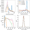 |
Fig. 3 Distribution of the initial conditions of the binaries that reproduce the Gaia BH3 properties after BH formation. From top left to bottom right, the panels show the initial binary period, initial eccentricity, the module of the BH natal kick velocity, and the initial mass of the BH progenitor. We show the distributions obtained assuming different Maxwellian-distribution priors for the kick velocity: σv = 1 km/s (blue thick solid line), σv = 10 km/s (orange thick dashed line), σv = 50 km/s (green dotted line), σv = 100 km/s (red thin solid line), σv = 256 km/s (violet thin dashed line). |
3.3 Halo population
In the explored models, Gaia BH3-like systems represent one of the standard outcomes of binary evolution. Next, we investigated how common Gaia BH3-like systems and BH-star binaries are in the Galactic halo environment, which is characterised by low metallicity and old ages. We also assumed t > 10 Gyr. First, we estimated the formation efficiency, defined as the ratio of the number of objects to the total simulated mass. We corrected the total mass in the initial conditions for the incomplete mass sampling of the primary, and we assumed an initial binary fraction of one for the sake of simplicity. Table 1 reports the formation efficiency of all the systems in the Gaia BH3 selection box (Fig. 2) as well as of those systems that are in the selection box and in the BH-star configuration after 10 Gyr.
In the fiducial model, the population of Gaia BH3-like objects accounts for about 2–3% of the whole population at t > 10 Gyr. This number is consistent with the volume fraction sampled by the selection box. Models with higher kicks significantly suppress the formation of both Gaia BH3-like and BH-star systems, while a higher metallicity increases their formation efficiency up to a factor of two. Given the formation history of Gaia BH3-like objects, the efficiency is not affected by the choice of the common-envelope ejection efficiency and binding energy. However, larger values of the common envelope efficiency parameter α slightly increase the formation efficiency of the whole BH-star systems, resulting in a lower fraction of Gaia BH3-like systems.
Even if the Galactic stellar halo is the least massive component of our Galaxy, the most recent estimates revise its mass from a few 108 M⊙ (see, e.g., Bell et al. 2008) up to 0.7–1.2 × 10⁹ M⊙ (Deason et al. 2019; Lane et al. 2023). Combining the total halo mass with the formation efficiencies in Table 1, we predict the number of BH stars in the halo to be in the range of ≈1000–4000. Among these systems, about 20–120 fall in the Gaia BH3 selection cut used in this work (Fig. 2). The Galactic stellar halo is a diffuse component extended up to 100 kpc with a steep density profile (ρ ∝ r–γ, with 2 < γ < 5; see, e.g., Medina et al. 2024; Iorio et al. 2018 and references therein).
Deason et al. (2019) report a local density profile at the Sun location of ρh,⊙ ≈ 8 × 10⁴ M⊙/kpc3. Multiplying this density by the formation efficiencies of the old BH-star binaries, we obtained a local density of nBHStar = ηBHStar ρh,⊙ ranging from 0.1 to 0.3 kpc–3. The values correspond to an expected number of objects between 0.13 and 0.27 at the distance of Gaia BH3 (≈0.6 kpc). At face value, we do not expect any BH-star binary system from the halo in the solar neighbourhood. However, we can account for the statistical noise by assuming that the number of systems follows a Poissonian distribution with the rate λBHStar ranging between 0.13 and 0.27. In this case, the probability to observe at least one object is between 12% and 25%. By simply using the formation efficiency for the old systems in the Gaia BH3 selection box (Fig. 2), we obtained a Poisson rate between 0.003 and 0.006, corresponding to a probability of observing at least one Gaia BH3-like system of 0.3–0.6%. Although these numbers correspond to the very low probability tail of the distribution, they cannot be rejected at the 3σ level. However, a single future detection of another Gaia BH3-like binary system in the Galactic halo within the solar neighbourhood would be enough to significantly rule out the isolated formation channel, according to the models presented in this work. However, this will also represent a challenge for the alternative dynamical formation channel (see Sect. 4.4).
Formation efficiency ( ) for Gaia BH3-like and BH-star systems obtained from different simulation models.
3.4 Populations in the stellar clusters and cold structures
Balbinot et al. (2024) show that Gaia BH3 is associated with the ED-2 stellar stream. The presence of Gaia BH3-like systems in star clusters and kinematically cold structures, such as a stellar stream, pose additional constraints on the natal kick velocity in the binary centre of mass, vsys. In fact, if the kick velocity is significantly larger than the typical velocity dispersion of the host cluster or stream, the BH will escape from the system and join the field population in the Milky Way. The escape velocity from globular clusters ranges from ~ 10 km s–1 km to ~50 km s–1 (Gnedin et al. 2002). Almost all (> 90%) the Gaia BH-3 systems in our simulations have vsys < 50 km s–1, except for models VK50, VK100, and VK265 (Fig. 3).
Focusing on the low-velocity tail of the kick distribution, Table 1 reports the formation efficiency of Gaia BH3-like systems when we apply the additional selection cut of vsys < 10 km s–1 (typical velocity dispersion of globular clusters) and vsys < 1 km s–1 (drift velocity of the ED-2 components with respect to the progenitor cluster; Marín Pina et al. 2024). For most of our models, the formation efficiency decreases by ≤20–30%. Although the effect is not negligible, the formation efficiency decrease is not significant enough to rule out the isolated formation channel for Gaia BH3-like systems at a 3σ level.
4 Discussion
4.1 Stellar evolution models
Uncertainties about massive star evolution have an important impact on our results. For instance, differences in the maximum radius of the BH progenitor are crucial to selecting which objects interact during binary evolution.
El-Badry (2024) explored the main uncertainties about stellar evolution models, concluding that most models predict that the progenitor of Gaia BH3 reached radii up to 1000 R⊙. Such stars cannot avoid interaction before BH formation. For this reason, El-Badry (2024) conclude that dynamical interactions in a star cluster represent the only possible formation channel for Gaia BH3, unless the radius of the BH progenitor did not exceed ≈700 R⊙. In our stellar evolution models based on the MIST tracks (Choi et al. 2016), the BH progenitor reaches a maximum radius of ≲200–300 R⊙ for Z < 0.0002 (Fig. 1). We find similar results for the PARSEC stellar tracks (Bressan et al. 2012; Chen et al. 2015; Costa et al. 2021; Nguyen et al. 2022) available in SEVN (Iorio et al. 2023). While a detailed analysis of the differences in stellar evolution models is beyond the scope of this paper (see, e.g., Agrawal et al. 2020, 2022a,b; Klencki et al. 2020; Gilkis et al. 2021), it is still crucial to note their significant impact on the interpretation of Gaia BH3 and other BH-star systems.
4.2 Initial eccentricity and stellar tides
In all the simulations assuming our fiducial kick model (Giacobbo & Mapelli 2020), Gaia BH3-like systems form preferentially from binary systems with an initial eccentric orbit (e > 0.6). Therefore, we expect that initial distributions that favour eccentric orbits, such as the thermal distribution, boost the number of Gaia BH3-like systems (model ICthermal; see Table 1). In contrast, circular orbits significantly suppress the formation of such systems unless high kick models are used.
In some cases, initial circular binaries are justified by the effect of tides. The SEVN simulations used in this work implement the tides following the formalism by Hurley et al. (2002) (see also Iorio et al. 2023) and show that for Gaia BH3-like systems, tides are extremely inefficient. The tidal efficiency is at its maximum after the main-sequence phase of the BH progenitor, when the star expands and develops a convective envelope. Assuming that the dominant tidal dissipation mechanism is due to convective motions in the envelope (Zahn 1977; Hurley et al. 2002) and considering the MIST models at Z = 4.1 × 10⁻⁵ (Fig. 1), we estimated a circularisation timescale due to tides of τcirc ≃ 1025–1038 Gyr. This timescale is orders of magnitude longer than the lifetime of the binary system and especially longer than the post main-sequence phase, when tides are more efficient.
4.3 Systematic uncertainties
Table 1 shows that the formation efficiency of BH-star systems drops significantly for models with high supernova kicks. In the models VK100 and VK265, we can exclude the hypothesis that the observation of Gaia BH3 is consistent with the isolated channel at a high level of significance (>3σ). Estimates of BH kicks rely on a few tracers (e.g. X-ray binaries) and are subject to many uncertainties and systematics (see, e.g., Andrews & Kalogera 2022; Atri et al. 2019; Shenar et al. 2022a). The association of Gaia BH3 with a stellar stream (Balbinot et al. 2024) indicates that the binary system did not experience a kick much higher than the typical escape velocity from a star cluster (< 10 km/s) at the time of BH formation (Sect. 3.4).
In our analysis, we did not consider binaries with companion stars less massive than 0.71 M⊙. As discussed by El-Badry (2024), such a population can represent a significant portion of the stellar companions of Gaia BH3-like systems. To assess the relevance of this population on the estimate of the formation efficiency, we generated new initial conditions, as done in Sect. 2.1, but we assumed an extended mass ratio range from 0.08 M⊙/m1 to 1. We find that the percentage of binaries hosting a BH progenitor and a secondary star less massive than 0.71 M⊙ is 40% of similar binaries with a secondary in the mass range 0.71-1.0 M⊙. Therefore, we expect an overall increase in the formation efficiency by about 40% with respect to the value reported in Table 1. This factor is balanced by the commonly assumed binary fraction in stellar populations (40-60%; see, e.g., Moe & Di Stefano 2017).
Many population synthesis studies on BH-star binaries are based on stellar evolution models by Pols et al. (1998) (see, e.g., Breivik et al. 2017; Shao & Li 2019; Olejak et al. 2020; Chawla et al. 2022; Shikauchi et al. 2023; Di Carlo et al. 2024). In general, the stars in these tracks tend to expand to larger radii compared to the MIST models. Most of these works focus on the Galactic population, of which the stellar halo is a negligible component. Hence a direct comparison is not straightforward. We note that the properties of the few metal-poor stars reported by Chawla et al. (2022) and the halo population discussed by Olejak et al. (2020) seem to be qualitatively consistent with the distribution of the BH-star systems found in our simulations in terms of period and companion mass.
Di Carlo et al. (2024) report a BH star formation efficiency for the isolated channel at least one order of magnitude lower than what we found in our simulations. Moreover, these authors claim that any BH-star system with an eccentricity larger than 0.5 and a BH mass larger than 30 Mø are exclusively associated with the dynamical formation channel. The origin of this discrepancy is twofold. First, their sample is dominated by the metal-rich population of the Milky Way disc. Secondly, their stellar and binary evolution models are significantly different from the ones adopted in this work. In particular, Di Carlo et al. (2024) used stellar tracks by Pols et al. (1998) and a different supernova and natal kick model.
The number of binaries simulated in our models correspond to a stellar population with a total mass of ~109 M⊙. This mass is representative of the old and metal-poor Galactic stellar halo (Deason et al. 2019). However, a single halo realisation suffers from stochastic fluctuations. The model fiducial2E8, in which we simulated 2 × 10⁸ binaries, indicates that our fiducial model slightly underestimates the number of Gaia BH3-like binaries (Table 1). However, by dividing the initial conditions of fiducial2E8 (Sect. 2.3) into sub-samples of 2 × 10⁷ binaries, we are able to confirm that the errors quoted in Table 1 realistically capture the uncertainties.
4.4 Alternative formation channel
Gaia BH3 is associated with the ED-2 stream (Balbinot et al. 2024). Therefore, it possibly spent a part of its life in a dynamical environment. The variety of interactions in dynamical environments has two competitive effects. On the one hand, they can pair BHs and stars or create binary systems with orbital properties (e.g. high eccentricities) that boost the production of Gaia BH3-like binaries. On the other hand, dynamical interactions could destroy original and newly formed BH-star systems, especially if their orbit is wide and the companion is a low-mass star.
The other two BH-star systems retrieved from Gaia data (BH1, El-Badry et al. 2023b; Chakrabarti et al. 2023, and BH2, El-Badry et al. 2023a) are difficult to reconcile with isolated binary evolution models (El-Badry et al. 2023a). However, they are more easily formed in star clusters (Rastello et al. 2023; Di Carlo et al. 2024; Tanikawa et al. 2024, but see Kotko et al. 2024).
Marín Pina et al. (2024) show that BH-star systems dynamically form in an efficient way in globular clusters with mass 105–106 M⊙. They estimated a formation efficiency of  by considering all the BH-star systems formed in their Monte Carlo simulations (both escaped or retained in the cluster). Di Carlo et al. (2024) estimate a formation efficiency of
  by considering star clusters in the mass range 103 – 3 × 10⁴ M⊙; Rastello et al. (2023) show that the formation efficiency rises up to
  for low-mass clusters (≈ 102– 103 M⊙) at high metallicity (Z = 0.02). Assuming a mass of the ED-2 cluster progenitor in the range ~103–104 (Balbinot et al. 2024), the dynamical channel is one to two orders of magnitude more efficient than the isolated channel presented in this work. However, when considering the mass of the halo (Deason et al. 2019) and the cluster radial profile (e.g. Gieles & Gnedin 2023), the difference on the expected formation efficiency of BH-star systems in the solar neighbourhood reduces to a factor of three to ten between the isolated and star cluster scenario.
When focusing specifically on Gaia BH3-like systems, Marín Pina et al. (2024) find that only 0.6% of their BH-star systems (nine out of 1435) fall within the same selection box used in our work (Fig. 2), and only two of them (0.1%) are candidates to be within an ED2-like stream at the present time (i.e. they experience a late ejection or are still in the cluster at the end of the simulation; Marín Pina, private communication). This fraction is a factor of two to ten smaller than what we found in our fiducial model (see Table 1) when considering only old Gaia BH3-like systems that received a low natal kick (Table 1). Therefore, the ratio between the dynamical to isolated formation efficiency ranges from 0.6 (isolated channel slightly favoured) to 90 (dynamical channel strongly favoured). Considering the model with the higher Gaia BH3-like formation efficiency (ICthermal; see Table 1), the ratio ranges from 0.1 (isolated formation channel favoured) to 20 (dynamical formation channel favoured). Marín Pina et al. (2024) selected Gaia BH-3-like systems using a wider eccentricity range: from 0.5 to 0.9. With this selection criterion, the number of Gaia BH-3-like systems approximately doubles, yet the ratio between the isolated and dynamical channels remains unchanged. Taken at face value, these numbers seem to indicate that although the dynamical channel has an overall higher likelihood to form Gaia BH3, we cannot rule out the possibility that the system is compatible with a primordial binary star that escaped from the ED2 cluster.
A more quantitative comparison and model selection would require a detailed analysis of systematics, including stellar evolution models, selection effects, channel definitions, and halo population models (see e.g. Di Carlo et al. 2024). Additionally, the use of robust statistical tools is essential, as highlighted by studies such as Mould et al. (2023). However, these aspects are beyond the scope of this paper.
5 Summary
We have explored the formation of Gaia BH3 (Gaia Collaboration 2024), a non-interacting binary system composed of a massive BH (≈30 M⊙) and a low-mass giant star (≈0.8 M⊙), by means of population synthesis simulations. We have exploited the flexibility of our code SEVN (Iorio et al. 2023) to perform the first population study of BH-star systems using the MIST stellar models (Choi et al. 2016). We explored the parameter space by considering nine different metallicities, four different supernova kick models, five models for the common envelope, two models for the onset of Roche-lobe overflow, and three different sets of initial conditions. We also implemented a Bayesian sampling analysis to study the distribution of initial conditions that reproduce the observed properties of Gaia BH3 exactly. The main takeaways of our analysis are as follows:
Systems such as Gaia BH3 represent a common product of isolated binary evolution at low metallicity (Z < 0.01). They form preferentially from a massive star (40–60 M⊙) in an initially wide (P > 103 days) and eccentric (e > 0.6) orbit with a low-mass companion. The progenitor binary system never underwent Roche-lobe overflow during its life;
Our fiducial natal kick model (Giacobbo & Mapelli 2020) produces low natal kicks for Gaia BH3-like systems, leaving the initial orbital properties of the binary almost unchanged. The formation of Gaia BH3 is possible up to kicks as high as 220 km/s, but such high kicks require fine-tuning for the properties at BH formation, reducing the overall formation efficiency by about one order of magnitude, and they are not compatible with the association with a cold stellar stream;
Focusing on systems older than 10 Gyr, we find a formation efficiency of
 for BH-star binaries in general and
  for Gaia BH3-like systems;
Considering the Galactic stellar halo model by Deason et al. (2019), we expected up to ≈ 4000 BH-star systems born in the stellar halo from isolated evolution. About 20–120 of them are Gaia BH3-like systems in terms of mass and orbital properties.
Overall, Gaia BH3 is compatible with a primordial, metal-poor binary system that never evolved via Roche-lobe overflow and experienced a long, 'boring' life. Given its association with the ED-2 stream, Gaia BH3 was born in a stellar cluster but is compatible with a primordial binary star that escaped from its parent cluster without experiencing significant dynamical interactions. Unlike Gaia BH1 and BH2, its orbital properties are easy to explain with current stellar and binary evolution models. However, uncertainties about massive star evolution (e.g. maximum stellar radius of the BH progenitor) and natal kicks substantially affect our final results. Future detections of dormant BHs are thus crucial to set constraints on massive star and natal kick models.
Data availability
Our initial conditions and parameter files are publicly available at https://zenodo.org/records/11617742. The sample of BH-star systems produced in the simulations can be downloaded from https://zenodo.org/records/11992265, https://zenodo.org/records/12188369, and https://zenodo.org/records/12189734.
Acknowledgements
The authors thank the anonymous referee for their suggestions that helped us to improve the manuscript. We thank Daniel Marín Pina and Pasquale Panuzzo for useful comments, and Jakub Klencki for his contribution in revising the implementation of the Klencki2l binding energy prescriptions in SEVN. GI acknowledges financial support under the National Recovery and Resilience Plan (NRRP), Mission 4, Component 2, Investment 1.4, - Call for tender No. 3138 of 18/12/2021 of Italian Ministry of University and Research funded by the European Union - NextGenerationEU. MM, ST, MD, StR, GE, EK, EL and MPV acknowledge financial support from the European Research Council for the ERC Consolidator grant DEMOBLACK, under contract no. 770017. MM, ST, StR and MPV also acknowledge financial support from the German Excellence Strategy via the Heidelberg Cluster of Excellence (EXC 2181 – 390900948) STRUCTURES. MD also acknowledges financial support from Cariparo foundation under grant 55440. AAT acknowledges support from the European Union’s Horizon 2020 and Horizon Europe research and innovation programs under the Marie Skłodowska-Curie grant agreements no. 847523 and 101103134. SaR acknowledges support from the Beatriu de Pinós postdoctoral program under the Ministry of Research and Universities of the Government of Catalonia (Grant Reference No. 2021 BP 00213). MAS acknowledges funding from the European Union’s Horizon 2020 research and innovation programme under the Marie Skłodowska-Curie grant agreement No. 101025436 (project GRACE-BH, PI: Manuel Arca Sedda). MAS acknowledge financial support from the MERAC Foundation. Part of this work was supported by the German Deutsche Forschungsgemeίnschaft, DFG project number Ts 17/2-1. Numerical calculations have been made possible through a CINECA-INFN (TEONGRAV) agreement, providing access to resources on Leonardo at CINECA. This work has made use of data from the European Space Agency (ESA) mission Gaia (https://www.cosmos.esa.int/gaia), processed by the Gaia Data Processing and Analysis Consortium (DPAC, https://www.cosmos.esa.int/web/gaia/dpac/consortium). Funding for the DPAC has been provided by national institutions, in particular the institutions participating in the Gaia Multilateral Agreement.
References
- Abbott, B. P., Abbott, R., Abbott, T. D., et al. 2016a, Phys. Rev. Lett., 116, 061102 [Google Scholar]
- Abbott, B. P., Abbott, R., Abbott, T. D., et al. 2016b, Phys. Rev. Lett., 116, 241102 [NASA ADS] [CrossRef] [Google Scholar]
- Abbott, R., Abbott, T. D., Abraham, S., et al. 2021, Phys. Rev. X, 11, 021053 [Google Scholar]
- Abbott, R., Abbott, T. D., Acernese, F., et al. 2023, Phys. Rev. X, 13, 041039 [Google Scholar]
- Abbott, R., Abbott, T. D., Acernese, F., et al. 2024, Phys. Rev. D, 109, 022001 [NASA ADS] [CrossRef] [Google Scholar]
- Agrawal, P., Hurley, J., Stevenson, S., Szécsi, D., & Flynn, C. 2020, MNRAS, 497, 4549 [NASA ADS] [CrossRef] [Google Scholar]
- Agrawal, P., Stevenson, S., Szécsi, D., & Hurley, J. 2022a, A&A, 668, A90 [NASA ADS] [CrossRef] [EDP Sciences] [Google Scholar]
- Agrawal, P., Szécsi, D., Stevenson, S., Eldridge, J. J., & Hurley, J. 2022b, MNRAS, 512, 5717 [NASA ADS] [CrossRef] [Google Scholar]
- Andrews, J. J., & Kalogera, V. 2022, ApJ, 930, 159 [NASA ADS] [CrossRef] [Google Scholar]
- Atri, P., Miller-Jones, J. C. A., Bahramian, A., et al. 2019, MNRAS, 489, 3116 [NASA ADS] [CrossRef] [Google Scholar]
- Balbinot, E., Dodd, E., Matsuno, T., et al. 2024, A&A, 687, L3 [NASA ADS] [CrossRef] [EDP Sciences] [Google Scholar]
- Belczynski, K., Bulik, T., Fryer, C. L., et al. 2010, ApJ, 714, 1217 [NASA ADS] [CrossRef] [Google Scholar]
- Belczynski, K., Heger, A., Gladysz, W., et al. 2016, A&A, 594, A97 [NASA ADS] [CrossRef] [EDP Sciences] [Google Scholar]
- Bell, E. F., Zucker, D. B., Belokurov, V., et al. 2008, ApJ, 680, 295 [Google Scholar]
- Breivik, K., Chatterjee, S., & Larson, S. L. 2017, ApJ, 850, L13 [CrossRef] [Google Scholar]
- Bressan, A., Marigo, P., Girardi, L., et al. 2012, MNRAS, 427, 127 [NASA ADS] [CrossRef] [Google Scholar]
- Casares, J., Negueruela, I., Ribó, M., et al. 2014, Nature, 505, 378 [Google Scholar]
- Chakrabarti, S., Simon, J. D., Craig, P. A., et al. 2023, AJ, 166, 6 [NASA ADS] [CrossRef] [Google Scholar]
- Chawla, C., Chatterjee, S., Breivik, K., et al. 2022, ApJ, 931, 107 [NASA ADS] [CrossRef] [Google Scholar]
- Chen, Y., Bressan, A., Girardi, L., et al. 2015, MNRAS, 452, 1068 [Google Scholar]
- Choi, J., Dotter, A., Conroy, C., et al. 2016, ApJ, 823, 102 [Google Scholar]
- Claeys, J. S. W., Pols, O. R., Izzard, R. G., Vink, J., & Verbunt, F. W. M. 2014, A&A, 563, A83 [NASA ADS] [CrossRef] [EDP Sciences] [Google Scholar]
- Costa, G., Bressan, A., Mapelli, M., et al. 2021, MNRAS, 501, 4514 [NASA ADS] [CrossRef] [Google Scholar]
- Costa, G., Mapelli, M., Iorio, G., et al. 2023, MNRAS, 525, 2891 [NASA ADS] [CrossRef] [Google Scholar]
- Deason, A. J., Belokurov, V., & Sanders, J. L. 2019, MNRAS, 490, 3426 [NASA ADS] [CrossRef] [Google Scholar]
- Di Carlo, U. N., Agrawal, P., Rodriguez, C. L., & Breivik, K. 2024, ApJ, 965, 22 [CrossRef] [Google Scholar]
- Eggleton, P. P. 1983, ApJ, 268, 368 [Google Scholar]
- El-Badry, K. 2024, Open J. Astrophys., 7, 38 [NASA ADS] [Google Scholar]
- El-Badry, K., Rix, H.-W., Cendes, Y., et al. 2023a, MNRAS, 521, 4323 [NASA ADS] [CrossRef] [Google Scholar]
- El-Badry, K., Rix, H.-W., Quataert, E., et al. 2023b, MNRAS, 518, 1057 [Google Scholar]
- Farmer, R., Renzo, M., de Mink, S. E., Marchant, P., & Justham, S. 2019, ApJ, 887, 53 [Google Scholar]
- Foreman-Mackey, D., Hogg, D. W., Lang, D., & Goodman, J. 2013, PASP, 125, 306 [Google Scholar]
- Fryer, C. L., Belczynski, K., Wiktorowicz, G., et al. 2012, ApJ, 749, 91 [Google Scholar]
- Gaia Collaboration (Vallenari, A., et al.) 2023, A&A, 674, A1 [NASA ADS] [CrossRef] [EDP Sciences] [Google Scholar]
- Gaia Collaboration (Panuzzo, P., et al.) 2024, A&A, 686, L2 [NASA ADS] [CrossRef] [EDP Sciences] [Google Scholar]
- Geller, A. M., Leigh, N. W. C., Giersz, M., Kremer, K., & Rasio, F. A. 2019, ApJ, 872, 165 [NASA ADS] [CrossRef] [Google Scholar]
- Generozov, A., & Perets, H. B. 2024, ApJ, 964, 83 [NASA ADS] [CrossRef] [Google Scholar]
- Giacobbo, N., & Mapelli, M. 2020, ApJ, 891, 141 [NASA ADS] [CrossRef] [Google Scholar]
- Gieles, M., & Gnedin, O. Y. 2023, MNRAS, 522, 5340 [NASA ADS] [CrossRef] [Google Scholar]
- Giesers, B., Dreizler, S., Husser, T.-O., et al. 2018, MNRAS, 475, L15 [NASA ADS] [CrossRef] [Google Scholar]
- Giesers, B., Kamann, S., Dreizler, S., et al. 2019, A&A, 632, A3 [NASA ADS] [CrossRef] [EDP Sciences] [Google Scholar]
- Gilkis, A., Shenar, T., Ramachandran, V., et al. 2021, MNRAS, 503, 1884 [NASA ADS] [CrossRef] [Google Scholar]
- Gnedin, O. Y., Zhao, H., Pringle, J. E., et al. 2002, ApJ, 568, L23 [Google Scholar]
- Guseinov, O. K., & Zel’dovich, Y. B. 1966, Soviet Ast., 10, 251 [Google Scholar]
- Heger, A., & Woosley, S. E. 2002, ApJ, 567, 532 [Google Scholar]
- Hobbs, G., Lorimer, D. R., Lyne, A. G., & Kramer, M. 2005, MNRAS, 360, 974 [Google Scholar]
- Hurley, J. R., Tout, C. A., & Pols, O. R. 2002, MNRAS, 329, 897 [Google Scholar]
- Hut, P. 1981, A&A, 99, 126 [NASA ADS] [Google Scholar]
- Iorio, G., Belokurov, V., Erkal, D., et al. 2018, MNRAS, 474, 2142 [NASA ADS] [CrossRef] [Google Scholar]
- Iorio, G., Mapelli, M., Costa, G., et al. 2023, MNRAS, 524, 426 [NASA ADS] [CrossRef] [Google Scholar]
- Ivanova, N., Justham, S., Chen, X., et al. 2013, A&A Rev., 21, 59 [NASA ADS] [CrossRef] [Google Scholar]
- Klencki, J., Nelemans, G., Istrate, A. G., & Pols, O. 2020, A&A, 638, A55 [NASA ADS] [CrossRef] [EDP Sciences] [Google Scholar]
- Klencki, J., Nelemans, G., Istrate, A. G., & Chruslinska, M. 2021, A&A, 645, A54 [EDP Sciences] [Google Scholar]
- Kotko, I., Banerjee, S., & Belczynski, K. 2024, MNRAS, submitted [arXiv:2403.13579] [Google Scholar]
- Kroupa, P. 2001, MNRAS, 322, 231 [NASA ADS] [CrossRef] [Google Scholar]
- Lane, J. M. M., Bovy, J., & Mackereth, J. T. 2023, MNRAS, 526, 1209 [NASA ADS] [CrossRef] [Google Scholar]
- Lennon, D. J., Dufton, P. L., Villaseñor, J. I., et al. 2022, A&A, 665, A180 [NASA ADS] [CrossRef] [EDP Sciences] [Google Scholar]
- Mahy, L., Sana, H., Shenar, T., et al. 2022, A&A, 664, A159 [NASA ADS] [CrossRef] [EDP Sciences] [Google Scholar]
- Mapelli, M., Colpi, M., & Zampieri, L. 2009, MNRAS, 395, L71 [NASA ADS] [CrossRef] [Google Scholar]
- Mapelli, M., Ripamonti, E., Zampieri, L., Colpi, M., & Bressan, A. 2010, MNRAS, 408, 234 [NASA ADS] [CrossRef] [Google Scholar]
- Mapelli, M., Zampieri, L., Ripamonti, E., & Bressan, A. 2013, MNRAS, 429, 2298 [NASA ADS] [CrossRef] [Google Scholar]
- Mapelli, M., Spera, M., Montanari, E., et al. 2020, ApJ, 888, 76 [NASA ADS] [CrossRef] [Google Scholar]
- Marín Pina, D., Rastello, S., Gieles, M., et al. 2024, A&A, 688, L2 [NASA ADS] [CrossRef] [EDP Sciences] [Google Scholar]
- Medina, G. E., Muñoz, R. R., Carlin, J. L., et al. 2024, MNRAS, 531, 4762 [NASA ADS] [CrossRef] [Google Scholar]
- Miller-Jones, J. C. A., Bahramian, A., Orosz, J. A., et al. 2021, Science, 371, 1046 [Google Scholar]
- Moe, M., & Di Stefano, R. 2017, ApJS, 230, 15 [Google Scholar]
- Mould, M., Gerosa, D., Dall’Amico, M., & Mapelli, M. 2023, MNRAS, 525, 3986 [NASA ADS] [CrossRef] [Google Scholar]
- Nguyen, C. T., Costa, G., Girardi, L., et al. 2022, A&A, 665, A126 [NASA ADS] [CrossRef] [EDP Sciences] [Google Scholar]
- Oëzel, F., Psaltis, D., Narayan, R., & McClintock, J. E. 2010, ApJ, 725, 1918 [CrossRef] [Google Scholar]
- Olejak, A., Belczynski, K., Bulik, T., & Sobolewska, M. 2020, A&A, 638, A94 [NASA ADS] [CrossRef] [EDP Sciences] [Google Scholar]
- Penoyre, Z., Belokurov, V., & Evans, N. W. 2022, MNRAS, 513, 2437 [NASA ADS] [CrossRef] [Google Scholar]
- Pols, O. R., Schroder, K.-P., Hurley, J. R., Tout, C. A., & Eggleton, P. P. 1998, MNRAS, 298, 525 [NASA ADS] [CrossRef] [Google Scholar]
- Rastello, S., Iorio, G., Mapelli, M., et al. 2023, MNRAS, 526, 740 [NASA ADS] [CrossRef] [Google Scholar]
- Ribó, M., Munar-Adrover, P., Paredes, J. M., et al. 2017, ApJ, 835, L33 [Google Scholar]
- Sana, H., de Mink, S. E., de Koter, A., et al. 2012, Science, 337, 444 [Google Scholar]
- Saracino, S., Kamann, S., Guarcello, M. G., et al. 2022, MNRAS, 511, 2914 [NASA ADS] [CrossRef] [Google Scholar]
- Saracino, S., Shenar, T., Kamann, S., et al. 2023, MNRAS, 521, 3162 [NASA ADS] [CrossRef] [Google Scholar]
- Sgalletta, C., Iorio, G., Mapelli, M., et al. 2023, MNRAS, 526, 2210 [NASA ADS] [CrossRef] [Google Scholar]
- Shao, Y., & Li, X.-D. 2019, ApJ, 885, 151 [NASA ADS] [CrossRef] [Google Scholar]
- Shenar, T., Sana, H., Mahy, L., et al. 2022a, Nat. Astron., 6, 1085 [NASA ADS] [CrossRef] [Google Scholar]
- Shenar, T., Sana, H., Mahy, L., et al. 2022b, A&A, 665, A148 [NASA ADS] [CrossRef] [EDP Sciences] [Google Scholar]
- Shikauchi, M., Tsuna, D., Tanikawa, A., & Kawanaka, N. 2023, ApJ, 953, 52 [NASA ADS] [CrossRef] [Google Scholar]
- Spera, M., & Mapelli, M. 2017, MNRAS, 470, 4739 [Google Scholar]
- Spera, M., Mapelli, M., & Bressan, A. 2015, MNRAS, 451, 4086 [NASA ADS] [CrossRef] [Google Scholar]
- Spera, M., Mapelli, M., Giacobbo, N., et al. 2019, MNRAS, 485, 889 [Google Scholar]
- Tanikawa, A., Susa, H., Yoshida, T., Trani, A. A., & Kinugawa, T. 2021, ApJ, 910, 30 [NASA ADS] [CrossRef] [Google Scholar]
- Tanikawa, A., Hattori, K., Kawanaka, N., et al. 2023, ApJ, 946, 79 [CrossRef] [Google Scholar]
- Tanikawa, A., Cary, S., Shikauchi, M., Wang, L., & Fujii, M. S. 2024, MNRAS, 527, 4031 [Google Scholar]
- Thompson, T. A., Kochanek, C. S., Stanek, K. Z., et al. 2019, Science, 366, 637 [NASA ADS] [CrossRef] [Google Scholar]
- Trimble, V. L., & Thorne, K. S. 1969, ApJ, 156, 1013 [Google Scholar]
- Webbink, R. F. 1984, ApJ, 277, 355 [NASA ADS] [CrossRef] [Google Scholar]
- Woosley, S. E. 2017, ApJ, 836, 244 [Google Scholar]
- Woosley, S. E. 2019, ApJ, 878, 49 [Google Scholar]
- Xu, X.-J., & Li, X.-D. 2010, ApJ, 722, 1985 [NASA ADS] [CrossRef] [Google Scholar]
- Zahn, J. P. 1977, A&A, 57, 383 [Google Scholar]
- Zampieri, L., & Roberts, T. P. 2009, MNRAS, 400, 677 [NASA ADS] [CrossRef] [Google Scholar]
- Ziosi, B. M., Mapelli, M., Branchesi, M., & Tormen, G. 2014, MNRAS, 441, 3703 [Google Scholar]
In this work, we used the SEVN version V 2.10.1 (commit a4753f11) publicly available at the GitLab repository https://gitlab.com/sevncodes/sevn
The version of the code we used to produce the tables is available at https://gitlab.com/sevncodes/trackcruncher (commit0827337).
We assumed a parent population with primary masses m1 between 0.08 Mѳ and 150 Mѳ and mass ratios in the range q ∈ [0.08 M⊙/m1,1].
In SEVN version 2.10.0, we revised the implementation of the λK21 fitting equations by Klencki et al. 2021. We corrected a bug in the code that affected the λK21 estimate for metallicities Z < 0.017 (the bug has been fixed for all the versions greater than 2.8.0). Additionally, we improved the fit for cases in which the stellar radius is less than the radius at the terminal age main sequence (TAMS) of the MESA stellar tracks used in Klencki et al. (2021) (private communication). In this radial range, the original fitting equations were extrapolated, leading to high binding energies (>1052 ergs). For additional information, we refer to the discussion in the SEVN repository: https://gitlab.com/sevncodes/sevn/-/issues/4
All Tables
Formation efficiency () for Gaia BH3-like and BH-star systems obtained from different simulation models.
All Figures
|
Fig. 1 Hertzsprung–Russell diagram of a sample of stars at metallicity Z = 4.1 × 10⁻⁵ interpolated by SEVN from the MIST stellar tracks. The blue and red lines respectively show the likely progenitors of the BH and stellar companion in Gaia BH3. |
| In the text | |
|
Fig. 2 Properties of non-interacting BH-star systems in the fiducial model. Here, we only show stars in the giant phase, that is, outside the main sequence and that have not started the core helium burning phase yet. Also, we do not show systems that undergo a Roche-lobe overflow episode. From top to bottom and from left to right: Orbital period versus companion star mass; BH mass versus companion star mass; eccentricity versus orbital period; eccentricity versus companion star mass. The colour map shows the integrated time spent by the systems in a given bin; thus, it is a proxy of the likelihood of observing a system with such properties. The map does not include information about the stellar luminosity, which is also important for detectability. We assumed a metallicity of Z = 4.1 × 10⁻⁵. The star indicates the properties of Gaia BH3, while the light blue boxes show the criteria used to select Gaia BH3-like systems. The colour maps saturate at 98% of the maximum value. |
| In the text | |
|
Fig. 3 Distribution of the initial conditions of the binaries that reproduce the Gaia BH3 properties after BH formation. From top left to bottom right, the panels show the initial binary period, initial eccentricity, the module of the BH natal kick velocity, and the initial mass of the BH progenitor. We show the distributions obtained assuming different Maxwellian-distribution priors for the kick velocity: σv = 1 km/s (blue thick solid line), σv = 10 km/s (orange thick dashed line), σv = 50 km/s (green dotted line), σv = 100 km/s (red thin solid line), σv = 256 km/s (violet thin dashed line). |
| In the text | |
Current usage metrics show cumulative count of Article Views (full-text article views including HTML views, PDF and ePub downloads, according to the available data) and Abstracts Views on Vision4Press platform.
Data correspond to usage on the plateform after 2015. The current usage metrics is available 48-96 hours after online publication and is updated daily on week days.
Initial download of the metrics may take a while.