© The Authors 2024

1 Introduction

One of the major goals of modern astrophysics is to understand how and when structures formed in the Universe. In particular, the speed at which a gaseous system, like a molecular cloud, undergoes gravitational collapse and produces stars is of great importance. Estimating the star formation rate (SFR) in various systems has been the subject of many observational studies during the last decades (e.g. Schmidt 1959; Lada et al. 2010; Kennicutt & Evans 2012; Schruba et al. 2019; Sun et al. 2023) and remains an active field of research as new telescopes such as JWST push the boundaries of extra-galactic observations and resolve star forming regions within the Milky Way with extraordinary detail. A major puzzle is the remarkably small value of the SFR, typically found to be about two orders of magnitude below the simplest estimate obtained by dividing the mass of dense gas by the freefall time of the system. This fact is generally interpreted as the consequence of support against gravitational collapse, which could be due to either magnetic fields (Shu et al. 1987) or turbulence (Zuckerman & Palmer 1974; Zuckerman & Evans 1974; Mac Low & Klessen 2004). The role of stellar feedback is also heavily emphasised, particularly through numerous numerical simulations (e.g. Kim et al. 2013; Walch & Naab 2015; Iffrig & Hennebelle 2017). In this context, the exact distinction between the role played by feedback and turbulence is partially unclear. Feedback is certainly a source of turbulence, but it also creates diverging motion that destroys star-forming clouds, limiting the star formation efficiency of these clouds.

In an attempt to understand and predict how the SFR is determined, several models have been developed, particularly during the last two decades (Krumholz & McKee 2005; Padoan & Nordlund 2011; Hennebelle & Chabrier 2011; Renaud et al. 2012). Most of these models, as presented in more detail below, rely on the idea that only gas above a certain density is undergoing collapse. Therefore, they integrate the density probability density function (PDF) above a selected density threshold that generally derives from the sonic and the Jeans length. A somewhat different approach has been followed by Hennebelle & Chabrier (2011), where it is proposed to proceed in two steps. First, the mass spectrum of self-gravitating clouds is inferred. This step entails the spatial coherence, that is the power spectrum, of the density field (more precisely, the natural logarithm of the density field). Once this step is completed, the sum over this mass spectrum divided by the freefall time provides an estimate for the SFR. Importantly, the density threshold used in this approach is not unique but rather is scale dependent. Moreover, what limits the integration is the maximum size of a density fluctuation that may exist in the system.

Recently, Brucy et al. (2020, 2023) have performed a series of calculations in which both stellar feedback and large-scale turbulent driving are operating and responsible for the driving of turbulence. It has been shown that sufficiently vigorous driving could substantially reduce the star formation rate in these simulations. Indeed, provided the driving was strong enough, the Schmidt-Kennicutt relation (Kennicutt & Evans 2012) could be reproduced. The observed behaviour of a very severe SFR decrease is not obviously compatible with the existing models. In a companion paper (Brucy et al. 2024, hereafter Paper II), we thoroughly investigate this issue and find that the existing models present poor agreement with a series of simulation results.

An accurate model for the SFR is not only important for the understanding of the precise physical origin of the SFR. It also has practical uses. In many, if not all simulations of galaxies, the numerical resolution is not sufficient to describe the star-forming gas well enough to obtain a realistic estimate of the SFR, and a subgrid model needs to be used. This is, for instance, the case in Braun & Schmidt (2015) and Nuñez-Castiñeyra et al. (2021).

In this paper, we start with a review of the existing analytical models in Section two. We discuss the various steps and assumptions that one has to make, after which we argue that some improvements are necessary. Two of them, namely the density PDF and the control time of star formation are presented and discussed in Section three and four. In Section five, we incorporate these improvements into the derivation of a revised analytical model and we examine the consequences they have regarding the self-gravitating clump mass spectrum. Then in Section six we study the resulting SFR. This leads us to identify the existence of two regimes. In particular, we discover a new regime of inefficient star formation at high Mach numbers. We determine the threshold Mach number, which separates the low and high Mach number regimes and discuss why the previous models did not recover this behaviour. Section seven explores the influence of the model parameters on the resulting Mach number-SFR relation. In Paper II, we compare the new model presented in this work to the results of a suite of numerical simulations. Excellent agreement is obtained. In the eighth session, we discuss our finding in the context of a galaxy and discuss various possible improvements. Section nine concludes the paper.

2 Overview of existing star formation theories

In this section, we review in some details the relevant physical processes and the various assumptions used in present analytical models that infer the SFR.

2.1 Definitions and concepts

Before reviewing the theories from the literature, we give an overview of important definitions and recurring elements used in analytical star formation theories. This also serves as a guide to familiarise the reader with the notations used in this work, which are summarised in Table 1.

2.1.1 Characterisation of a star-forming system

First, we define the system over which the SFR is measured. In practice, this could be an entire galaxy, a sub-region of a galaxy, an individual star forming cloud… To aid the interpretation, we will assume the system to be a hypothetical cloud of mass M₀, radius R₀ and mean density ρ₀. These properties are related through $${\rho }_0=\frac{M_0}{a_g{R}_0^3},$$(1)

where a_g represents a general factor used in the calculation of the volume of the system, which varies with its geometry: a_g = 1 for a cube with side R₀ and a_g = 4π/3 for a sphere of radius R₀.

The interstellar mediums (ISM) is found to be highly turbulent. We denote the velocity dispersion measured on the scale of the entire system with σ₀. We assume the cloud is isothermal with a constant sound speed c_s, which is a reasonable approximation for cold ISM clouds. The Mach number, measured on the scale of the cloud, is then simply ℳ₀ = σ₀/c_s.

2.1.2 The log-normal density PDF

A recurring ingredient in present-day star formation theories is the density PDF. This one-point statistic describes how much gas exists at each density within the system. It is usually expressed in terms of the logarithmic density contrast $$\delta =\ln \left(\rho /{\rho }_0\right),$$

which is dimensionless. Several simulations (e.g. Kritsuk et al. 2007; Federrath 2013) have found that supersonic turbulence leads to density PDFs that are well-represented by a log-normal form (Vazquez-Semadeni 1994; Nordlund & Padoan 1999; Federrath et al. 2008): $$\mathcal{P}(\delta )=\frac{1}{\sqrt{2\pi S_{\delta }}}\exp \left(-\frac{{(\delta -\overline{\delta })}^2}{2S_{\delta }}\right)\text{\hspace{0.17em}with\hspace{0.17em}}$$(2) $$\begin{array}{l}{S}_{\delta }=\ln \left(1+b^2{ℳ}^2\right),\text{\hspace{0.17em}and\hspace{0.17em}}\\ \overline{\delta }=-S_{\delta }/2\end{array}$$(3)

The Mach number ℳ controls the width of the density PDF through the variance S_δ: the more turbulent the medium, the more high density fluctuations are created. The parameter b is set by the nature of the turbulence driving, which can be either purely compressive (b ≃ 1), purely solenoidal (b ≃ 0.3) or a mix of both. The interstellar medium usually contains mixed modes with b ≃ 0.67. Alternative forms for the density PDF exist and may be more appropriate than the log-normal PDF in certain situations, as will be discussed later in this work.

2.1.3 Spatial correlations from turbulence

A characteristic of turbulence is that it introduces motion and structure on a wide ranges of scales. Turbulence generates velocity and density power spectra which follow power-laws.

The velocity dispersion is then given by $$\sigma ={\sigma }_0{\left(\frac{R}{R_0}\right)}^{{\eta }_v},$$(4)

with η_v = 0.3−0.5. Such a relation is indeed recovered in observations, where it is known as the Larson relation (Larson 1981; Hennebelle & Falgarone 2012). Classically, η_v ≈ 0.5, but variations have been found between studies. The sonic length λ_s is the scale at which the gas become subsonic, that is σ(λ_s) = c_s .A useful definition is n_v = 3 + 2η_v in which case ${\tilde{\sigma }}^2\propto k^{-n_v}$, where ${\tilde{\sigma }}^2$ is the powerspectrum of σ. In incompressible turbulence n_v = 11/3.

Another quantity that will be important below is the power-spectrum of ln ρ. Whereas this latter has not been systematically investigated, several studies have calculated the powerspectrum of the density, ρ (e.g. Kim & Ryu 2005; Konstandin et al. 2016). It has been found that as the Mach number increases, the density powerspectrum becomes gradually flatter. Due to the strong shocks, the density distribution develops sharp contrast. For instance Konstandin et al. (2016), performing a series of simulations, have proposed that the density powerspectrum exponent follows −2 – 2.1 ℳ^−0.33. In particular, in the limit of very strong Mach numbers, this exponent is going to −2, a value predicted by Tatsumi & Tokunaga (1974). Since ln ρ presents much less prominent contrasts than ρ, one expects that the exponent of the powerspectrum of ln ρ, which we denote as n_d in this work, presents less pronounced stiffening at high Mach numbers. As for the velocity power spectrum, it is convenient to define the quantity η_d such as $${\eta }_d=\left(n_d-3\right)/2.$$(5)

In the companion paper, a systematic investigation is presented, and it is found that at high Mach numbers, the exponent is approaching ≃−3, whereas at low Mach numbers, it is about ≃−3.8. This corresponds to values of η_d ≃ 0 at high Mach number to η_d ≃ 0.4 at low Mach numbers.

2.1.4 Gravitational collapse

Gravity plays a central role in the formation of stars. The virial theorem quantifies whether a structure is stable, collapsing or expanding: $$\frac{1}{2}\frac{{\text{d}}^{2}I}{\text{d}{I}^2}\approx 2E_{\text{kin}}+2E_{\text{therm\hspace{0.17em}}}+E_{\text{pot}},$$(6)

where the surface term has been neglected and where we do not consider magnetic fields. This leads to the following collapse criterion $$-E_{pot}>3M{c}_{\text{s}}^2+M{\sigma }^2,$$(7)

Without turbulence (σ ≈ 0), we are in the regime of Jeans collapse and we recover the definition of the thermal Jeans mass and length. Throughout this work, we will use the following generalized definitions for the free-fall time τ_ff, the Jeans length λ_J and the Jeans mass M_J to normalise the various expression: $$M_{\text{J}}=a_{\text{J}1}\frac{c_s^3}{G^{3/2}{\rho }^{1/2}},$$(8) $${\lambda }_{\text{J}}=a_{\text{J}2}\frac{c_{\text{s}}}{\sqrt{G\rho }},$$(9) $${\tau }_{\text{ff}}=a_{\text{J}3}\frac{1}{\sqrt{G\rho }},$$(10)

where the factors a_J incorporate numerical constants. When needed we will assume that a_J1 = π^5/2/6, a_J2 = π^1/2/2 and a_J3 = (3π/32)^1/2. With this definition the Jeans length is half its usual value. The reason of this choice is that our variable R is the radius of the clouds whereas the Jeans mass is usually computed assuming that the cloud diameter is equal to λ_J.

Another useful quantity is the virial parameter α_vir. In the case of a uniform spherical cloud it can be defined as $${\alpha }_{\text{vir}}=\frac{2E_{\text{kin}}}{\left|E_{\text{pot}}\right|}=\frac{5{\sigma }^2}{4G{R}^2{\rho }_0}.$$(11)

2.1.5 Definition of the star formation rate

The SFR describes how much gas is converted into stars per unit time. $$\text{SFR}=\frac{\text{d}{M}_{\ast }}{\text{d}t}.$$

One can define a dimensionless SFR, as introduced by Krumholz & McKee (2005), which quantifies the fraction of the cloud mass converted into stars during one cloud free-fall time: $${\text{SFR}}_{\text{ff}}=\frac{\text{SFR}}{M_0}{\tau }_{\text{ff},0}.$$(12)

2.2 Star formation above a critical density

As an approximation, we can break up the definition of the SFR into two parts: the size of the gas reservoir from which stars form M_reservoir, and the typical time-scale that controls the transformation from gas to stars τ_cont. The SFR is then simply $${\text{SFR}}_{\text{ff}}\approx \frac{M_{\text{reservoir\hspace{0.17em}}}}{M_0}\frac{{\tau }_{\text{ff},0}}{{\tau }_{\text{cont\hspace{0.17em}}}}.$$(13)

To estimate the mass reservoir, the Krumholz & McKee (2005) (henceforth KM) and also Padoan & Nordlund (2011) (henceforth PN), assume that star formation occurs above a critical density ρ_crit. The mass fraction of gas which has a density above this critical density can be determined by integrating the density PDF weighted by ρ/ρ₀: $$\frac{M_{\text{reservoir\hspace{0.17em}}}}{M_0}={{{\displaystyle \int }}^{\text{}}}_{{\delta }_{\text{crit\hspace{0.17em}}}}^{\infty }\frac{\rho }{{\rho }_0}\mathcal{P}(\delta )\text{d}\delta .$$(14)

Furthermore, they assume an additional constant efficiency ϵ with which the gas of collapsing prestellar cores is converted into stars. This is motivated by theoretical and observation work that suggest ϵ ≃ 0.3–0.5 (e.g. Matzner & McKee 2000; Ciardi & Hennebelle 2010; André et al. 2010).

An estimate for the critical density has to be made. The theory of KM assumes that turbulent support will prevent star formation on scales larger than the sonic length, and so ρ_crit can be determined from λ_J(ρ_crit) ≈ λ_s. This leads to ρ_crit,KM = ϕ_x ρ₀(λ_J0/λ_S)² where ϕ_x is a fudge factor of order unity and λ_J,0 is the Jeans length at the mean cloud density. Assuming a Larson relation (Eq. (4)) with η_v = 0.5 the sonic length can be expressed as: $${\lambda }_{\text{s}}=R_0{\left(\frac{c_{\text{s}}}{{\sigma }_0}\right)}^2=R_0{ℳ}^{-2}.$$(15)

The critical density is then $${\rho }_{\text{crit,\hspace{0.17em}KM\hspace{0.17em}}}=\pi \frac{c_{\text{s}}^2{ℳ}^4}{G{R}_0^2}=\frac{4}{5}\pi {\rho }_0{\alpha }_{\text{vir}}{ℳ}^2.$$(16)

Thus, the density threshold above which stars are assumed to form scales as ∝ ℳ⁴, implying that only very dense and small scale gas contributes to star formation in very turbulent regions.

The critical density is estimated somewhat differently in the PN model. They consider that compressible turbulence creates a network of shocks. ρ_crit is then obtained by setting the Bonnor-Ebert mass equal to the mass contained in the typical thickness of the shocked layer. The later can be found by combining the isothermal shock jump conditions and the velocity scaling from Eq. (4). This results in $${\rho }_{\text{crit,PN\hspace{0.17em}}}\simeq 0.067{\theta }^{-2}{\rho }_0{\alpha }_{\text{vir}}{ℳ}^2,$$(17)

where θ ≈ 0.35 is the ratio of the cloud size over the turbulent integral scale (Eqs. (8–9) of PN). Thus apart from a numerical factor, the choice of PN and KM regarding ρ_crit are identical.

The control time scale over which the conversion from gas to stars takes place is chosen to be the time needed for a self-gravitating fluctuation to be replenished, which KM estimated to be a few times the free-fall time at the critical density: τ_cont = ϕ_tτ_ff,crit. This leads to the following general expression for the SFR (equivalent to Eq. (19) of KM): $${\text{SFR}}_{\text{ff}}=\frac{ϵ}{{\varphi }_t}\frac{{\tau }_{\text{ff},0}}{{\tau }_{\text{ff},\text{crit}}}{{{\displaystyle \int }}^{\text{}}}_{{\delta }_{\text{crit\hspace{0.17em}}}}^{\infty }\frac{\rho }{{\rho }_0}\mathcal{P}(\delta )\text{d}\delta .$$(18)

KM further assume that τ_ff,crit ≃ τ_ff,0, the latter being the freefall time on the scale of the entire cloud. PN, on the other hand, use ${\tau }_{\text{ff,0}}/{\tau }_{\text{ff,crit}}=\sqrt{{\rho }_{\text{crit}}/{\rho }_0}$.

Using the log-normal density PDF, their respective estimated for the critical density and the relevant time scale, the expressions for the SFR in the formulation of KM and PN become $${\text{SFR}}_{\text{ff},\text{KM}}=\frac{ϵ}{2{\varphi }_t}\left[1+\text{erf}\left(\frac{S_{\delta }-2\ln \left({\rho }_{\text{crit\hspace{0.17em}}}/{\rho }_0\right)}{\sqrt{8S_{\delta }}}\right)\right],$$(19) $${\text{SFR}}_{\text{ff},\text{PN}}=\frac{ϵ}{2{\varphi }_t}\left[1+\text{erf}\left(\frac{S_{\delta }-2\ln \left({\rho }_{\text{crit\hspace{0.17em}}}/{\rho }_0\right)}{\sqrt{8S_{\delta }}}\right)\right]\sqrt{\frac{{\rho }_{\text{crit\hspace{0.17em}}}}{{\rho }_0}}.$$(20)

In the following and for the sake of simplicity, ϵ/(2ϕ_t) is assumed to be equal to 1.

2.3 Multi-freefall formalism

It is argued that the SFR is obtained by computing the amount of gravitationally unstable mass divided by the freefall time. Since the freefall time varies with density, using the local freefall time rather than a global one seems logical. This can be taken into account by moving the freefall time into the integral, as was suggested by Hennebelle & Chabrier (2011) (henceforth HC11): $${\text{SFR}}_{\text{ff}}=\frac{ϵ}{{\varphi }_t}{{{\displaystyle \int }}^{\text{}}}_{{\delta }_{\text{crit\hspace{0.17em}}}}^{\infty }\frac{{\tau }_{\text{ff},0}}{{\tau }_{\text{ff}}(\rho )}\frac{\rho }{{\rho }_0}\mathcal{P}(\delta )\text{d}\delta .$$(21)

With the log-normal density PDF, this becomes $${\text{SFR}}_{\text{ff}}=\frac{ϵ}{2{\varphi }_t}\left[1+\text{erf}\left(\frac{S_{\delta }-\ln \left({\rho }_{\text{crit\hspace{0.17em}}}/{\rho }_0\right)}{\sqrt{2S_{\delta }}}\right)\right]\exp \left(\frac{3}{8}{S}_{\delta }\right).$$(22)

This SFR is larger than the ones given by Eq. (18), as discussed in Hennebelle & Chabrier (2011) and Federrath & Klessen (2012).

2.4 Star formation from gravitationally unstable clumps

In the gravo-turbulent picture, the origin of the self-gravitating structures are density fluctuations generated by turbulence which were large enough for gravity to take over and triggering collapse which sequentially isolates the structure from the more diffuse background. Let the mass spectrum of collapsing objects be denoted as 𝒩(M), that is the number of self-gravitating clumps with a mass between M and M + dM is equal to 𝒩(M) dM. The SFR can then be calculated from $${\text{SFR}}_{\text{ff}}=\frac{ϵ}{{\varphi }_t}{{{\displaystyle \int }}^{\text{}}}_0^{M_{\text{sup}}}\frac{{\tau }_{\text{ff},0}}{{\tau }_{\text{cont\hspace{0.17em}}}(M)}\frac{M}{M_0}\mathcal{N}(M)\text{d}M.$$(23)

This is the general idea behind the SFR derivation from HC11. In the spirit of the multi-freefall formalism, each structure mass has its own control time. This expression is similar to Eq. (21), except that the bounds of the integral do not need to be chosen. The mass of the system is finite, which naturally limits the mass of unstable structures. In fact, we do not expect turbulence to be able to generate structures with sizes larger than a certain fraction y_cut of the turbulence driving scale L_i. M_sup is then the mass corresponding to this maximum structure size y_cutL_i. For now we will simply assume y_cut = 1, but we will come back to this later.

This approach a priori avoids the need for a somewhat artificial critical density. The complexity now lies in determining the mass spectrum of collapsing overdensities 𝒩(M).

2.4.1 The Hennebelle & Chabrier mass spectrum

An expression for the mass spectrum of collapsing structures is derived in Hennebelle & Chabrier (2008) (henceforth HC08) using the Press-Schechter formalism developed for cosmology (Press & Schechter 1974). Here, we summarise the key principles. For more details, we refer to HC08.

We assume a density field which is smoothed over a scale R. As before, it is considered that the gas with density higher than a certain critical density ρ_crit(R) will be gravitationally unstable. This threshold results from the virial theorem in Eq. (7) and is now scale-dependent. Equivalent to Eq. (14), the total mass which is gravitationally unstable at a scale R is $$M_{\text{tot}}(R)=M_0{\displaystyle {\int }_{{\delta }_{\text{crit\hspace{0.17em}}}(R)}^{\infty }{e}^{\delta }}{\mathcal{P}}_R(\delta )\text{d}\delta .$$(24)

where we substituted $\rho ={\rho }_0{e}^{\delta }$ which follows from the definition of δ, and the density PDF is now also scale-dependent. We can understand intuitively that the density contrast will become less pronounced when smoothing the field, resulting in a narrower PDF.

The mass reservoir in Eq. (24) consists of individual collapsing structures of size R, each with an average density above the critical density. The mass in each structure is larger or equal to the corresponding critical mass M_crit(R) = a_𝑔ρ_critR³. On scales smaller than R, we would find a number of substructures of higher densities and smaller masses. Due to mass conservation, the sum of substructures is equal to the total structure mass. This leads to $$M_{\text{tot}}(R)={{{\displaystyle \int }}^{\text{}}}_0^{M_{\text{crit}}(R)}M\mathcal{N}(M)\text{d}M.$$(25)

By equating Eqs. (24) and (25), and taking the derivative with respect to R, we obtain the general expression $$\begin{array}{l}\mathcal{N}\left(M_{\text{crit\hspace{0.17em}}}\right)={\mathcal{N}}_1+{\mathcal{N}}_2=\\ \frac{{\rho }_0}{M_{\text{crit\hspace{0.17em}}}}\frac{\text{d}R}{\text{d}{M}_{\text{crit\hspace{0.17em}}}}\times \left(-\frac{\text{d}{\delta }_{\text{crit\hspace{0.17em}}}}{\text{d}R}\exp \left({\delta }_{\text{crit\hspace{0.17em}}}\right){\mathcal{P}}_R\left({\delta }_{\text{crit\hspace{0.17em}}}\right)+{{{\displaystyle \int }}^{\text{}}}_{{\delta }_{\text{crit\hspace{0.17em}}}}^{\infty }\exp (\delta )\frac{\text{d}{\mathcal{P}}_R}{\text{d}R}\text{d}\delta \right),\end{array}$$(26)

which is Eq. (33) in HC08.

The expression presents two contributions, respectively 𝒩₁ and 𝒩₂. 𝒩₁ is positive since the critical density decreases for larger scales which reverts back the minus sign. This term would entirely provide the mass spectrum of self-gravitating clumps if the density PDF had no scale dependence. The second term, 𝒩₂, is usually negative, that is reducing the amount of clumps, and precisely comes from the density PDF dependence on scale. Indeed, the density PDF depends on S_δ, the variance of ln ρ, which is scale dependent. This dependence plays a major role in the classical analysis by Press & Schechter (1974). To calculate it, it is necessary to define a window function in the Fourier space, W_k. This leads to $$\begin{array}{ll}{S}_{\delta }(R)& ={{{\displaystyle \int }}^{\text{}}}_{2\pi /L_i}^{\infty }{\tilde{\delta }}^2(k)W_k^2(R){\text{d}}^{3}k\hfill \\ & =S_{\delta }\left(L_i\right)\left(1-{\left(\frac{R}{L_i}\right)}^{n_d-3}\right),\hfill \end{array}$$(27)

where S_δ(L_i) is typically given by Eq. (3) and where the window function has been assumed to be sharply truncated in the Fourier space.

In their Appendix B, HC08 calculate this term for the log-normal PDF and conclude it only becomes significant for structures whose size is similar to the size of the system. This term thus implements a cut-off for large masses. It was neglected in the further steps of the computation in HC08 as well as in HC11 where they use the mass spectrum obtained in HC08 to derive the SFR. Instead, they chose to simply truncate the mass spectrum at an arbitrary fraction of the total cloud mass, setting y_cut ≈ 0.1.

2.4.2 Collapse criterion and normalisation

The critical mass in obtained from the virial theorem. Combining Eq. (7) with the Larson relation Eq. (4), results in $$M_{\text{crit\hspace{0.17em}}}(R)=\frac{a_v}{G}R\left(3c_s^2+{\sigma }_0{\left(\frac{R}{R_0}\right)}^{2{\eta }_v}\right).$$(28)

This can be inverted to obtain R(M_crit). The critical density is then $${\delta }_{\text{crit\hspace{0.17em}}}=\ln \left(\frac{{\rho }_{\text{crit\hspace{0.17em}}}}{{\rho }_0}\right)=\ln \left(\frac{M_{\text{crit\hspace{0.17em}}}}{{\rho }_0{a}_g{R}^3}\right).$$(29)

Remark that through the use of the Larson relation in Eq. (28), a dependence on the parameter η_v is introduced into the mass spectrum.

In their derivations, HC08 normalise the equations by adopting the quantities $$\begin{array}{c}\tilde{R}=R/{\lambda }_{\text{J}}\left({\rho }_0\right),\\ \tilde{M}=M/M_{\text{J}}\left({\rho }_0\right),\end{array}$$(30)

that is the size and mass divided by, respectively, the Jeans length and mass at the average density. We will adopt this normalisation also in this work. This leads to a simplified formulation of the critical mass and density: $${\tilde{M}}_{\text{crit\hspace{0.17em}}}=\tilde{R}+{ℳ}_{\ast }^2{\tilde{R}}^{2{\eta }_v+1},$$(31) $${\delta }_{\text{crit\hspace{0.17em}}}=\ln \left(\frac{\tilde{M}}{{\tilde{R}}^3}\right),$$(32)

where ℳ_* is 1D Mach number measured at the Jeans length for the average cloud density: $${ℳ}_{\ast }=\frac{\sigma \left({\lambda }_J\left({\rho }_0\right)\right)}{\sqrt{3}{c}_s}.$$(33)

The resulting HC08 mass spectrum will be discussed in Sect. 3 as further discussions are needed regarding the density PDF.

2.5 Comparison between theories and simulations

A systematic investigation between the various theories and a set of simulations that include self-gravity and sink particles have been performed by Federrath & Klessen (2012). About 34 simulations are performed with different Mach numbers, ranging from 3 to 50, and compressibilities that go from purely solenoidal to purely compressible. The approach was to consider model parameters such as ϕ_t or y_cut as fudge factors to adjust the analytical values of the SFR to the numerical ones. It has been found that once these parameters have been adjusted, a reasonably good agreement (with χ² ≃ 1.3) could be obtained for KM and PN theories when the multi-freefall correction is employed. A relatively less good match (with χ² = 5) was obtained for HC¹.

2.6 Revisions to be made

The SFR estimates presented above make a series of assumptions which can be improved upon. As discussed above, the behaviour observed at high Mach numbers in the simulations presented in Brucy et al. (2020, 2023) as well as in Paper II are not in good agreement with the existing models. We identified three crucial points where revisions are needed to construct a more realistic SFR model. Each of these points will be treated in detail in the next sections.

The first is to use a more realistic shape for the density PDF. The comparisons between the log-normal PDF and the PDF obtained from numerical simulations has revealed good agreement for moderate Mach numbers (Kritsuk et al. 2007). However, for large Mach numbers the agreement is much less satisfactory, particularly regarding the amount of dense gas (Federrath et al. 2010; Hopkins 2013; Squire & Hopkins 2017; Mocz & Burkhart 2019). This constitutes a problem for SFR theories, because the amount of dense gas plays a central role. In this work, we will use the functional form provided by Hopkins (2013), who transposed the PDF obtained by Castaing (1996) to describe the velocity PDF of intermittent incompressible flows. We name this updated PDF the Castaing-Hopkins PDF. Confronting their formula with a large suite of numerical simulations, Hopkins (2013) found that it provides excellent and robust fits, including for the dense gas. An attempt to adapt a more realistic density PDF in analytical SFR models was previously made by Mocz & Burkhart (2019). However, they used a very simple single-freefall density threshold based model, which lead to very different conclusions than the ones presented here.

The second revision concerns the characteristic time over which stars form. The time it takes for a parcel of dense gas to collapse onto a star is roughly the freefall time. Most models take into account the fact that the mass reservoir needs to be replenished before the same amount of gas can collapse again during the next freefall time. However, the estimate for this replenishment time is somewhat arbitrarily set to a few times the freefall time. In this work, we provide a more accurate estimate for the replenishment time based on the density PDF, which is assumed to be generated by turbulence. This estimate is then compared to the free-fall time to determine which timescale is limiting star formation. It is argued that whereas the dense gas is associated to small spatial scales, it nevertheless takes a large scale crossing time to rejuvenate it.

The third improvement is to take into account the spatial distribution of the gas reservoir. In the existing SFR theories, the only link to the density field is through the density PDF, a one-point statistical quantity. This implies that these theories would predict the same SFR if the dense gas were organized in a single massive clump or, on the contrary, were fragmented into many small mass clumps, as long as the density PDF remains globally the same. Intuitively, we expect these cases to experience different behaviour. For instance, if the system contains only small clumps which have a mass below their local Jeans mass, the SFR should be zero. We note that the general expression for the mass spectrum of self-gravitating clumps derived by HC08 does depend on the spatial correlation of the density field. Indeed, the density variance S_δ which sets the width of the density PDF and is linked to the power-spectrum of In ρ is scale dependent. This comes into play in the second term in Eq. (26) which contains the spatial derivative of a scale-dependent density PDF. This term has been neglected in the SFR derivation of HC11. In this work, the starting point of our derivation will be Eqs. (23) and (26) including the spatial dependence of the In ρ variance, S_δ. We pay attention to the indice of n_d of the power-spectrum of In ρ.

These three elements are developed in the three following sections. We then discuss the results of the full new model in Sections 6 and 7.

3 An improved density PDF

Here, we describe another density PDF that has been proposed and found to be in good agreement with simulation results. We also compare it with the log-normal PDF and discuss the impact it has on some of the existing SFR theories.

3.1 Formulation

It was noted that the density PDF often does not have a perfectly log-normal shape, particularly at high Mach (see e.g. Federrath & Klessen 2012). On the other hand as recalled above, Hopkins (2013) showed that the PDF obtained by Castaing (1996) provides very good fit for the published density PDF (see also Federrath & Banerjee 2015). This result is confirmed in our companion paper. We define $$u=\frac{\lambda }{1+T_{\text{CH}}}-\frac{\ln \rho }{T_{\text{CH}}},$$(34) $$\lambda =\frac{S_{\delta }}{2T_{\text{CH}}^2}.$$(35)

The proposed improved functional form for the density PDF is given by $$\mathcal{P}(u)=\{\begin{array}{ll}\frac{1}{T_{\text{CH}}}{\displaystyle \sum _{m=1}^{\infty }\frac{{\lambda }^m{e}^{-\lambda }}{m!}}\frac{u^{m-1}{e}^{-u}}{(m-1)!}\hfill & \text{\hspace{0.17em}if\hspace{0.17em}}u\ge 0,\hfill \\ 0\hfill & \text{\hspace{0.17em}if\hspace{0.17em}}u<0.\hfill \end{array}$$(36)

In this expression, S_δ is the variance of In ρ and T_CH is a free parameter that described how much the function resembles a log-normal, which is recovered in the limit T_CH → 0. T_CH has been envisioned by Castaing as being the temperature of the turbulence by analogy with thermodynamics. Its constancy through scales represents one of the major assumptions that led to the functional stated by Eq. (36).

The value of the PDF is entirely determined by the parameters S_δ and T_CH. For the purpose of this paper, we use Eq. (3) to estimate the value of S_δ from the Mach number ℳ and we use the following formula for T_CH:

$$T_{\text{CH}}=\min (\max \left(0.6{\text{\hspace{0.17em}log}}_{10}(ℳ/4,0.1),0.5\right)$$(37)

This formula is a satisfactory approximation of the fitted value of T_CH in turbulent box simulations as shown in Paper II.

A convenient form for Eq. (36) is given by $$\mathcal{P}(u)=\frac{1}{T_{\text{CH}}}\sqrt{\frac{\lambda }{u}}{e}^{-\lambda -u}{I}_1(2\sqrt{\lambda u}),$$(38)

where I₁ is the modified Bessel function of the first kind. This is the expression that we use to carry out the calculations of the new model.

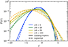Fig. 1 The density PDF for three Mach numbers. Solid lines portray the Castaing-Hopkins distribution as stated by Eq. (36), and dashed lines correspond to the log-normal PDF as stated by Eq. (2).

3.2 Comparison to the log-normal PDF

Figure 1 compares the two density PDF formulations for various Mach numbers. To compute the Castaing-Hopkins PDF, we have used S_δ = ln (1 + b²ℳ²) and a value for T_CH as in Eq. (37). Generally speaking, the two PDF make similar predictions at low densities. However, the shape of the two PDFs is quite different at high densities and this is more pronounced at higher Mach numbers. Consequently, the log-normal tends to overpredict the amount of very dense gas compared to the Castaing-Hopkins PDF. This, in turn, can drastically affect the estimated SFR.

3.3 The existing SFR models with the updated PDF

One can ask themselves what the existing star formation theories predict when replacing the log-normal PDF by the Castaing-Hopkins PDF. The answer is: an SFR which is practically zero. The KM and PN theories make use of a Mach number dependent critical density above which the density PDF has to be integrated. In the case of the Castaing-Hopkins PDF, we find from Eq. (36) that if $$\ln \left(\rho /{\rho }_0\right)>S_{\delta }/\left(2T_{\text{CH}}\left(1+T_{\text{CH}}\right)\right),$$

then 𝒫 = 0 and so is the SFR. We can rewrite Eq. (16) as ρ_crit/ρ₀ = K_critα_virℳ², where α_vir is the virial parameter and K_crit is a dimensionless factor on the order of unity. Combining the two expressions and using S_δ = ln(1 + b²ℳ²), we find that the SFR is zero when $$2T_{\text{CH}}\left(1+T_{\text{CH}}\right)\ln \left(K_{\text{crit\hspace{0.17em}}}{\alpha }_{\text{vir\hspace{0.17em}}}{ℳ}^2\right)>\ln \left(1+b^2{ℳ}^2\right)).$$

Typical values are K_critα_vir ≃ 1, b ≃ 0.5 whereas T_CH varies with the Mach number (see Fig. 3 of Hopkins 2013, Fig. 6 of Paper II and Eq. (37)). For Mach number around 20, T_CH will be close to 0.4. These numbers leads to the approximate condition $$\ln \left({ℳ}^2\right)>\ln \left(1+\frac{{ℳ}^2}{4}\right)\Rightarrow \frac{3}{4}{ℳ}^2>1,$$

which is easily satisfied. This implies that when applying the Castaing-Hopkins PDF, which is much more accurate than the usually employed PDF, the classical theories of the SFR lead to SFR = 0. Whereas this conclusion is exacerbated by the mathematical limit reached when u < 0, this nevertheless shows that the KM and PN density criteria must be revised and further stresses that simply taking a density threshold is not sufficient to build a consistent star formation theory. The comparison between models and the influence of the density PDF is further explored and discussed in Section 6.2.

4 A new estimate for the replenishment time

We now discuss the time that should be used to estimate the SFR in Eq. (23). In most theories, a freefall time estimated at some density is used. However, when a turbulent density PDF is used, the picture is not consistent. Since turbulence is responsible of setting the PDF, the time necessary to rejuvenate the dense gas should also be controlled by turbulence. In particular, since the dense gas is obtained by contraction of a large volume of diffuse gas, replacing the dense gas likely requires a large amount of time. The question that needs to be addressed is how much time does it take for a new piece of gas with the same density to be created by turbulent-induced contraction when a piece of fluid with a given density gravitationally collapses.

4.1 Analytical expression

We consider a clump of size R and density ρ. This clump was formed by the contraction of a larger clump of size R′ > R and density ρ′ < ρ. We assume turbulence is the main process that transforms a regular piece of gas into a collapsing piece of gas. Assuming that turbulence mainly induces one-dimensional contraction, we have R′/R = ρ/ρ′. The typical time to generate the clump at scale R from the clump at scale R′ is linked to the crossing time at scale R′: $${\tau }_{\text{cross\hspace{0.17em}}}\left(R^{\prime }\right)=\frac{R^{\prime }}{\sigma \left(R^{\prime }\right)}.$$(39)

With Eq. (4) and with R₀ = L_i, where L_i is the turbulence injection length assumed to be half the size of the system, we obtain $$\sigma \left(R^{\prime }\right)={\sigma }_0{\left(\frac{R^{\prime }}{L_i}\right)}^{{\eta }_v},$$(40)

where σ₀ is the average velocity dispersion of the entire cloud. This leads to the crossing time $${\tau }_{\text{cross\hspace{0.17em}}}\left(R^{\prime }\right)=\frac{L_i^{{\eta }_v}}{{\sigma }_0}{\left(R^{\prime }\right)}^{1-{\eta }_v}=\frac{L_i^{{\eta }_v}}{{\sigma }_0}{R}^{1-{\eta }_v}{\left(\frac{\rho }{{\rho }^{\prime }}\right)}^{1-{\eta }_v}.$$(41)

The gas of density ρ′ at scale R′ is transformed into gas of density ρ at scale R on a time τ_R′ with an efficiency ϵ(R, R′). Combining all this, we obtain the time estimate $${\tau }_{R,R^{\prime }}=\frac{{\tau }_{\text{cross}}\left(R^{\prime }\right)}{ϵ\left(R,R^{\prime }\right)}=\frac{L_i^{{\eta }_v}}{ϵ\left(R,R^{\prime }\right){\sigma }_0}{R}^{1-{\eta }_v}{\left(\frac{\rho }{{\rho }^{\prime }}\right)}^{1-{\eta }_v}.$$(42)

Now we must sum over all possible scales R′ or densities ρ′ from which the clump of size R with density could have formed, to get the mean τ. In this summation, it is necessary to weight the time τ_R,R′ by the gas mass of density ρ′ that exists at scale R′. This number is proportional to the mass-weighted density PDF ρ′𝒫(ρ′). This leads to $${\tau }_{\text{rep\hspace{0.17em}}}(R)=\frac{{{\displaystyle \int }}_{-\infty }^{\ln (\rho )}{\tau }_{R,R^{\prime }}{\rho }^{\prime }\mathcal{P}\left({\rho }^{\prime }\right)\text{d\hspace{0.17em}}\ln \left({\rho }^{\prime }\right)}{{{\displaystyle \int }}_{-\infty }^{\ln (\rho )}{\rho }^{\prime }\mathcal{P}\left({\rho }^{\prime }\right)\text{d\hspace{0.17em}}\ln \left({\rho }^{\prime }\right)},$$(43) $$=\frac{L_i^{{\eta }_v}}{{\sigma }_0}{R}^{1-{\eta }_v}{\rho }^{1-{\eta }_v}\frac{{\displaystyle {\int }_{-\infty }^{\ln (\rho )}ϵ}{\left(R,R^{\prime }\right)}^{-1}{\left({\rho }^{\prime }\right)}^{{\eta }_v}\mathcal{P}\left({\rho }^{\prime }\right)\text{d\hspace{0.17em}}\ln \left({\rho }^{\prime }\right)}{{\displaystyle {\int }_{-\infty }^{\ln (\rho )}{\rho }^{\prime }}\mathcal{P}\left({\rho }^{\prime }\right)\text{d\hspace{0.17em}}\ln \left({\rho }^{\prime }\right)},$$(44)

which is the mass-weighted time. The denominator ensures that the weight is normalized to 1.

Estimating the efficiency of the conversion of clumps, which at scale R′ have a density ρ′, into clumps which at scale R have a density ρ, is not an easy task, and we make several assumptions. First, we assume that it depends on the scale ratio ϵ(R, R′) = ϵ(R/R′). Second, we must have ϵ(x₁ x₂) = ϵ(x₁)ϵ(x₂), that is to say the efficiency between scale R₁ to R₃ is the product of the efficiencies between scales R₁ to R₂ and R₂ to R₃. Third, in the limit x → 1, we must have ϵ(x) → 1, whereas in the limit x → 0, ϵ(x) → 0. The solution to these constraints is e(x) = x^µ with µ > 0 which implies $$ϵ\left(R,R^{\prime }\right)={\left(\frac{R}{R^{\prime }}\right)}^{\mu }={\left(\frac{{\rho }^{\prime }}{\rho }\right)}^{\mu }.$$(45)

From numerical experiments, that is to say by confronting the analytical model with the simulation results, we found that µ is typically small and likely below 0.1. Therefore, in the following, for the sake of simplicity, we just assume µ = 0 and ϵ = 1. This expression leads to $${\tau }_{\text{rep\hspace{0.17em}}}(R)=\frac{L_i^{{\eta }_v}}{{\sigma }_0}{R}^{1-{\eta }_{\nu }}{\rho }^{1-{\eta }_{\nu }}\frac{{\displaystyle {\int }_{-\infty }^{\ln (\rho )}{\left({\rho }^{\prime }\right)}^{{\eta }_v}}\mathcal{P}\left({\rho }^{\prime }\right)\text{d\hspace{0.17em}}\ln \left({\rho }^{\prime }\right)}{{\displaystyle {\int }_{-\infty }^{\ln (\rho )}{\rho }^{\prime }}\mathcal{P}\left({\rho }^{\prime }\right)\text{d\hspace{0.17em}}\ln \left({\rho }^{\prime }\right)},$$(46)

which using Eq. (8) can be normalized as $${\tilde{\tau }}_{\text{rep}}(R)=\sqrt{\frac{32}{3\pi }}\frac{{\tilde{L}}_i^{{\eta }_v}}{ℳ}{\tilde{R}}^{1-{\eta }_v}{\tilde{\rho }}^{1-{\eta }_v}\frac{{{\displaystyle \int }}_{-\infty }^{\ln (\tilde{\rho })}{\left({\tilde{\rho }}^{\prime }\right)}^{{\eta }_v}\mathcal{P}\left({\tilde{\rho }}^{\prime }\right)\text{d\hspace{0.17em}}\ln \left({\tilde{\rho }}^{\prime }\right)}{{{\displaystyle \int }}_{-\infty }^{\ln (\tilde{\rho })}{\tilde{\rho }}^{\prime }\mathcal{P}\left({\tilde{\rho }}^{\prime }\right)\text{d\hspace{0.17em}}\ln \left({\tilde{\rho }}^{\prime }\right)}.$$(47)

Finally, as already explained, if the gravitational time is longer than the replenishment time, the SFR is controlled by the freefall time, and therefore the control time is given by τ_cont(R) = max(τ_rep(R), τ_ff (R)).

4.2 Comparison to the freefall time

To perform an estimate of the replenishment time, we use a turbulent driving length L_i equal to 200 pc, a number density of n₀ = 1.5 cm⁻³, four values of the Mach number and a compressibility described by the b parameter b = 0.67. We then use the mass-radius relation, Eq. (31). Figure 2 portrays the replenishment time, the freefall time and the control time as a function of the cloud mass. Except at relatively low Mach numbers and for massive clouds, the replenishment time is significantly longer than the freefall time. The reason is that as explained above, generating high density material is not a local process. It requires gathering the gas over large spatial scales. For high Mach number (ℳ > 20), the replenishment time is always the controlling time for star formation, and it only weakly depends on the structure’s mass.

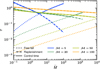Fig. 2 Replenishment time τrep (dashed line), freefall time τff (dotted lines) and control time τcont (solid lines) times for gravitationally unstable structures of mass M in a system with b = 0.67, Li = 200, n0 = 1.5 cm−3, and ηd = 0.5, using the Castaing-Hopkings PDF.

5 The mass spectrum of gravitationally unstable clumps

As discussed in Section 2, the HC SFR theory relies on the mass spectrum of collapsing clumps as expressed by the general Eq. (26). In their models, they assume a log-normal density PDF, however in Section 3 we saw how SFR models may change when using the Castaing-Hopkins PDF instead of the log-normal PDF. Therefore in this section we investigate how the mass spectrum changes when the Castaing-Hopkins PDF is utilized. Another important issue to which we pay attention as well, is the value of η_d and n_d = 3 + 2η_d, the exponent of the power-spectrum of ln ρ, which has usually been assumed to be identical to n_v the exponent of the power-spectrum of the velocity.

5.1 Calculating the mass spectrum

As discussed above, the mass spectrum, as stated by Eq. (26) presents two contributions. 𝒩₁ is proportional to the density PDF 𝒫 and can be easily computed once 𝒫 is known. To determine the term 𝒩₂, one first needs to calculate d𝒫_ℛ/dR and then perform an integration over densities. In some rare occasions, the second term could become negative, leading to some unphysi-cal features. In practice, when it is the case, we simply replace it by 0.

5.1.1 The mass spectrum for a log-normal PDF

Assuming a log-normal PDF and using Eqs. (26) and (27), the expression of the self-gravitating clump mass spectrum can be inferred. The integral in the term 𝒩₂ can be explicitly calculated (see Eqs. (13)–(15) of Hennebelle & Chabrier 2008). The expression of the corresponding mass spectrum is given in their appendix B and is equal to: $$\begin{array}{l}\tilde{\mathcal{N}}(\tilde{M})\simeq 2\frac{1}{{\tilde{R}}^3}\frac{1}{1+\left(2{\eta }_v+1\right){ℳ}_{\ast }^2{\tilde{R}}^{2{\eta }_v}}\\ \times \left(\frac{1+\left(1-{\eta }_v\right){ℳ}_{\ast }^2{\tilde{R}}^{2{\eta }_v}}{{\left(1+{ℳ}_{\ast }^2{\tilde{R}}^{2{\eta }_v}\right)}^{3/2}}-\frac{{\delta }_R^c+\frac{S_{\delta }{(R)}^2}{2}}{{\left(1+{ℳ}_{\ast }^2{\tilde{R}}^{2{\eta }_v}\right)}^{1/2}}\frac{n_d-3}{2}\frac{S_{\delta }\left(L_i\right)}{S_{\delta }(R)}{\left(\frac{\tilde{R}}{{\tilde{L}}_i}\right)}^{n_d-3}\right)\\ \exp \left(-\frac{{\left[\ln \left(\frac{\tilde{M}}{{\tilde{R}}^3}\right)\right]}^2}{S_{\delta }(R)}\right)\times \frac{\exp \left(-S_{\delta }(R)/8\right)}{\sqrt{2\pi S_{\delta }(R)}},\end{array}$$(48)

where $\mathcal{N}=\tilde{\mathcal{N}}/{\mathcal{N}}_0$, and ${\mathcal{N}}_0=\frac{{\rho }_0}{M_0^2},L_i=L_i/{\lambda }_{J,0}$, and, unlike Eq. (B1) of Hennebelle & Chabrier (2008), we have not assumed that n_v = n_d.

5.1.2 The mass spectrum for a Castaing-Hopkins PDF

The case of a Castaing-Hopkins PDF is somewhat cumbersome. Here we opt for a semi-numerical approach. The term 𝒩₁ in Eq. (26) is obtained through the Bessel function formulation stated by Eq. (38). The term 𝒩₂ entails $\frac{d{\mathcal{P}}_R}{dR}$. Using the Bessel function formulation from Eq. (38), we get $$\begin{array}{l}\frac{d{\mathcal{P}}_R}{dR}=\frac{\sqrt{\frac{\lambda }{u}}{e}^{-\lambda -u}}{T_{\text{CH}}}(\frac{I_0(2\sqrt{\lambda u})+I_2(2\sqrt{\lambda u})}{2}\hfill \\ +\left(-\frac{1}{T}\frac{d{T}_{\text{CH}}}{dR}+\left(\frac{1}{2\lambda }-1\right)\frac{d\lambda }{dR}-\left(\frac{1}{2u}+1\right)\frac{du}{dR}\right)I_1(2\sqrt{\lambda u})),\hfill \end{array}$$(49)

where we remind that $\lambda =S_{\delta }/\left(2T_{\text{CH}}^2\right)$ and where I₀, I₁ and I₂ are modified Bessel function of the first kind, which can be easily calculated using, for instance, the SCIPY python library. As can be noticed, one needs to know S_δ and T_CH as well as theirspatial derivative. We assume that T_CH varies with R the same way S_δ does (see Eq. (27)). The values S_δ(L_i) and T_CH(L_i) must also be specified and in this paper Eqs. (3) and (37) are employed. The final step to get N₂ requires an integration and this is done numerically using the quad function in the library SCIPY.

An alternative method to estimate 𝒩₂ is presented in Appendix A. It is based on the series formulation as stated by Eq. (36). It does not require further integral calculations but in practice computing the series appears to be time consuming.

5.2 Description and parameter dependence of the mass spectrum

5.2.1 Reference system

Here we study in detail a specific model which has L_i = 200 pc, n₀ = 1.5 cm⁻³ and a sound speed c_s = 0.3 km s⁻¹. These values roughly corresponds to the Milky Way which present a scale-height of about 100 pc, a mean density around 1 cm⁻³ and a temperature around 10 K for the cold and dense gas. We remind that what matters is ${\tilde{L}}_i=L_i/{\lambda }_{J,0}$ whose value in the present case is about 9. We assume that unstable structure can be found up to the injection scale L_i, or, in other words, y_cut = 1. We further assume a value of b = 0.5 which is expected for a mix of solenoidal and compressive modes. For η_v we take 0.4 which would lead to a velocity powerspectrum exponent of n_v = 3.8. For this set of parameters we explore a large range of Mach numbers going from ℳ = 5 to ℳ = 100.

Let us recall that the typical velocity dispersion in the Milky-Way is about 6–10 km s⁻¹ (Ferrière 2001) leading to Mach numbers, for the dense gas of about 20-30. We stress that in the ISM what is usually reported is either the Mach number at the scale of the disk scale height of the warm neutral medium or the Mach number at the scale of a cloud for the cold gas (e.g. Miville-Deschênes et al. 2017). In both cases, the inferred Mach numbers are smaller than 20 because in the first case the WNM has a sound speed of 8 km s⁻¹ , whereas in the second case, the cloud scale is smaller than the galactic scale height. The quoted Mach numbers of 20–30 are the ones that should be used to describe the motion of the cold gas at a scale comparable to the disk thickness. In high redshift galaxies, much larger velocity dispersion (e.g. Swinbank et al. 2012; Krumholz et al. 2018) have been reported leading to Mach numbers for the dense gas that can be up to 200.

In the top panel of Fig. 3, we show the resulting mass spectrum for this reference system when assuming either the log-normal PDF stated by Eq. (2) or the Castaing-Hopkins PDF stated by Eq. (36). We also explore two different ŋd values, 0.2 and 0.5. The choice of these values is motivated by the results from the simulations presented in Paper II.

5.2.2 Dependence on density PDF and Mach number

The results of the model which uses the Castaing-Hopkins PDF are quite different from what is predicted using the log-normal PDF, especially regarding the behaviour for increasing Mach number.

We see in Fig. 3 (top) that for ℳ = 5, both models predict similar mass spectra, since both PDFs are roughly equivalent at low Mach numbers. The mass spectrum presents a maximum around $\tilde{M}\simeq 1$ and sharply decreases for $\tilde{M}>1$. For ℳ = 20 and higher, the mass spectrum in the case of the log-normal PDF remains roughly unchanged for increasing M and follows a power law with an index of ≃ −1.5 until it steeply drops around $\tilde{M}\simeq {10}^3$.

However, when a Castaing-Hopkins PDF is employed, an additional cut-off at small masses emerges. This is directly attributable to the fact that the Castaing-Hopkins PDF contains less dense gas compared to the log-normal PDF. Indeed when the environment is very turbulent, the turbulent dispersion tends to stabilise clouds and fluctuations need to be denser to trigger gravitational collapse. The chance of finding such dense fluctuations is much lower for the Castaing-Hopkins PDF. The result is that only massive clouds are gravitationally unstable and the typical mass of a collapsing structure increases with ℳ.

5.2.3 Total amount of collapsing gas

In the bottom panels of Fig. 3, we show the cumulative distribution, weighted by the control time, which was discussed in Section 4. Note however that as seen in Figure 2 this time remains relatively constant for a large range of structure masses. These figures thus reflect the total mass of gravitationally unstable gas and give information about which structures contain the bulk of this collapsing material.

For low Mach numbers (5–20), the amount of self-gravitating gas is roughly independent of Mach number: the curves show a plateau at a normalised value of about 1, both for the log-normal and the Castaing-Hopkins PDF. For high Mach numbers on the other hand, there is less and less gravitationally unstable gas when the Mach number increases. The reduction is particularly dramatic when a Castaing-Hopkins PDF is employed as seen in the bottom right panel. This is a direct consequence of the fact that only massive clouds are gravitationally unstable in the case of the Castaing-Hopkins PDF. Such clouds are rare, in part due to the limited turbulence injection scale Li which is assumed to be roughly equal to the size of the astrophysical system. Turbulence cannot generate structures which are larger than the injection scale.

These observations already hint that there are two regimes for star formation depending on the Mach number. From low to intermediate values of ℳ the total mass of collapsing gas does not depend much on ℳ and thus the SFR should also not vary strongly with ℳ. At high Mach numbers however, the unstable structures have a size comparable to the size of the system (or say the turbulent driving scale) resulting in a low amount of collapsing gas and so we can expect the SFR to also drop sharply for increasing ℳ.

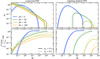Fig. 3 Mass spectra for various Mach numbers and PDF. Top: mass spectrum of self-gravitating structures. Bottom: time-weigthed cumulative mass spectrum of self-gravitating structures. Both quantities are plotted for a series of Mach numbers from ℳ = 5 (blue) to ℳ = 100 (orange), and for ηd = 0.2 (solid lines) and ηd = 0.5 (dotted lines). The models in the left column make use of the log-normal PDF while the ones in the right column use the Castaing-Hopkins PDF. For all curves, the compressibility parameter b is 0.67, the injection scale, Li, is assumed to be 200 pc and the mean density n0 is 1.5 cm−3.

5.2.4 Which clouds contribute to the SFR?

To understand which clouds contribute most to the reservoir of gravitationally unstable gas, and thus also the SFR, we look at the top and bottom panels together. On the one hand, we see that the cumulative distributions typically reach their plateau at masses that are somewhat below the extend of the high-mass tail of the mass spectrum. This means that the most massive clouds do not make a large contribution, mostly because such clouds are rare. We also observe that the contribution of low-mass clouds remains limited to 10% or less for a log-normal PDF, and is even lower in the case of the Castaing-Hopkins PDF. The dominant contribution thus comes from clouds of intermediate mass, relatively to the full range of the mass spectrum. The mass of the clouds that contribute the most thus increased with Mach number, especially for the Castaing-Hopkins PDF.

5.2.5 Dependence on the ln-density power-spectrum

In Fig. 3 we also compare the mass spectra obtained for η_d = 0.2 (solid lines) with those for η_d = 0.5 (dotted lines). We remind that η_d is linked to the exponent of the power-spectrum of ln ρ through Eq. (5). Thus the larger ηd, the more power there is on large scales implying that the density fluctuations tend to be bigger in size than for η_d = 0.2.

For low Mach numbers, the mass spectrum is almost identical for the two values of η_d. However for Mach number higher than 20, η_d has a significant effect on the shape, particularly at the high mass end. This leads to a strong influence on the total amount of self-gravitating gas, as can be seen in the cumulative distributions in the bottom panels of Fig. 3. For both PDF, there are more massive self-gravitating clouds with η_d = 0.5 than with η_d = 0.2, as we can expect from a steeper power spectrum. This is particularly important when a Castaing-Hopkins PDF is employed, since only large clouds are found to be gravitationally unstable. Having additional large scale structures dramatically increases the overall amount of collapsing gas.

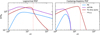Fig. 4 SFR as a function of Mach number. The left column is for log-normal PDF and the right column uses the Castaing-Hopkins PDF. TS stands for turbulent support (the present model), PN and mff PN models are discussed in Sect. 2.2. The employed value of b is 0.67, the value of ηd is 0.2, the injection scale Li, is assumed to be 200 pc and the mean density nc = 1.5 cm−3. The dotted line is the expected transition between the two regimes according to Eq. (55).

6 Resulting SFR model

In the previous sections, we have introduced the more accurate Castaing-Hopkins density PDF, an improved estimate for the replenishment time and have discussed the updated mass spectrum of gravitationally unstable structures. We now study the resulting SFR.

We remind that the SFR is estimated by Eq. (23), which sums the contributions of individual collapsing structures weighted by the appropriate characteristic time. The number of self-gravitating clumps, as generally given by Eq. (26), was calculated and discussed in Section 5, both in the case of a log-normal density PDF (Eq. (48)) and a Castaing-Hopkins PDF (calculated semi-analytically). The characteristic time, which as explained in Section 4, should not be simply the freefall time but rather the control time, τ_cont(R) = max(τ_rep, τ_ff) where τ_rep is the time needed to replace density fluctuations with a mass M_crit at scale R. The normalised SFR follows $$SF{R}_{\text{ff}}=SFR\frac{{\tau }_{\text{ff},0}}{{\rho }_0{L}_0^3}={{{\displaystyle \int }}^{\text{}}}_0^{{\tilde{M}}_{\text{sup\hspace{0.17em}}}}\frac{\tilde{\mathcal{N}}(\tilde{M})\tilde{M}}{{\tilde{\tau }}_{\text{cont\hspace{0.17em}}}(R)}\text{d}\tilde{M},$$(50)

where τ_ff,0 is the freefall time at the mean density ρ₀, whereas ${\rho }_0{L}_0^3$ is the total mass of the system. The bound of the integral, M_up, is obtained through the fact that R < R_cut = y_cutL_i together with Eq. (28), where y_cut is a dimensionless parameter that is typically below 1. The physical meaning of the y_cut parameter is that in a system in which the injection length of turbulence is L_i, it seems unlikely to have fluctuations of radius equal to L_i. The exact value of y_cut is however not known. When not specified we assume y_cut = 1 and we explore its influence in Section 7.3.

In this section, we investigate the SFR corresponding to the reference system defined in Section 5.2.1 with η_d = 0.5. In the first part, we demonstrate and discuss the emergence of two Mach number regimes. In the second part, we compare the results of our new model to the classical SFR models. In the next section, we explore the dependence on the system parameters.

6.1 The two regimes of the SFR

Figure 4 (red line) shows the resulting relation between the SFR and the Mach number for our newly introduced model, which results from Eqs. (26), (31) and (50). We name it the turbulent support (TS) model. As expected from the discussion of the cumulative mass spectrum in Section 5.2.3, we discover the existence of two regimes: for low Mach numbers the SFR is slightly increasing with ℳ, until a critical Mach number above which the SFR drops for increasing ℳ. The drop is particularly strong in the case of the Castaing-Hopkins PDF, which is due to the strong decrease in the total amount of collapsing gas as seen in the bottom panel of Figure 3.

While not the primary cause of the drop, the cut-off term 𝒩₂ for the mass spectrum does influence the severity of the SFR reduction at high Mach number. In Appendix B we show that without it, the SFR is a factor of about 3–4 larger in the high Mach regime.

The threshold Mach number which marks the separation between the two regimes is the same for both PDFs. To obtain a quantitative estimate for the transition Mach number, we can thus use the mathematical expressions for log-normal PDF, which are significantly simpler.

Mathematically, we see from Eq. (48) that the mass spectrum is composed of powerlaw terms and an exponential cut-off, which comes directly from the exponential in the log-normal PDF. An analogous cut-off manifests for the Castaing-Hopkins PDF. The powerlaw part of the mass spectrum corresponds to the density range around the peak of the log-normal PDF. Beyond that point, the number of structures drops steeply with increasing size as indeed seen as a high-mass cut-off in the top panel of Fig. 3.

To confirm that the high Mach number regime is indeed due to the steep decline of the density PDF at high density, we have computed the SFR using Eq. (48) for which the exponential term has been set to 1. In this case, it has been found that the SFR keeps increasing with the Mach number and that there is no steep decline contrary to what it is seen in Fig. 4. The exponential term responsible for cutting the cloud powerlaw distribution is $$E(\tilde{R})=\exp \left(-\frac{{\left(\ln \left(\tilde{M}/{\tilde{R}}^3\right)\right)}^2}{2S_{\delta }(\tilde{R})}\right)=\exp \left(-\frac{E_N(\tilde{R})}{2S_{\delta }(\tilde{R})}\right)$$(51)

where the scale-dependent variance $S_{\delta }(\tilde{R})$ is given by Eq. (27).

Using Eqs. (28), (33) and (4), the numerator $E_N(\tilde{R})$ becomes $$\begin{array}{l}{E}_N(\tilde{R})={\left(\ln \left(\tilde{M}/{\tilde{R}}^3\right)\right)}^2\\ \begin{array}{l}={\left[\ln \left({\tilde{R}}^{-2}\left(1+\frac{{ℳ}^2}{3}{\left(\frac{\tilde{R}}{{\tilde{L}}_i}\right)}^{2{\eta }_v}\right)\right)\right]}^2\hfill \\ \approx {\left[\ln \left(\frac{{ℳ}^2{\tilde{L}}_i^2}{3}{\left(\frac{\tilde{R}}{{\tilde{L}}_i}\right)}^{2\left({\eta }_v-1\right)}\right)\right]}^2\hfill \end{array}\end{array}$$(52)

when ℳ and $\tilde{R}$ are big enough. The exponential term $E(\tilde{R})$ will be very small unless $E_N(\tilde{R})\ll S_{\delta }(\tilde{R})$. The term $E_N(\tilde{R})$ is minimal when $\tilde{R}$ is close to ${\tilde{R}}_{\text{peak\hspace{0.17em}}}$² such that $${\tilde{R}}_{\text{peak\hspace{0.17em}}}={\left(\frac{ℳ{\tilde{L}}_i}{\sqrt{3}}\right)}^{1-{\eta }_v}{\tilde{L}}_i.$$(53)

From Eq. (27), we see that the variance $S\text{(}\tilde{R}\text{)}$ becomes zero in the limit $\tilde{R}\to {\tilde{L}}_i$. As a consequence, the mass spectrum is strongly reduced by the exponential term $E(\tilde{R})$ at all scales $\tilde{R}$ unless $${\tilde{R}}_{\text{peak\hspace{0.17em}}}<{\tilde{L}}_i.$$(54)

We note that if y_cut < 1, this condition becomes ${\tilde{R}}_{\text{peak\hspace{0.17em}}}<y_{\text{cut\hspace{0.17em}}}{\tilde{L}}_i$. Using Eq. (53) and assuming η_v < 1, we find that the condition (54) is equivalent to $$ℳ<{ℳ}_{\text{thres\hspace{0.17em}}}\text{\hspace{0.17em}where\hspace{0.17em}}{ℳ}_{\text{thres\hspace{0.17em}}}=\sqrt{3}{\tilde{L}}_i=\frac{L_i\sqrt{3G{\rho }_0}}{c_{\text{s}}}.$$(55)

When the Mach number is above ℳ_thres, the mass spectrum will be considerably attenuated by the term $E(\tilde{R})$: we enter the high-Mach regime, where star formation start to be inefficient. For our reference system with L_i = 200 pc the above-derived criterion results in ℳ_thresh ≈ 20, in excellent agreement with Fig. 4.

We can take a step back and look for a physical interpretation of our criterion. Rewriting Eq. (55), we see that star formation is efficient only if $$\frac{L_i}{{\lambda }_{J,0}}>\frac{ℳ}{\sqrt{3}},$$(56)

We note that in Eq. (56), the sound speed c_s appears both in λ_J,0 and in ℳ. By removing it on both sides, we can write that the transition between efficient and inefficient star formation occurs when the turbulent Jeans length is comparable to the injection length of turbulence: $$\frac{L_i}{{\lambda }_{\text{J},\text{\hspace{0.17em}turb\hspace{0.17em}}}}\simeq \frac{L_i}{\sigma /\sqrt{G{\rho }_0}}\simeq 1\text{,\hspace{0.17em}}$$(57)

where all numbers of order unity have been dropped.

This is very interesting because the turbulent Jeans length happens to be the scale where the turbulent velocity dispersion takes the role of the relevant speed to estimate the support against gravity.

Interestingly, the threshold Mach number depends only on the turbulence injection scale and the average density of the system. The details of the turbulence driving mechanism, that is the compressibility as well as the slope of the velocity or density power spectrum that is generated, play no role in setting the transition.

6.2 Comparison between models

Figure 4 also shows for comparison the PN and multi-freefall PN models (see Sects. 2.2 and 2.3 respectively) as a blue and purple curve. Clearly the behaviour of these two models is rather different compared to our new TS model (red line). At low ℳ, the mff PN and the TS model present comparable values, contrary to the PN model that typically produces lower values. When a log-normal PDF is employed (left panel) and for ℳ > 3–5, the SFR predicted by the models PN and multi-freefall PN monot-ically decrease with Mach number at a moderate rate, whereas the TS model starts to steeply drop.

As anticipated in Sect. 3.3, the difference is even far more dramatic when a Castaing-Hopkins PDF is employed as portrayed in the right panel. For ℳ > 6, due to small amount of dense gas predicted by this PDF, the PN and multi-freefall PN models lead to a vanishing SFR. Since the Castaing-Hopkins PDF has been found to be in much better agreement with simulation results than the log-normal, this constitutes a serious difficulty for this type of model that consists in estimating the SFR from the very dense gas.

The difference of behaviour between the three models is thus very significant. Let us remind that whereas the PN model consists essentially in estimating the very dense gas, gravitationally unstable at the thermal Jeans scale only, the TS model takes into account the gas unstable at all scales, in particular the gas supported by turbulence dispersion.

7 Influence of the model parameters on the SFR

In this section we examine how the various model parameters such as the power spectrum of the density field described by n_d or η_d, the maximum structure size described by y_cut, the turbulent forcing scale L_i and the mean density n₀, affect the relation between SFR and Mach numbers. Unless otherwise specified we use the parameters discussed in Sect. 5.2.

7.1 Dependence on the compressibility

Upper panel of Fig. 5 portrays the SFR as a function of Mach number for three values of the compressibility parameter b where S_δ = ln(1 + b²ℳ²). The values b = 0.33, 0.5 and 1 correspond to a purely solenoidal, mixed and purely compressive turbulence forcing (Federrath et al. 2008). The dot-dashed lines have been calculated using a log-normal PDF (Eq. (2)) and the solid lines used the Castaing-Hopkins PDF (Eq. (36)).

At low Mach number, the influence of b on the SFR remains limited. Only at high Mach number, that is for ℳ > 20 is there a significant difference. The steep dependence on Mach number in this regime originates from the stabilisation of massive clouds by turbulent support. This implies that denser perturbations must occur when the Mach number is larger. The probability of finding a denser fluctuation is higher when b is larger. For the same reason, there is a clear difference between the SFR calculated using the log-normal PDF and the Castaing-Hopkins PDF. While for low Mach numbers the Castaing-Hopkins PDF resembles a log-normal, for high Mach numbers the amount of dense gas is significantly reduced resulting in a lower SFR.

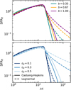Fig. 5 Predicted SFR for various parameters. Top: SFR for three values of b as a function of the Mach number (Li = 200, ηd = 0.2). Bottom: SFR for three values of ηd as a function of the Mach number (Li = 200, b = 0.67), where we remind that nd = 3 + 2ηd. Solid lines represent the model using the log-normal PDF and dot-dashed ones used the Castaing-Hopkins PDF.

7.2 Dependence on the logarithmic density powerspectrum

Lower panel of Fig. 5 displays the SFR as a function of Mach numbers for three values of η_d where we recall that n_d = 3 + 2η_d is the power-law exponent of the power-spectrum of In ρ. While there are almost no changes to the SFR when varying η_d in the low Mach regime, there is a very significant dependence for high Mach numbers. The reason is that larger η_d correspond to more numerous large scale density fluctuations which tend to be much more gravitationally unstable than smaller scale fluctuations. As discussed previously, the fluctuation distribution is really critical in the high Mach number regime.

This explains why the value of η_d has a strong impact.

In the high Mach regime and for the log-normal distribution, the SFR decreases significantly more steeply when η_d = 0.15 than for η_d = 0.3 or 0.5. This decrease is considerably steeper for the Castaing-Hopkins PDF and the dependence on η_d is less pronounced than for the log-normal PDF. Again this is a consequence of the high density part. The Castaing-Hopkins PDF presents less dense gas than the log-normal and therefore the amount of self-gravitating gas increases with η_d also less rapidly.

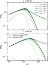Fig. 6 SFR for two values of Li, the injection length of turbulence, and four values of ycut, as a function of the Mach number. Solid lines represent the model using the Castaing-Hopkins PDF and dashed ones used the log-normal PDF. For all curves ηd = 0.5.

7.3 Dependence on the maximum structure size

Here we explore the influence of the y_cut parameter, which we remind defines the radius of the largest structures, R < y_cut L_i that are assumed to exist. In practice, the SFR defined by Eq. (50) is integrated up to M_sup, where M_sup is the mass associated to y_cut L_i through Eq. (28).

Figure 6 portrays the SFR as a function of Mach number for 4 values of y_cut. For y_cut > 0.5, the SFR does not depend strongly on it. The main effect of reducing y_cut is to smooth the transition between the low and high Mach regimes but otherwise the value of the SFR remains unchanged. This is however different for smaller values. For y_cut = 0.3, the SFR at large Mach is reduced whereas it remains unchanged at low Mach with respect to the case y_cut = 1. Finally, for y_cut = 0.1 and L_i = 200 pc, the SFR is lower at all Mach compared to the case y_cut = 1.

A priori, we do not know what the value of y_cut should be. We can imagine that the generation of the largest structures by turbulence is a stochastic process, meaning that some system may have a massive structures while other do not.

7.4 SFR as a function of mean density and turbulent driving scale

Here we explore further the dependence of the SFR on the density and driving scale with the goal of providing easy references to a large number of configurations. Figure 7 portrays the SFR as a function of Mach number for 3 values of L_i and several densities. We remind that the theory presented above depends on ${\tilde{L}}_i=L_i/{\lambda }_{J,0}$ and that the transition between the low and high Mach regimes broadly occurs when ${\tilde{L}}_i\simeq ℳ$.

The top panel displays the case L_i = 50 pc which broadly corresponds to the size of giant molecular clouds. We focus on three mean densities n₀ = 10, 30 and 100 cm⁻³, which are typical values for molecular clouds. As can be seen the behaviour of the SFR is similar to what has been previously inferred with a plateau at low to moderate Mach number followed by a steep drop at higher Mach numbers, which corresponds to a very inefficient star formation. We see that the Mach number at which the transition occurs is proportional to $n_0^{1/2}$ as expected from Eq. (55). Interestingly, rather low SFR values are obtained for values of ℳ ≃ 20 for n₀ = 10 cm⁻³ to ℳ ≃ 50 for n₀ = 100 cm⁻³. These values are typical of what is inferred for molecular clouds. For instance assuming that they follow Larson’s relations (Larson 1981; Hennebelle & Falgarone 2012), we expect a velocity dispersion on the order of 7 km s⁻¹ which given the assumed sound speed of 0.3 km s⁻¹ (relevant for the dense gas), leads to a Mach number of about 20, whereas the mean density at 50 pc is about 20 cm⁻³. Consequently, the present theory appears to be entirely compatible with the relatively low SFR inferred from observations (e.g. Lada et al. 2010).

The middle panel shows results for L_i = 200 pc, which again is comparable with (twice) the Galactic scale height. The densities that we considered are n₀ = 1, 3 and 10 cm⁻³ is typical to the density averaged at these scale in Milky-Way like galaxies.

Again the Mach numbers that corresponds to low SFR values are comparable to the ones observed in the Galaxy inside the solar circle (velocity dispersion of 10 km⁻¹ leading to ℳ ≃ 30).

The bottom panel portrays the SFR for L_i = 500 pc and densities equal to n₀ = 1,3 and 10 cm⁻³. As expected, the results are similar to the middle panel ones once the mach numbers are multiplied by a factor compatible with 500/200 = 2.5. The Mach number values are now quite high as getting a low SFR would require ℳ ≃ 100 or even larger depending of the density. Let us remind that very high velocity dispersions have been inferred in early type galaxies where velocity dispersions of up to 100 km s⁻¹ have been claimed (e.g. Swinbank et al. 2012; Krumholz et al. 2018).

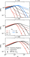Fig. 7 SFR for three values of Li, the injection length of turbulence, and several values of n0, the mean density, as a function of the Mach number. Solid lines represent the model using the Castaing-Hopkins PDF and dot-dashed ones used the log-normal PDF. For all curves ηd = 0.5. The star markers correspond to the Mach number which results from the mechanical equilibrium within a self-gravitating gas rich galactic disk as stated by Eq. (59).

8 Discussion

8.1 Criteria for inefficient star formation vs galactic vertical equilibrium

One of the main results of this paper is the existence of a high Mach regime which corresponds to a low SFR as explained in Section 6.1. In essence, if ${\tilde{L}}_i<ℳ/\sqrt{3}$, most of the density fluctuations are stabilised by the turbulent velocity dispersion. If galaxies are naturally in this high Mach number regime, it could explain their low observed SFRs.

The condition to be in the inefficient SFR regime presents strong similarities with the conditions for vertical equilibrium within a gas dominated galaxy. The gravitational potential, ϕ, is about ϕ ≃ 4πGρh², where h is the galaxy scale height. The mechanical equilibrium leads to $\varphi \simeq {\sigma }_{1D}^2$. Using the expression for the Jeans length, we get $${ℳ}_{\text{eq}}=\frac{\sqrt{3}\pi h}{{\lambda }_{J,0}}.$$(58)

Assuming that h ≃ L_i, that is to say the injection of turbulence is the smallest spatial scale of the system, we see that this leads to $${ℳ}_{\text{eq}}\simeq \sqrt{3}\pi {\tilde{L}}_i\simeq \pi {ℳ}_{\text{thres\hspace{0.17em}}},$$(59)

which therefore implies that ${\tilde{L}}_i<{ℳ}_{\text{eq}}/\sqrt{3}$ and thus that through vertical mechanical equilibrium, a galactic disk should naturally be in high Mach low SFR regime. The star markers in Fig. 7 display the equilibrium Mach number ℳ_eq corresponding to Eq. (59) and the expected SFR for a Castaing-Hopkins PDF. They show that a gas rich galactic disk is therefore expected to be in high Mach number regime meaning that an SFR_ff of about 0.3–0.4 could naturally result from the turbulent dispersion. Since in this regime the SFR sensitively depends on the Mach number, this estimate remains indicative. A detailed equilibrium and energy injection description is needed to infer more quantitative values. In particular, taking into account the stellar contribution for the gravitational potential, Eq. (59) would become $${ℳ}_{\text{eq}}\simeq \sqrt{3}\pi {\tilde{L}}_i\sqrt{1+\frac{{\rho }_{\ast }}{{\rho }_g}},$$(60)

where ρ_* is the mean stellar density, that is the mean density corresponding to the total stellar mass. This may indicate that the star markers in Fig. 7 have to be shifted to the right by a factor of about 3 resulting in even lower values of the SFR.

The conclusion that galactic disks in vertical turbulent equilibrium should naturally present a low star formation rate relies however on a strong assumption: that turbulent injection length is comparable to the disk thickness. Density fluctuations arising in the galactic disk plane could be significantly larger than the disk thickness, which would suggest that the relevant value of the turbulent injection scale L_i to consider is also larger than the disk thickness.

8.2 About considering powerlaw density PDF to calculate the SFR

It is now well established, both observationally (Kainulainen et al. 2009) and theoretically (Kritsuk et al. 2011; Lee & Hennebelle 2018) that in regions dominated by self-gravity, the density PDF develops a power-law tail as the result of gravita-tionnal collapse. Typically these power-laws have an exponent of about 3/2. This can be understood by the fact that a collapsing envelop tends to present a ρ ∝ r⁻² spatial profile. A uniform in-fall velocity combined with a density profile ∝ r⁻² leads to a constant accretion rate, which is probably why this type of solutions tend to appear (see for instance Larson 1969). Let us stress however that if ρ = Ar⁻², then energy conservation leads to $v_r=2\sqrt{2}\sqrt{\pi GA}$ and thus to an accretion rate Ṁ ∝ A^3/2. However, irrespective of the value of A, the density PDF is ∝ ρ^−3/2. This implies that the power-law tail of the PDF is highly degenerated regarding the SFR and may correspond to very different accretion rates. To illustrate this point further, we may for instance consider the self-similar isothermal collapse solutions (Larson 1969; Shu 1977). They all present densities, ρ ∝ r⁻², which in term of density PDF lead to a power-law tail ∝ ρ^−3/2 but their associated accretion rate may vary by orders of magnitude. This illustrates well that the power-law tail of the density PDF is a consequence of what is happening at larger scales. The larger scales are setting the SFR to which controls power-law tail. In principle, the latter should therefore be a prediction of the SFR theory.

Note however, that eventually the choice of considering a power-law tail to the PDF in order to estimate the SFR (Burkhart 2018) depends of the problem under investigation. For instance if ones wants to predict what the SFR within a molecular clouds for which such a power-law tail is observed, it could make perfect sense to include it because at the time of interest the star forming matter has already been assembled and the evolution time is not expected to be longer than a few cloud freefall times.

8.3 Possible further improvements

There are several possible lines of improvements that need to be explored in future studies. One of them is obviously taking into account the magnetic field which we have ignored here. It was considered in Hennebelle & Chabrier (2013) and could in principle be added easily. Its effect on the flow statistics (density PDF and power spectrum) should be studied as well (see Paper II). A recent study by Beattie et al. (2022) has revealed that there may be significant differences regarding the density PDF between hydrodynamics and MHD. This could also affect the value of ηd for instance.

Other important improvements would be accounting for stellar feedback, which has been found by many groups to significantly affect the SFR. This is true at the cloud scales (e.g. Wang et al. 2010; Nakamura & Li 2011; Federrath 2015; Verliat et al. 2022) in which case it is largely due to role of protostel-lar jets and at the galactic scales (e.g. Hopkins et al. 2011; Kim et al. 2013; Hennebelle & Iffrig 2014) where supernovae and HII regions are the dominant processes.

Similarly, it would be worth to account for temperature variations. This could possibly have a significant influence at low Mach numbers albeit the effect is probably limited in the high Mach regime identified in this paper.

Finally, we emphasize that it would be necessary to better understand and describe the transition from the low to the high Mach regimes. As discussed above this transition occurs when the size of the density fluctuations necessary to produce a self-gravitating clump is comparable to the size of the system which in turn is assumed to be the injection length of the turbulence. This is somehow accounted for by the density variance S_δ(R) which is presently described by Eq. (27). This however is most likely too simple to accurately described the distribution of spatial fluctuations comparable to the size of the system.

9 Conclusion

We have presented a new analytical model to predict the SFR in a turbulent environment. Contrary to previous propositions, our approach does not rely on a direct integration of the density PDF over a certain density threshold but rather on an estimate of the density fluctuations which at a given spatial scale are not supported against gravity either by thermal or turbulent support. We account for the density spatial distribution which is playing an important role regarding the value of the SFR because it affects the distribution of gravitationally unstable masses. We also revise the characteristic time that is relevant for the SFR arguing that this is not the freefall time but rather the time to replenish the amount of dense gas. Finally we also explore the influence of the density PDF proposed by Castaing (1996) and Hopkins (2013), which contains significantly less dense gas. We show that at high Mach number, it leads to substantial differences with the log-normal PDF.

We identify two different regimes of star formation that occur respectively at low and high Mach numbers. At low Mach numbers, our model predicts that the SFR is remarkably independent of ℳ. However, when the Mach number is higher than a threshold proportional to the injection length of the turbulence divided by the Jeans length, there is a steep decline of the SFR with ℳ. The reason is that because turbulent dispersion is accounted for in the model, the typical gravitationally unstable mass increases with ℳ. In the low Mach regime, increasing the Mach number will lead to the formation of larger and more massive unstable clouds without significantly changing the total unstable mass in the system. However, the maximal scale (and, consequently, the maximal mass) at which an unstable structure can be found is limited by the injection scale of the turbulence. When the Mach number is such that the turbulent Jeans length is larger than the turbulent injection length, only denser density fluctuations may possibly reach the mass needed for gravitational instability. Since according to the density PDF, the number of such fluctuations steeply falls, so does the SFR.

Data availability

The code to compute the TS model and to recreate the plots of this paper is available at https://gitlab.com/turbulent-support/ts_sfr_model.

Acknowledgements

This project was funded by the European Research Council under ERC Synergy Grant ECOGAL (grant 855130), led by Patrick Hennebelle, Ralf Klessen, Sergio Molinari and Leonardo Testi. The authors acknowledge Interstellar Institute’s program “II6” and the Paris-Saclay University’s Institut Pascal for hosting discussions that nourished the development of the ideas behind this work.

Appendix A SFR for the log-Poisson density PDF: The integral formulation

To obtain the SFR using the Castaing-Hopkins density PDF as stated by Eq. (36), it is necessary to calculate the term d𝒫_R/dR, which appears in Eq. (26).

Here we propose an integral formulation, in addition to the Bessel function formulation presented in Section 3, which can also be useful although the calculations are much longer than using Bessel functions available from mathematical packages. We have $$\begin{array}{l}\frac{d{\mathcal{P}}_R}{dR}(\delta )=\hfill \\ \frac{1}{T}{\displaystyle \underset{m=1}{{{{\displaystyle \sum }}^{\text{}}}^{\text{}}}}\left(mu-\lambda u+\frac{m-1}{1+T}\lambda -\frac{\lambda u}{1+T}\right)\frac{d\lambda }{dR}\frac{{\lambda }^{m-1}{e}^{-\lambda }}{m!}\frac{u^{m-2}{e}^{-u}}{(m-1)!}.\hfill \end{array}$$(A.1)

In Eq. (26), the quantity $${\displaystyle {\int }_{{\delta }_{\text{citit\hspace{0.17em}}}}^{\infty }d}\delta \exp (\delta )\frac{d{\mathcal{P}}_R}{dR}$$

appears and needs to be calculated. It itself requires to calculate the integral $$I_m={\displaystyle {\int }_{{\delta }_{\text{crit\hspace{0.17em}}}}^{{\delta }_{\max }}d}\delta \exp (\delta )u^m\exp (-u),$$(A.2)

where ${\delta }_{\max }=\frac{\lambda T}{1+T}$. Setting v = (1 + T)u, we obtain $$\begin{array}{l}{I}_m={{{\displaystyle \int }}^{\text{}}}_{{\delta }_{\text{citi\hspace{0.17em}}}}^{{\delta }_{\max }}d\delta \exp (\delta )u^m\exp (-u)\hfill \\ =\frac{T}{{(1+T)}^{m+1}}\exp \left({\delta }_{\max }\right){{{\displaystyle \int }}^{\text{}}}_0^{v_{\max }}{v}^m\exp (-v)dv,\hfill \end{array}$$(A.3)

where $v_{\max }=\lambda -\frac{T+1}{T}{\delta }_{\text{crit\hspace{0.17em}}}$. To calculate I_m we use $$\begin{array}{l}{J}_m={{{\displaystyle \int }}^{\text{}}}_0^a{v}^m\exp (-v)dv=m{J}_{m-1}-a^m\exp (-a),\hfill \\ J_0=1-\exp (-a).\hfill \end{array}$$(A.4)

This leads to $$\begin{array}{l}{{{\displaystyle \int }}^{\text{}}}_{{\delta }_{\text{citt\hspace{0.17em}}}}^{\infty }\exp (\delta )\frac{d{\mathcal{P}}_R}{dR}(\delta )d\delta ={{{\displaystyle \int }}^{\text{}}}_{{\delta }_{\text{crit\hspace{0.17em}}}}^{{\delta }_{\max }}\exp (\delta )\frac{d{\mathcal{P}}_R}{dR}(\delta )d\delta =\\ \frac{e^{-\lambda }}{T}\frac{d\lambda }{dR}{\displaystyle \underset{m=1}{{{\displaystyle \sum }}^{\text{}}}}\left(\left(m-\frac{\lambda (2+T)}{1+T}\right)I_{m-1}+\frac{\lambda (m-1)}{1+T}{I}_{m-2}\right)\frac{{\lambda }^{m-1}}{(m-1)!m!},\end{array}$$(A.5)

and $$\frac{d\lambda }{dR}=-\frac{{\sigma }_0^2}{2T^2}\left(n_d-3\right)\frac{R^{n_d-4}}{L_i^{n_d-3}}.$$(A.6)

Thus, with Eqs. (31,A.5), the mass spectrum is obtained from Eq. (26). To calculate Eq. (A.5), it is convenient to calculate $$\begin{array}{l}{K}_m=\frac{{\lambda }^m}{m!(m+1)!}{I}_m\hfill \\ =\frac{{\lambda }^m}{m!(m+1)!}{{{\displaystyle \int }}^{\text{}}}_{{\delta }_{\text{crit\hspace{0.17em}}}}^{{\delta }_{\max }}d\delta \exp (\delta )u^m\exp (-u)\hfill \\ =\frac{{\lambda }^m}{m!(m+1)!}\frac{T}{{(1+T)}^{m+1}}\exp \left({\delta }_{\max }\right){{{\displaystyle \int }}^{\text{}}}_0^{v_{\max }}{v}^m\exp (-v)dv\hfill \\ =\frac{{\lambda }^m}{m!(m+1)!}\frac{T}{{(1+T)}^{m+1}}\exp \left({\delta }_{\max }\right)\left(m{J}_{m-1}-a^m\exp (-a)\right)\hfill \\ =\frac{\lambda }{1+T}\frac{K_{m-1}}{m+1}-H_m,\hfill \end{array}$$(A.7)

and $$\begin{array}{l}{H}_m=\frac{a^m{\lambda }^m}{m!(m+1)!}\frac{T}{{(1+T)}^{m+1}}\exp \left(\frac{\lambda T}{1+T}-a\right)\hfill \\ =\frac{a\lambda }{m(m+1)(1+T)}{H}_{m-1}.\hfill \end{array}$$(A.8)

Thus we get $$\begin{array}{l}{{\displaystyle \int }}_{{\delta }_{\text{cit\hspace{0.17em}}}}^{\infty }\exp (\delta )\frac{d{\mathcal{P}}_R}{dR}(\delta )d\delta =\hfill \\ \frac{e^{-\lambda }}{T}\frac{d\lambda }{dR}{\displaystyle \underset{m=1}{{{{\displaystyle \sum }}^{\text{}}}^{\text{}}}}\left(\left(m-\frac{\lambda (2+T)}{1+T}\right)K_{m-1}+\frac{{\lambda }^2}{m(1+T)}{K}_{m-2}\right).\hfill \end{array}$$(A.9)

Appendix B The impact of the cut-off term on the SFR

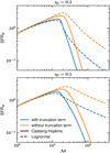Fig. B.1 Star formation rate as a function of Mach number. Dashed-lines correspond to the log-normal PDF and solid lines to the Castaing-Hopkins PDF. Blue lines stand for the complete expression of the SFR whereas orange lines represent the SFR obtained without the truncation term (see Eq. 26). The model parameters are L = 200 pc, b = 0.67, n0 = 1.5 cm−3 and ηd = 0.2 (top) or ηd = 0.5 (bottom).

As discussed in Sect. 3, the mass spectrum is composed of two terms. The second, which entails the derivative of the density PDF with respect to the spatial scale, is important only for spatial scales close to the injection length and it is playing a role in reducing the SFR. To explicitly study its influence, Fig. B.1 displays the SFR as a function of Mach number taking into account and excluding the cut-off term. Both the log-normal and the Castaing-Hopkins PDF are displayed. It appears that the cut-off term has a quantitative influence on the results but qualitatively the results are similar when it is accounted for and when it is not.

References

All Tables

All Figures

	Fig. 1 The density PDF for three Mach numbers. Solid lines portray the Castaing-Hopkins distribution as stated by Eq. (36), and dashed lines correspond to the log-normal PDF as stated by Eq. (2).
In the text

	Fig. 2 Replenishment time τrep (dashed line), freefall time τff (dotted lines) and control time τcont (solid lines) times for gravitationally unstable structures of mass M in a system with b = 0.67, Li = 200, n0 = 1.5 cm−3, and ηd = 0.5, using the Castaing-Hopkings PDF.
In the text

Fig. 3 Mass spectra for various Mach numbers and PDF. Top: mass spectrum of self-gravitating structures. Bottom: time-weigthed cumulative mass spectrum of self-gravitating structures. Both quantities are plotted for a series of Mach numbers from ℳ = 5 (blue) to ℳ = 100 (orange), and for ηd = 0.2 (solid lines) and ηd = 0.5 (dotted lines). The models in the left column make use of the log-normal PDF while the ones in the right column use the Castaing-Hopkins PDF. For all curves, the compressibility parameter b is 0.67, the injection scale, Li, is assumed to be 200 pc and the mean density n0 is 1.5 cm−3.

In the text

Fig. 4 SFR as a function of Mach number. The left column is for log-normal PDF and the right column uses the Castaing-Hopkins PDF. TS stands for turbulent support (the present model), PN and mff PN models are discussed in Sect. 2.2. The employed value of b is 0.67, the value of ηd is 0.2, the injection scale Li, is assumed to be 200 pc and the mean density nc = 1.5 cm−3. The dotted line is the expected transition between the two regimes according to Eq. (55).

In the text

	Fig. 5 Predicted SFR for various parameters. Top: SFR for three values of b as a function of the Mach number (Li = 200, ηd = 0.2). Bottom: SFR for three values of ηd as a function of the Mach number (Li = 200, b = 0.67), where we remind that nd = 3 + 2ηd. Solid lines represent the model using the log-normal PDF and dot-dashed ones used the Castaing-Hopkins PDF.
In the text

	Fig. 6 SFR for two values of Li, the injection length of turbulence, and four values of ycut, as a function of the Mach number. Solid lines represent the model using the Castaing-Hopkins PDF and dashed ones used the log-normal PDF. For all curves ηd = 0.5.
In the text

Fig. 7 SFR for three values of Li, the injection length of turbulence, and several values of n0, the mean density, as a function of the Mach number. Solid lines represent the model using the Castaing-Hopkins PDF and dot-dashed ones used the log-normal PDF. For all curves ηd = 0.5. The star markers correspond to the Mach number which results from the mechanical equilibrium within a self-gravitating gas rich galactic disk as stated by Eq. (59).

In the text

	Fig. B.1 Star formation rate as a function of Mach number. Dashed-lines correspond to the log-normal PDF and solid lines to the Castaing-Hopkins PDF. Blue lines stand for the complete expression of the SFR whereas orange lines represent the SFR obtained without the truncation term (see Eq. 26). The model parameters are L = 200 pc, b = 0.67, n0 = 1.5 cm−3 and ηd = 0.2 (top) or ηd = 0.5 (bottom).
In the text

References

- André, P., Men’shchikov, A., Bontemps, S., et al. 2010, A&A, 518, A102 [Google Scholar]
- Beattie, J. R., Mocz, P., Federrath, C., & Klessen, R. S. 2022, MNRAS, 517, 5003 [NASA ADS] [CrossRef] [Google Scholar]
- Braun, H., & Schmidt, W. 2015, MNRAS, 454, 1545 [NASA ADS] [CrossRef] [Google Scholar]
- Brucy, N., Hennebelle, P., Bournaud, F., & Colling, C. 2020, ApJ, 896, L34 [NASA ADS] [CrossRef] [Google Scholar]
- Brucy, N., Hennebelle, P., Colman, T., & Iteanu, S. 2023, A&A, 675, A144 [NASA ADS] [CrossRef] [EDP Sciences] [Google Scholar]
- Brucy, N., Hennebelle, P., Colman, T., Klessen, R. S., & Le Yhuelic, C. 2024, A&A, 690, A44 (Paper II) [NASA ADS] [CrossRef] [EDP Sciences] [Google Scholar]
- Burkhart, B. 2018, ApJ, 863, 118 [CrossRef] [Google Scholar]
- Castaing, B. 1996, J. Phys. II, 6, 105 [Google Scholar]
- Ciardi, A., & Hennebelle, P. 2010, MNRAS, 409, L39 [NASA ADS] [Google Scholar]
- Federrath, C. 2013, MNRAS, 436, 1245 [NASA ADS] [CrossRef] [Google Scholar]
- Federrath, C. 2015, MNRAS, 450, 4035 [Google Scholar]
- Federrath, C., & Klessen, R. S. 2012, ApJ, 761, 156 [Google Scholar]
- Federrath, C., & Banerjee, S. 2015, MNRAS, 448, 3297 [NASA ADS] [CrossRef] [Google Scholar]
- Federrath, C., Klessen, R. S., & Schmidt, W. 2008, ApJ, 688, L79 [NASA ADS] [CrossRef] [Google Scholar]
- Federrath, C., Roman-Duval, J., Klessen, R. S., Schmidt, W., & Mac Low, M. M. 2010, A&A, 512, A81 [NASA ADS] [CrossRef] [EDP Sciences] [Google Scholar]
- Ferrière, K. M. 2001, Rev. Mod. Phys., 73, 1031 [NASA ADS] [CrossRef] [Google Scholar]
- Hennebelle, P., & Chabrier, G. 2008, ApJ, 684, 395 [Google Scholar]
- Hennebelle, P., & Chabrier, G. 2011, ApJ, 743, L29 [Google Scholar]
- Hennebelle, P., & Chabrier, G. 2013, ApJ, 770, 150 [CrossRef] [Google Scholar]
- Hennebelle, P., & Falgarone, E. 2012, A&A Rev., 20, 55 [NASA ADS] [CrossRef] [Google Scholar]
- Hennebelle, P., & Iffrig, O. 2014, A&A, 570, A81 [NASA ADS] [CrossRef] [EDP Sciences] [Google Scholar]
- Hopkins, P. F. 2013, MNRAS, 430, 1880 [Google Scholar]
- Hopkins, P. F., Quataert, E., & Murray, N. 2011, MNRAS, 417, 950 [NASA ADS] [CrossRef] [Google Scholar]
- Iffrig, O., & Hennebelle, P. 2017, A&A, 604, A70 [NASA ADS] [CrossRef] [EDP Sciences] [Google Scholar]
- Kainulainen, J., Beuther, H., Henning, T., & Plume, R. 2009, A&A, 508, L35 [NASA ADS] [CrossRef] [EDP Sciences] [Google Scholar]
- Kennicutt, R. C., & Evans, N. J. 2012, ARA&A, 50, 531 [NASA ADS] [CrossRef] [Google Scholar]
- Kim, J., & Ryu, D. 2005, ApJ, 630, L45 [NASA ADS] [CrossRef] [Google Scholar]
- Kim, C.-G., Ostriker, E. C., & Kim, W.-T. 2013, ApJ, 776, 1 [NASA ADS] [CrossRef] [Google Scholar]
- Konstandin, L., Schmidt, W., Girichidis, P., et al. 2016, MNRAS, 460, 4483 [NASA ADS] [CrossRef] [Google Scholar]
- Kritsuk, A. G., Norman, M. L., Padoan, P., & Wagner, R. 2007, ApJ, 665, 416 [NASA ADS] [CrossRef] [Google Scholar]
- Kritsuk, A. G., Norman, M. L., & Wagner, R. 2011, ApJ, 727, L20 [NASA ADS] [CrossRef] [Google Scholar]
- Krumholz, M. R., & McKee, C. F. 2005, ApJ, 630, 250 [Google Scholar]
- Krumholz, M. R., Burkhart, B., Forbes, J. C., & Crocker, R. M. 2018, MNRAS, 477, 2716 [CrossRef] [Google Scholar]
- Lada, C. J., Lombardi, M., & Alves, J. F. 2010, ApJ, 724, 687 [Google Scholar]
- Larson, R. B. 1969, MNRAS, 145, 271 [Google Scholar]
- Larson, R. B. 1981, MNRAS, 194, 809 [Google Scholar]
- Lee, Y.-N., & Hennebelle, P. 2018, A&A, 611, A88 [NASA ADS] [CrossRef] [EDP Sciences] [Google Scholar]
- Mac Low, M.-M., & Klessen, R. S. 2004, Rev. Mod. Phys., 76, 125 [Google Scholar]
- Matzner, C. D., & McKee, C. F. 2000, ApJ, 545, 364 [NASA ADS] [CrossRef] [Google Scholar]
- Miville-Deschênes, M.-A., Murray, N., & Lee, E. J. 2017, ApJ, 834, 57 [Google Scholar]
- Mocz, P., & Burkhart, B. 2019, ApJ, 884, L35 [NASA ADS] [CrossRef] [Google Scholar]
- Nakamura, F., & Li, Z.-Y. 2011, ApJ, 740, 36 [NASA ADS] [CrossRef] [Google Scholar]
- Nordlund, Å. K., & Padoan, P. 1999, in Interstellar Turbulence, eds. J. Franco, & A. Carraminana, 218 [CrossRef] [Google Scholar]
- Nuñez-Castiñeyra, A., Nezri, E., Devriendt, J., & Teyssier, R. 2021, MNRAS, 501, 62 [Google Scholar]
- Padoan, P., & Nordlund, Å. 2011, ApJ, 730, 40 [Google Scholar]
- Press, W. H., & Schechter, P. 1974, ApJ, 187, 425 [Google Scholar]
- Renaud, F., Kraljic, K., & Bournaud, F. 2012, ApJ, 760, L16 [NASA ADS] [CrossRef] [Google Scholar]
- Schmidt, M. 1959, ApJ, 129, 243 [NASA ADS] [CrossRef] [Google Scholar]
- Schruba, A., Kruijssen, J. M. D., & Leroy, A. K. 2019, ApJ, 883, 2 [NASA ADS] [CrossRef] [Google Scholar]
- Shu, F. H. 1977, ApJ, 214, 488 [Google Scholar]
- Shu, F. H., Adams, F. C., & Lizano, S. 1987, ARA&A, 25, 23 [Google Scholar]
- Squire, J., & Hopkins, P. F. 2017, MNRAS, 471, 3753 [NASA ADS] [CrossRef] [Google Scholar]
- Sun, J., Leroy, A. K., Ostriker, E. C., et al. 2023, ApJ, 945, L19 [NASA ADS] [CrossRef] [Google Scholar]
- Swinbank, A. M., Sobral, D., Smail, I., et al. 2012, MNRAS, 426, 935 [NASA ADS] [CrossRef] [Google Scholar]
- Tatsumi, T., & Tokunaga, H. 1974, J. Fluid Mech., 65, 581 [NASA ADS] [CrossRef] [Google Scholar]
- Vazquez-Semadeni, E. 1994, ApJ, 423, 681 [Google Scholar]
- Verliat, A., Hennebelle, P., González, M., Lee, Y.-N., & Geen, S. 2022, A&A, 663, A6 [NASA ADS] [CrossRef] [EDP Sciences] [Google Scholar]
- Walch, S., & Naab, T. 2015, MNRAS, 451, 2757 [NASA ADS] [CrossRef] [Google Scholar]
- Wang, P., Li, Z.-Y., Abel, T., & Nakamura, F. 2010, ApJ, 709, 27 [NASA ADS] [CrossRef] [Google Scholar]
- Zuckerman, B., & Evans, II, N. J. 1974, ApJ, 192, L149 [NASA ADS] [CrossRef] [Google Scholar]
- Zuckerman, B., & Palmer, P. 1974, ARA&A, 12, 279 [NASA ADS] [CrossRef] [Google Scholar]
Besides, their fit was using values of ycut > 1 which does not make sense in the HC model framework.
would have been the maximum of
if
if  was a constant.