| Issue |
A&A
Volume 690, October 2024
|
|
|---|---|---|
| Article Number | A158 | |
| Number of page(s) | 26 | |
| Section | Galactic structure, stellar clusters and populations | |
| DOI | https://doi.org/10.1051/0004-6361/202450482 | |
| Published online | 04 October 2024 | |
Discrepancies between spectroscopy and HST photometry in tagging multiple stellar populations in 22 globular clusters
INAF-Osservatorio di Astrofisica e Scienza dello Spazio di Bologna, Via P. Gobetti 93/3, I-40129 Bologna, Italy
⋆ Corresponding author; This email address is being protected from spambots. You need JavaScript enabled to view it.
Received:
23
April
2024
Accepted:
3
June
2024
Abstract
Multiple populations (MPs) in globular clusters (GCs) are stars that are distinct for their abundances of light elements. The MPs can be directly separated by measuring abundances of C, N, O, Na, Al, and Mg with spectroscopy or indirectly from photometric sequences created by the impact of different chemistry on band passes of particular filters, such as the HST pseudo-colours in the ultraviolet. An attempt to link HST pseudo-colour maps (PCMs) and spectroscopy was made by Marino et al. (2019, MNRAS, 487, 3815), using abundances mostly from our FLAMES survey. However, we found that an incomplete census of stars in common was used in their population tagging. We corrected the situation by building our own PCMs and matching them with our abundances in 20 GCs, plus two GCs from other sources, doubling the sample with spectroscopic abundances available. We found that the pseudo-colour (magF275W − 2 × magF336W + magF438) does not have a monotonic trend with Na abundances, enhanced by proton-capture reactions in MPs. Moreover, on average about 16% of stars with spectroscopic Na abundances show a discrepant tagging of MPs with respect to the HST photometry. Stars with second generation (SG) chemistry are mistaken for first generation (FG) objects according to HST photometry and vice versa. In general, photometric indices tend to overestimate the fraction of FG stars, in particular in low mass GCs. We offer a simple explanation for these findings. Finally, we publish all our PCMs (with more than 31 800 stars in 22 GCs) with star ID and coordinates; this is done to ensure easy verification and reproduction, as should be the case in scientific papers.
Key words: stars: abundances / stars: atmospheres / stars: Population II / globular clusters: general
© The Authors 2024
 Open Access article, published by EDP Sciences, under the terms of the Creative Commons Attribution License (https://creativecommons.org/licenses/by/4.0), which permits unrestricted use, distribution, and reproduction in any medium, provided the original work is properly cited.
This article is published in open access under the Subscribe to Open model. This email address is being protected from spambots. You need JavaScript enabled to view it. to support open access publication.
1. Introduction
Multiple stellar populations (MPs) in Galactic globular clusters (GCs) are commonly defined as ensembles of cluster stars that are distinct for their light-element content. Striking differences in C and N content and Na and O content among GC stars have been known and studied since the 1980s (see Smith 1987; Kraft 1994 for reviews on those studies). Since the seminal paper by Gratton et al. (2001) on the abundances of unevolved stars in two clusters, it is crystal clear that presently evolving low-mass stars cannot be the origin of the observed chemical pattern. For the production of species such as N, Na, Al (and sometimes Si, Ca, Sc, K) combined with the simultaneous depletion of C, O, and Mg, Gratton et al. indicated that the most massive stars (now extinct) of a stellar population that preceded the one presently observed in GCs were responsible. The polluters among first-generation (FG) stars contributed matter nuclearly processed by proton-capture reactions in H-burning at high temperatures. Different cycles are involved, depending on the temperature thresholds achievable according to the polluter mass. The processed matter, coupled with diluting pristine gas, constitutes the necessary mass budget required to generate the subsequent second generation(s) (SG) with the observed chemical pattern (see e.g. the extensive reviews by Gratton et al. 2004, 2019, and references therein). In contrast to this widely accepted scenario, there is no consensus on a variety of issues regarding MPs; firstly, the nature of the polluters required to provide the raw material to be recycled into subsequent stellar generations or populations with modified composition. This mainly stems from the difficulties in matching (quantitatively, and sometimes qualitatively) theoretical models to the observed pattern of correlations and anti-correlations among light element abundances in GC stars (see e.g. Bastian & Lardo 2018). Thus, none of the many candidates proposed for FG polluters (e.g. intermediate-mass asymptotic giant branch, AGB, stars: Cottrell & Da Costa 1981; Ventura et al. 2001; massive, fast rotating stars: Decressin et al. 2007; massive binaries: de Mink et al. 2009; super-massive stars: Denissenkov & Hartwick 2014) seems to provide a fully satisfactory answer so far.
To gain more insight into MPs, it is useful to to study and compare the properties of distinct populations. The bedrock to this approach is identifying them with precision. In turn, the ratio of first-to-second generations is a key parameter to effectively constraining models to reconstruct the formation and early evolution of GCs. As an example, the extensive database of [O/Na] values spanned by different stellar populations in GCs allowed us to define the main property of MPs in GCs, that is that the relevance of the MP phenomenon is strictly correlated to the mass of the GC (Carretta 2006, Figures 12 and 13; Carretta et al. 2010a), a fact later confirmed by photometric means (e.g. Milone et al. 2017).
At the same time, the homogeneous tagging of stellar populations with primordial and altered chemical composition in a large set of GCs allowed us to draw attention to the so-called mass budget problem. Since the chemical composition of the polluted component must be inherited from only a part (the most massive) of an early stellar generation, the population ratio has a significant impact on every scenario devised to explain the formation of GCs, since it provides strong constraints on the initial GC mass. The proportion of FG and SG (about 30:70) stars derived from homogeneous spectroscopy and the Na−O anti-correlation implies that GCs could have initially been much more massive than today and that most of their FG low mass stars were lost at early times in the GC lifetime (e.g. Prantzos & Charbonnel 2006; Decressin et al. 2007; Carretta et al. 2010a; D’Ercole et al. 2010; Vesperini et al. 2010, 2013). It is thus of paramount relevance to correctly identify, among GC stars, those maintaining the original composition, which is identical to that of field stars of similar metallicity for all practical purposes, and those belonging to the next generation born in the cluster.
The main method used to tackle this issue is directly measuring the abundances of light elements with spectroscopy. Spectra, preferentially at high resolution for accurate abundances of atomic species, but even at low resolution for molecular features, allow us to directly separate stars with FG and SG chemical composition. Since different species are destroyed or produced at different temperatures, a complete survey of light element abundances is actually a tomography performed on the temperature distribution, and hence on the involved mass range, of the putative polluters.
Indirect measures are possible with photometry, exploiting filters with bandpasses that cover wavelength ranges affected by change in flux due to the effect of molecular bands, whose strength is modified by reactions enhancing N at the expense of depleting C and O. Hence, usually only UV and blue filters, encompassing the regions where OH, NH, and CN molecular features are located, are particularly efficient in this specific task. Several photometric systems have been used for this purpose (see e.g. Calamida et al. 2007; Sbordone et al. 2011; Carretta et al. 2011a; Lee et al. 2009; Massari et al. 2016 for ubvy Strömgren filters; Monelli et al. 2013 for the Johnson UBVI bands; Johnson et al. 2023 for the Sloan ugri system; and Piotto et al. 2015; Milone et al. 2017 for the combinations using ultraviolet HST filters).
Suitable combinations of magnitudes in these filters result in pseudo-colours able to separate photometric sequences mostly populated by stars of different compositions. The method uses appropriate normalisations suitable for clearly enhancing the separation of populations with different abundances of light elements, in particular C, N, and sometimes O.
Some photometric systems seem more suitable than others for providing accurate population tagging of stars in GCs (see e.g. Lee 2019, 2023), but recently the approach that uses UV, blue, and optical HST photometry has drawn much attention due to the large sample of GCs observed (57) and the exploitation of more absorbtion molecular bands in some suitable filters: OH in F275W, NH in F336W, CN and CH in F438W, and NH in F343W (the latter was employed by Larsen et al. 2014 to study GCs in the Fornax dwarf spheroidal galaxy).
The largest difference is obtained using a pseudo-colour derived by subtracting from the F275W magnitude (sensitive to the abundance of O, which is depleted in proton-capture reaction) two times the F336W magnitude (sensitive to N, which is enhanced) and finally adding the magnitude in F438W (whose bandpass includes a region of CH, another species that is depleted). Other, redder filters such as F814W are not particularly sensitive to the MP atmospheric composition, not including useful regions of molecular bands, but in combination with filters at much bluer wavelengths (e.g. F275W) are very sensitive to variations in the star’s effective temperature. In the assumption that the changes in light elements are accompanied by small differences in the He content, colours such as magF275W − magF814W, combining UV and optical bands, may provide some indications about He.
We now discuss notation. For clarity and conciseness, we adopt the simplifications illustrated in Table 1.
Notation adopted in the present paper.
The quantity col3 is called a pseudo-colour because it is actually the difference between two true colours. Formally, col is an actual colour, but similarly to the previous quantity it is used in a differential manner, as observed distances from a blue and a red ridge line in suitable colour-magnitude diagrams (CMDs); this is done for normalization purposes (see below, Section 2). The resulting combination is called a pseudo-colour map (PCM) in the following. On these maps, giant stars are generally located in two groups that are distinct along the ordinate by different values of Δcol3.
Simulations with synthetic spectra hint that this behaviour can mainly be attributed to variations in the N abundance (see e.g. Milone et al. 2017). Often, the two groups are rather well separated, but in some cases they seem to form almost a continuous sequence, with no clear evidence for separation. Interestingly, this does not seem clearly related to the cluster metallicity, which affects the detectability of bi-metal molecular features such as CN, as metal poor GCs may show a neat separation (such as, e.g. NGC 4833), while more metal-rich GCs (like NGC 6205) do not.
An attempt to link the photometric classification of MPs to the spectroscopic direct method was made by Marino et al. (2019), mostly using abundances from our extensive high-resolution FLAMES survey in GCs (Carretta et al. 2009a). However, we uncovered that a largely incomplete census of stars with abundances from spectroscopy was identified and used by Marino et al. (2019) to test the agreement of population tagging with the HST photometry.
We correct the situation in the present paper, using a full cross-matching of stars in common between the HST photometry and spectroscopy for 22 GCs among those used in Marino et al. (2019). For each analysed GC, Table 2 shows the number of stars with spectroscopic abundances individuated on the pseudo-colour maps of Marino et al. (2019) in the second column, and how many of them have [Fe/H] and [Na/Fe] ratios (third and fourth columns). In column 5, we report the number of stars we actually counted in the figures of the Na–Δcol3 relations shown by Marino et al. Columns 6–8 show how many stars with spectroscopic abundance we were able to match and use in the present work, while the references to the sources of abundance analysis are given in the last column. From this table, it is evident that Marino et al. (2019) neglected a large number of stars available in both the photometric and spectroscopic datasets.
Number of stars identified from spectroscopy in each GC.
In this work we focused on Na as a favoured indicator, as it is very well suited for tagging different stellar populations in GCs. Produced in the NeNa chain, it is tightly linked to the O depletion (providing the enhancement of N) in the Na−O anti-correlation, which is a feature found in almost every GC studied to date and such a key feature to be assumed as a true definition of genuine GCs (Carretta et al. 2010a). Sodium is not directly related to photometric sequences, but it is a good proxy for chemical alterations due to the MP phenomenon, maybe even better than O. Proton-capture reactions do enhance this species in SG stars with respect to the plateau imprinted by supernova nucleosynthesis, so the abundance of Na is easier to derive than that of other species depleted in the same nuclear processing, such as O. Furthermore, [Na/Fe] ratios can be reliably derived even in metal-poor GCs using the strong doublet at 5682−5688 Å, securing homogeneous abundances for the vast majority of GCs, down to the lowest metallicity objects.
Our analysis is organised in the paper as follows. In Section 2, we describe the data and the construction of the PCM. In Section 3, we show our first results on the comparison between the spectroscopic and photometric classification of MPs. These results are discussed in Section 4, where the population ratios obtained from different methods are tested against a sample of unpolluted, FG-like field stars. Our present work is summarised in Section 5.
2. The database of pseudo-colour maps (PCMs)
The only data published in Marino et al. (2019) are average abundances of elements from literature, largely from our FLAMES survey (Carretta 2006; Carretta et al. 2010a, and references therein). In particular, most Na abundances are from our analysis of GIRAFFE spectra in 15 GCs (Carretta et al. 2009a, see also Table 2). Unfortunately, no PCM has ever be made public by that collaboration, despite what was pledged in Piotto et al. (2015) and Marino et al. (2019). Although a PCM is sometimes used by other groups in the literature, the only public PCM we are aware of is the one of NGC 362 published by Vargas et al. (2022). We were then forced to construct our own PCM starting from scratch, exploiting the photometric catalogues of HST photometry in GCs by Nardiello et al. (2018) and following the procedure illustrated, for example, in Milone et al. (2017) and Dalessandro et al. (2019).
From the dataset of our FLAMES survey we selected 19 GCs with HST photometric catalogues in Nardiello et al. (2018) as target GCs. To this sample, we added two GCs with abundance analysis for a large number of stars from other sources (see Table 2) for consistency and safety verification. To this set, we added NGC 6388, whose large spectroscopic sample of 185 stars, studied in Carretta & Bragaglia (2023), was not available in 2019. For the 20 GCs in our survey, we used results from Carretta et al. (2009a), and other original papers of the series, adding data from Carretta et al. (2009b) for stars with only UVES spectra available. The photometric information (coordinates, magnitudes, and quality flags of stars) comes from the HUGS database; that is, the Large Legacy Treasury Program HST UV Globular Cluster Survey (Piotto et al. 2015; Nardiello et al. 2018).
2.1. Building a PCM
The procedure we followed is described here for one GC (NGC 104), and results for all clusters are presented in Appendix A. We downloaded the relevant files from the HST MAST archive1, choosing meth01, which is the most suitable for bright stars such as the RGB ones we dealt with. We selected stars in the RGB region using TOPCAT (Taylor 2005) and drew the blue and red fiducials for it. The lines were computed in magnitude bins (using magF814W) starting about 1.5 mag brighter than the main-sequence turn-off, taking the fourth and 96th percentiles in colour (col and col3; see Table 1 for the definition) of the stars in each bin. Some manual adjustments were made where too few stars were present; for instance, above the HB level in most clusters. We then used a polynomial interpolation to produce finer and smoother fiducial lines. An example of the procedure we followed is illustrated in Fig. 1, where we show these fiducials in the upper panels on the colour-magnitude diagrams (CMDs): col versus magF814W on the left and col3 versus magF814W on the right.
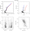 |
Fig. 1. Colour (and pseudo-colour) magnitude diagrams for NGC 104. The upper panels show the CMDs for NGC 104, col versus magF814W and col3 versus magF814W. The red and blue lines are the fiducials used. Lower left panels: rectified RGBs in the normalized col and col3. Lower right panel: resulting PCM, where FG stars are those located below approximately 0.1 in Δcol3 and SG stars above. |
No cut in photometric error was applied, as errors are tiny for bright stars (less or much less than 0.01 mag). Similar considerations are valid for other parameters such as sharpness or goodness of the PSF fits (quality; see Fig. 2). For each of the selected stars, we then computed the distance from the blue and red fiducials using Eqs. (1) and (2) in Milone et al. (2017; see also Table 1). To achieve the highest homogeneity possible, we adopted their widths of the RGB in col and in col3 (see Milone et al. 2017 for details and their Table 2 for the values).
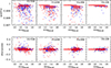 |
Fig. 2. Comparison of photometric parameters for the group of stars in all GCs with spectroscopy found in Marino et al. (2019; blue crosses) and those added only in the present work (red crosses), as a function of the magnitudes in F814W. The quality and sharpness parameters are from the catalogues of Nardiello et al. (2018) used to construct the PCMs. |
The corresponding Δcol and Δcol3 versus magF814W (i.e. the verticalised RGBs) are shown in the lower left panels of Fig. 1. Finally, the lower right panel of the figure shows the resulting PCM, where there is a separation of stars into two main groups, the one at lower Δcol3 values representing the FG stars and the one at higher Δcol3 values indicating the SG component (see Milone et al. 2017).
In Appendix A, we provide the same steps of the procedure for the remaining GCs. We will publish the whole set of PCMs for the entire sample of more than 31 800 giants in 22 GCs used in the present work at the CDS Strasbourg. This will be in the following format: Δcol, Δcol3, RA, Dec, ID, where ID is an eight-digit identifier from Nardiello et al. (2018), unique for each star in a given GC.
2.2. Cross-matching with the spectroscopic database
As the next step, we cross-matched the spectroscopic samples and the PCMs derived from HST photometry (see above) using TOPCAT (Taylor 2005) for each GC, retaining only stars in common (see Table 2 for the number of matches compared to the matches used in Marino et al. 2019). Beside simple matches of coordinates, we used the precaution of looking at the differences between the magF606W and the ground-based V magnitudes adopted in the individual papers. Large differences indicate a probable misidentification with a star within the separation range adopted for the match (1 arcsec), but this is usually much fainter than the spectroscopic target. In such cases, we inspected the possible different candidate matches, choosing the one possibly slightly more distant from the spectroscopic target, but within about 0.3−0.5 mag of its V magnitude, to allow for differences between the Johnson and the F606 HST filter.
No data or star identifications were published in Marino et al. (2019). However, from the figures shown in that paper, and knowing the Na, O abundances from the published papers, we were able to identify all stars used in Marino et al. in their comparison with spectroscopic results with confidence. A few problematic cases are reported and discussed in Appendix B.
In Table 3, we list the stars with both spectroscopy and HST photometry available in each of the 22 GCs of the present work. The star ID is from Nardiello et al. (2018), and it is unique within a given GC. Using this ID and the corresponding RA and Dec coordinates, it is easy to retrieve the stars from spectroscopic papers. The classification in MPs for each star (pop = 1 for FG and pop = 2 for SG stars) follows the spectroscopic criterion based on Na (see below). Flag = F indicate the stars found and used by Marino et al. (2019), identified through the position in their figures. The flag = M is used for additional stars in common between HST catalogues by Nardiello et al. (2018) and the papers of abundance analysis listed in Table 2, found by us and instead missing in Marino et al. Here, we show only the excerpt of Table 3 concerning NGC 104. The complete table is available at the CDS.
Stars with Na abundances retrieved in HST photometric catalogues (the complete table is available at the CDS).
As is clear from Table 2, there are many more stars with spectroscopic abundances than those used by Marino et al. (2019), even on the limited field of view sampled by HST observations. We were able to identify 298 stars used by Marino et al. among the 22 GCs of the present sample, all of them with a spectroscopic Na abundance2. To this set, we were able to add 291 stars (231 with Na), doubling the dataset of objects with both HST photometry and spectroscopy available. In the following, the stars used in the present work in addition to those adopted by Marino et al. are indicated in all the plots bordered in black.
It is not clear why Marino et al. (2019) neglected a large number of stars in each GC. To understand whether we selected stars differently from Marino et al. (2019), we checked the distribution of a few parameters on photometric quality and membership taken from the catalogues of Nardiello et al. (2018), used to construct the PCMs. In this exercise, we consider the stars with flag = F and those with flag = M as though they were different samples.
In Fig. 2, we compare the two photometric parameters sharpness and quality, as given by Nardiello et al. (2018), as a function of the magF814W. Blue crosses are for the limited sample of stars with spectroscopic abundances used in Marino et al. (2019). Red crosses indicate stars added in the present work. The two samples occupy essentially the same region.
The membership is compared in Fig. 3. The median value for the membership is the same for both groups, and a Kolmogorov-Smirnov test (bottom panel) returns a probability that does not allow us to reject the null hypothesis that the two samples are extracted from the same parent population. We further note that Marino et al. (2019) claimed that only stars that (according to their proper motion) are cluster members were included in their study. However, we uncovered that about 30 stars (∼11% of their adopted stars with spectroscopy) are listed in the catalogues by Nardiello et al. (2018) with mem = −1, meaning that the membership from proper motions is not available. A similar fraction (11%) is found among the stars added in the present work, increasing to about 13% when considering only stars with an Na abundance. Regardless of this, all stars with spectroscopy are cluster members according to their radial velocities and metallicities, which is probably a more robust criterion with respect to proper motions in particular within the crowded central regions of the GCs. Hence, we consider all the stars flagged either F or M as members, disregarding the statement by Marino et al. (2019).
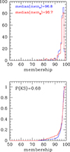 |
Fig. 3. Distribution of membership parameter from Nardiello et al. (2018) for stars only used by Marino et al. (2019: blue line) and only added in the present work (red line). Upper panel: Histogram of the membership parameters. Lower panel: Cumulative distribution. |
2.3. How to deal with very bright stars
A number of stars with spectroscopic abundances are flagged with ‘99’ in the catalogues by Nardiello et al. (2018), indicating that the stars in question are saturated in one or more frames. A posteriori, this is expected, since high signal to noise ratio (S/N) spectra are required to obtain accurate abundances at high resolution, and usually only the brightest stars are observed in GCs. Nevertheless, many of these bright stars were used by Marino et al. (2019), meaning that even these stars have a correspondence on their PCMs. Other bright stars were identified and added in the present paper.
Using the stars identified by Marino et al. (2019), we were able to place them on the PCM and in various diagrams, in particular the magF814W versus col3 diagram. The brightest stars follow a sharp turn to the left in the magF814W versus col3 diagram; so, conservatively we in primis truncated the RGB fiducial lines there when deriving the PCMs (see Fig. 1). However, when we counter-identified the stars observed spectroscopically, we saw that in half of the GCs many were close to this limit or exceeded it, even in the sample of stars used by Marino et al. (2019).
For those clusters (NGC 362, NGC 2808, NGC 4833, NGC 6093, NGC 6205, NGC 6388, NGC 6715, NGC 6809, NGC 6838, NGC 7078, and NGC 7099), we then extended the fiducial lines by eye to follow the RGB stars distribution. While not explicitly described in Milone et al. (2017) or Marino et al. (2019), this permitted us to place the stars in reasonable positions in the PCMs. An example of this is shown in Fig. 4 for NGC 2808, NGC 6205, and NGC 6715. Stars of the spectroscopic sample used in Marino et al. (2019) are over-plotted as larger filled symbols. Several stars in the saturated region are considered in the work of Marino et al., so they likely used the same procedure, extending the fiducial lines up to this region.
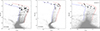 |
Fig. 4. Examples of saturation effect in col3, F814W plot for three GCs in our sample. Filled black circles are stars with spectroscopy available used by Marino et al. (2019). These stars also lie outside the vertical distribution of the RGB, so we extended the fiducial lines to bracket also these objects. |
2.4. A few words on the impact of reddening
As a general rule, we did not apply correction for reddening, since this would move all stars in the same way, while the essence of PCMs is working with differences with respect to fiducial sequences. However, we checked that disregarding the differential reddening present in a few GCs has no significant impact. We used NGC 3201, a cluster well known to be affected by differential reddening, and we applied a random variation of ±0.03 in the average E(B − V) for each star. This amount is compatible with the range of differential reddening recently found by Cadelano et al. (2024) over the limited HST field of view centred on this GC (about 0.06 mag peak-to-peak).
After this random addition, we repeated the complete procedure to build the new PCM of NGC 3201. The resulting PCM features resulted a little less compact, but perfectly able to separate FG from SG stars on this basis. This is enough for the goal of our paper, waiting for the publication of the precise, differential reddening-corrected PCMs by the Legacy Program group.
3. Spectroscopic and photometric classification of MPs
We now have at our disposal the newly derived PCMs, the stars with both photometry and spectroscopy available used by Marino et al., as well as the new additions (sometimes very numerous) presented in the present paper. This means that we have a large database of 22 GCs, whereby it is possible to compare the classification of MPs based on the HST photometry (indirect way) with that based on high-resolution spectroscopy (direct way). The comparison is shown in the next sections.
3.1. The Na–Δcol3 relations
As a first step to understanding the agreements or possible discrepancies in the classification of MPs with spectroscopy and photometry, we proceeded to scrutinise the Na–Δcol3 relations as a main diagnostic tool. In the pair of panels for each GC in Fig. 5, on the left we reproduce the relations exactly as given in Marino et al. (2019; their Figures 9 and 15). The first six GCs in our sample, NGC 104, NGC 288, NGC 362, NGC 1851, NGC 2808, and NGC 3201, are plotted in Fig. 5. In Figs. A.1 and A.2, we show the other GCs in our sample.
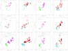 |
Fig. 5. Relations Δcol3–[Na/Fe] for NGC 104, NGC 288, NGC 362, NGC 1851, NGC 2808, and NGC 3201. For each GC, in the left panel the green and magenta symbols mark FG and SG stars, respectively, as classified from HST photometry (through the PCMs). The red triangles represent stars in the so-called red-RGB region. In the right panel, for each GC black circled symbols are stars in common between photometry and spectroscopy, yet they were neglected in Marino et al. Here, FG and SG stars (cyan and red, respectively) are separated according to the spectroscopic Na abundances (see text). |
The green and magenta colours are adopted for FG and SG stars, respectively, which have Na (and Fe) abundances from spectroscopy. Red triangles in NGC 362, NGC 1851, and NGC 6715 indicate stars located on the so-called red-RGB sequence, defined as an additional SG sequence above and to the red side of the main SG distribution by Milone et al. (2017).
In the left panels of each pair, the stars have both HST photometry and high-resolution spectroscopy, but the assignment to different populations was made in Marino et al. (2019) on a purely photometric basis; that is, stars belong to the FG or the SG group if they are located in the lower or upper ‘blob’ on the PCM, regardless of their actual chemical composition.
In order to also add stars missing from Marino et al., we had no choice but to use our own PCMs to associate a [Na/Fe] value with a given Δcol3 value. The resulting relations are plotted in the right panels of each pair of the above figures. We used the same scale as in the left panels. However, for NGC 2808 and NGC 6121 the scale of abscissa is different, to include all matches with our PCMs. Black bordered symbols indicate stars ignored by Marino et al. (2019) even if they have both photometric and spectroscopic data. The cyan and red colours mark FG and SG stars, respectively. However, now the populations are assigned based on a purely spectroscopic criterion.
According to the definition given in Carretta et al. (2009a), we selected stars in the FG (i.e. the primordial P component) with O, Na contents similar to field stars of the same metallicity. Stars are assigned to this component if their [Na/Fe] ratios lie in the range within [Na/Fe]min and [Na/Fe]min + 0.3 dex, where [Na/Fe]min is given by the lower envelope of the Na abundance observed in each GC. This criterion ensures that all the FG stars, with normal composition of halo stars, are included, since 0.3 dex is about 4σ([Na/Fe]), where σ([Na/Fe]) is the typical internal error on [Na/Fe] in our FLAMES survey. For consistency, we also applied the same criterion to the samples in NGC 6121 and NGC 6205, taken from other sources, but with similar internal errors on Na.
This selection offers a very homogeneous approach for all GCs in the sample, and it is based on Na abundances, that are well measurable even in the most metal-poor GCs, and are involved in the Na−O anti-correlation, a prominent feature of MPs in GCs. Its extension is found to be well correlated to the global GC mass (Carretta et al. 2010a, their Fig. 15), which is one of the main drivers of the MPs phenomenon, as inferred in a number of studies (Carretta 2006; Carretta et al. 2009a,b, 2010a; Pancino et al. 2017; Milone et al. 2017; Mészáros et al. 2020). Moreover, the choice of the minimum Na content in GCs of different metallicity allows us to follow the pattern of field halo stars derived from the plain Galactic chemical evolution. The soundness of the above criterion is proven by the good match between the FG fraction and the floor of unpolluted field stars over the whole metallicity range spanned by Galactic GCs (see Carretta 2016 and Section 4 in the present paper).
The relations shown by Marino et al. generally present a clean separation between FG and SG stars, with a sort of monotonic progression of Na abundances increasing as the Δcol3 values increase. Often there is a even a gap separating the two populations in this plane. This is simply a reflection of the adopted photometric criterion. On the PCM, the density thickening of stars corresponding to FG and SG stars shows only a slight superposition along the Δcol3 coordinate, and this explains the aspect of these relations. According to Figure 27 in Marino et al. (2019), the spread along the Δcol3 ordinate in the PCM is measuring essentially the variation in [N/Fe]. In proton-capture reactions in H-burning at high temperatures, both N and Na are enhanced (see e.g. Langer et al. 1993), in the ON cycle and NaNa chain, respectively, explaining the observed correlation.
Nonetheless, already at a glance the photometric classification of MPs shows several inconsistencies, which are visible in the Na–Δcol3 relations by Marino et al. (2019). Some FG stars (e.g. in NGC 6397, NGC 6752, and NGC 6838) have large Na abundances that are different from the low values typical of the primordial population. On the contrary, some SG stars show low Na abundances, consistent with the normal, unpolluted stellar population in GCs. A few objects are at the border between FG and SG stars, but in other cases (e.g. NGC 6093, NGC 6205, and NGC 6715) their Na abundance is clearly discrepant with respect to their photometric classification. Finally, we note that in some very metal-poor GCs (e.g. NGC 4590, NGC 7078), FG and SG stars are completely confused with each other, and both classes share the same range of Na abundances.
The monotonic progression in the Na–Δcol3 trend weakens when the tagging is done using the spectroscopic criterion, as in the right panels of each pair in Figures 5, A.1, and A.2. Despite a smooth increase of Na along the Na−O anti-correlation, often we do not observe a clean, almost one-to-one, correspondence. Instead, a large range of Na abundances corresponds to a given Δcol3 value, even reaching 0.7−1 dex in some cases.
Finally, in Fig. A.2 we show our result for NGC 6388. Marino et al. (2019) did not consider this GC, so there is no relation to Na–Δcol3 from their work. We exploited the large spectroscopic sample recently assembled in Carretta & Bragaglia (2023), and the relation is shown in the last panel of Fig. A.2 using the usual spectroscopic tagging, as in previous figures.
We conclude our analysis by noting that in NGC 2808 we see an FG star on the PCM of Marino et al. (2019), which then disappears in their Na–Δcol3 relation even if all the matches for NGC 2808 have an Na abundance. It was then impossible for us to identify this star. On the contrary, a few stars with spectroscopy used by Marino et al. (2019) in some GCs should not appear on the PCM, because they do not have all the required magnitudes in the catalogues by Nardiello et al. (2018). These and a few other peculiar stars are discussed in Appendix B.
3.2. Population classification on the PCMs
The enlarged sample of stars with spectroscopic abundances and our new PCMs available for the cross-identification of stars allow us to check, in detail, the agreement or differences arising from the classification of MPs using photometry or spectroscopy.
The comparison is shown for the first four GCs in Fig. 6. Figures A.3–A.7 are for the remainder of GCs. In the left panels, we reproduce the position on the PCMs of the stars with spectroscopic abundances used by Marino et al. (2019). Again, green and magenta colours are employed according to their photometric classification, disregarding direct measures of the chemical composition of stars. Adopting this classification, the FG stars generally have Δcol3 values lower than those of SG stars, likely due to lower N abundances in their chemical composition. However, this general rule has a few exceptions in about a third of the sample of GCs (e.g. NGC 2808, NGC 6093, NGC 6205, NGC 6254, NGC 6397, and NGC 7078). In these cases, FG and SG stars are found at the same level in Δcol3.
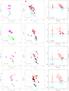 |
Fig. 6. Stars with spectroscopy on the PCMs of NGC 0104, NGC 288, NGC 362, and NGC 1851. In the left panels, the photometric classification of MPs is adopted; and in the middle panels, the population assignment is based on spectroscopy. Our PCMs are indicated with small grey dots. In the right panels, stars considered mismatches in classification are superimposed to the Na−O anti-correlation (as filled symbols). Solid lines in each GC indicate the limit [Na/Fe]min + 0.3 dex (with a range ±0.07 dex, dashed lines) used to separate FG and SG stars. The colour-coding is as in Fig. 5. |
In the central panels we plot the stars with spectroscopic abundances, superimposed on our PCMs (small grey dots). The colour-code for stars is the same as in Fig. 5 and follows the same assignment to MPs based on the [Na/Fe] abundance ratio as described in Section 3.1 and visualised in the panels on the right side for each GC. A solid line illustrates the criterion [Na/Fe]min + 0.3 dex used to separate FG stars (cyan open circles) from SG stars (red open circles). Dashed lines indicate the range ±0.07 dex around the separation, corresponding to the typical internal error on [Na/Fe] in abundance analyses from high-resolution spectra (e.g. Carretta et al. 2009a).
The spectroscopic classification of MPs is made ignoring, a priori, where the stars are located on the PCM, as this is based only on their Na content. This second approach immediately reveals a number of mismatches with respect to the population division of MPs based on photometry and, ultimately, on the effect of N abundances. Some stars belonging to the SG according to their enhanced Na are found on the PCM in the lower group, which should be populated by unpolluted stars with the normal composition of halo stars of similar metallicity. Vice versa, FG stars, which should display only the abundance pattern imprinted by supernovae nucleosynthesis, are found well inside the upper group on the PCMs; this is the one populated by giants with high or very high N abundances.
The observed mismatches in classification fall into two categories. We call those whose Na abundance is unambiguously distant from the dividing line of FG and SG stars (the separation of P and I components in the scheme defined in Carretta et al. 2009a) major mismatches. We define minor mismatches as those whose Na abundance lies within ±0.07 dex of the separation. In principle, this second class of misclassifications could be due to the star to star errors associated to the Na abundances. However, we note that the adopted criterion for the selection of FG stars ([Na/Fe]min + 0.3 dex) already includes a generous range of more than four times this internal error, so it is unlikely that some FG stars are missing. Moreover, the internal error in Na is by definition a random one, so we expect that FG stars near the separation are shifted upward or that SG stars are pushed downward simply from the associated error with the same probability; hence, statistically the neat effect is roughly unchanged.
On the other hand, a similar effect is present even in the photometric division of MPs, where a separation line between the two groups on the PCM is adopted with the same slope for all GCs, regardless of crowding, metallicity, or global GC mass, for example3. For the photometry of bright giants in GCs, the associated errors in magnitudes are usually minimal; however, the resulting observational error on Δcol3 (estimated from Fig. 2 of Milone et al. 2017 or Fig. 2 of Marino et al. 2019) amounts to about 0.05 mag on average. The meaning is that a similar drifting effect is also likely to impact the photometric fraction of MPs in GCs. Actually, in several GCs there are a few stars for which it is impossible to flag discrepancies or agreements between photometry and spectroscopy, simply because their belonging to either of the two groups in the PCM is unclear, as they fall equally far from both groups. To conclude, there could be a grey zone in both methods, where observational uncertainties may slightly blur the adopted criteria for population tagging. The majority of stars is nevertheless clearly distinct in both the photometric and spectroscopic approaches, allowing an useful comparison of their merits and drawbacks.
The mismatches in classification identified in the present sample of GCs are indicated on the Na−O anti-correlation (Fig. 6, and Figs. A.3–A.7) as filled symbols, coloured red or cyan according to their status as SG or FG stars following the Na criterion. In Table A.2, we list all stars whose classification differs between the HST photometry and the high-resolution spectroscopy. Using the information reported in this table, it is possible to situate each star on both our PCMs and on the Na−O anti-correlation. In Table A.2, we list the value of [Na/Fe]min + 0.3 dex and all the mismatches we found for each GC, with star ID, Δcol and Δcol3, the photometric classification based on PCMs, the [Na/Fe] and [O/Fe] ratios. Finally, a flag is used to label major mismatches with respect to the photometric population (labelled YES). The lowercase ‘yes’ warns us that the mismatch is a minor one.
Our enlarged sample in 22 GCs adds up to 529 stars with both an Na abundance and a pair of coordinates on the PCM. We found 75 mismatches in the population tagging on the whole; i.e. a fraction of 14 ± 2% (Poissonian error). Among these, 53 are major mismatches, and only 22 are minor mismatches, in the sense explained above. We are confident that even using the limit in Na as a strict condition is justified, and in the following we consider both categories together, except for noting if some results are affected by a particular prevalence by one of the types.
4. Discussion and conclusions
We quantify all the observed mismatches in the sample of GCs in Table 4, where we count both occurrences, i.e. SG stars from spectroscopy mimicking FG stars (according to HST photometry) and FG stars (according to their Na abundance) posing as SG stars on the PCMs. In Table 4, we report the fraction of these events in each GC in parentheses; this is computed over the total number of stars with the abundance of Na found in that GC. On average, over 20 GCs, the fraction of inconsistencies between the two methods of tagging is about 16%, ranging from a minimum of ∼4% (NGC 1851, NGC 2808, NGC 6121) to a rather impressive maximum of about 33% of stars in NGC 6809 and NGC 7078. The result does not depend much on the category of mismatch, with the average fraction being about 14.5% if we limit it to the major mismatches.
Number of mismatches between photometric and spectroscopic classification of MPs.
Despite the small numbers involved, the results summarized in Table 4 are informative. At first glance, it is possible to infer that the largest number of discrepancies between spectroscopy and HST photometry occurs among the most metal-poor GCs. This impression is visually confirmed in the left panel of Fig. 7, where the fraction of mismatches in the classification of MPs is plotted as a function of the metallicity of GCs. The [Fe/H] values are from our homogeneous metallicity scale based on high-resolution UVES spectra (Carretta et al. 2009c), with the exception of NGC 6205, which was taken from Johnson & Pilachowski (2012).
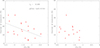 |
Fig. 7. Relation between fraction of mismatches in population tagging and the cluster metallicity. In the left panel, all the mismatches of Table 4 are counted, and the solid line is a linear fit to the data (Pearson correlation coefficient and the two-tail probability are labelled in the panel). In the left panel, fractions are computed using only major mismatches. |
There is a clear anti-correlation between the fraction of cases with a discrepant tagging of MPs and the cluster metallicity. Admittedly, the Poissonian errors associated with the fractions are rather large (about 8% on average), due to the limited number of cross-identifications between ground-based spectroscopy and the small field of view of HST observations, which are centred on the GC centres. However, the relation appears to be statistically significant. A linear regression returns a high value of the Pearson correlation coefficient with a significant two-tail probability that the relation is not due to a chance effect. Both values are indicated in Fig. 7, where the solid line indicates the regression. This figure shows that the fraction of stars misclassified on the PCMs, according to their Na abundance, is generally low in metal-rich or moderately metal-rich GCs, but it raises significantly among metal-poor GCs.
In the right panel of Fig. 7, the fraction is computed using only the major mismatches. We must duly note that the three most metal-rich GCs disappear, as does the statistical significance of the relation. Nevertheless, the trend still exists.
The increase in the number of discrepancies observed in more metal-poor GCs is compatible with the reduced response of RGB colours to the strength of the molecular bands, in particular the NH and CN features driving the behaviour of the Δcol3 coordinate on the PCM. The metallicity dependence of the band strength for bi-metal molecules varies quadratically with the metal abundance, so the tagging with the photometric classification is expected to be more fraught with uncertainties when the metallicity is decreasing (see e.g. the discussion in Lee 2023 about the increasing confusion in population tagging in some photometric systems for more metal-poor GCs).
In general, however, the relevant number of mismatches found between photometry and spectroscopy is somewhat surprising. The N abundance is the main source of the gross differences between FG and SG stars on the PCM, as this element directly affects the fluxes in the bands used to build the pseudo-colours and the resulting maps. The Na abundances do not directly affect the HST fluxes, but the correlation between this species and Δcol3 is a clear proxy of a correlation between Na and N.
A progressive enhancement of N along the RGB is expected in the normal evolution of low-mass stars, following the first dredge-up and another mixing episode after the luminosity bump level on the RGB (e.g. Charbonnel 1994; Gratton et al. 2000). However, the almost constant values of Δcol3 as a function of luminosity along the RGB (lower left panels in the figures of Appendix A) excludes that the observed pattern on the PCMs is related to any mixing episode. On the contrary, the variations in N must be intrinsic to the chemical composition of the whole star (Cohen et al. 2002) originated by the incomplete CN and ON burning at the same temperature at which the NeNa cycle is active.
As a consequence, the failure of PCMs to correctly locate stars according to their Na abundance in a non-negligible number of cases is at first glance a puzzle. The solution to this apparent riddle is uncovering the modern manifestation of the decoupling between N and heavier atomic species such as Na, which has been well known since the first studies on MPs (Smith et al. 2013; Smith 2015). Extensive works by Graeme Smith and collaborators unveiled that there is often a decoupling between the N abundances derived from molecular bands on one hand and the abundances of heavier elements such as O and Na on the other. This occurrence may be indicative of a complex enrichment by polluters with a range of masses and formation times within each GC.
The accurate comparison of C, N, and O, Na abundances in GC stars is neither easy nor immediate, since these elements are usually measured with different techniques, mostly low-resolution spectroscopy for the former pair and high-resolution spectroscopy for the second one. The comparison shown in Fig. 8 represents a typical case.
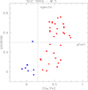 |
Fig. 8. Comparison of CN (Smith et al. 2013) and Na (Carretta et al. 2009a,b) indicators of MP tagging in NGC 5904 for stars in common between the two studies. The horizontal dashed line separates CN-strong (top) and CN-weak (bottom) stars, whereas blue and red filled circles represent FG and SG stars, respectively, as tagged by our spectroscopic criterion based on Na abundances (see Section 3.1). |
The CN index S(3839) for giants in NGC 5904 (Smith et al. 2013) measuring the λ3883 CN band strength is compared to Na abundances for RGB stars in common with Carretta et al. (2009a,b). To compensate at first order for the different effective temperature of RGB stars, the residuals with respect to the baseline defined by CN-weak stars as a function of magnitude, ΔS(3839), are used. The dashed horizontal line separates CN-weak and CN-strong stars, according to Smith et al. (2013). This level was labelled ‘phot’ because the criterion dividing FG, CN-weak stars from SG, CN-strong stars is basically the same, mainly tracing the N abundance derived by the incidence of molecular bands on photometric fluxes. The vertical line along the Na axis is labelled ‘spectr’ because the division is made using the criterion defined in Section 3.1 for the tagging of MPs based on Na abundances.
In Fig. 8, the same evidence given by the analysis of PCMs from HST photometry is reproduced. There is clearly a decoupling between the abundances of the lighter and the heavier proton-capture elements, superimposed on a global trend, with SG stars being more enhanced in CN and Na than FG, N-poor, Na-poor (and C-rich) stars. Even when N abundances are estimated from low-resolution spectroscopy, there are a few mismatches between the two classifications. A number of stars assigned to the FG according to their CN index have Na abundances as high as those classified as SG stars by both criteria. Conversely, in the pool of objects in common, one CN-strong star has [Na/Fe] compatible with the primordial level in NGC 5904. The effect is striking because 23Na is already produced through the destruction of 22Ne at 25 MK, whereas O achieves a depletion simultaneously. However, at the above temperatures the CN isotopes have already reached their equilibrium value (Prantzos et al. 2017).
In Fig. 9, the example of NGC 5904 is extended to four other GCs using a variety of different indicators for CN both from photometric systems or low-resolution spectroscopy in NGC 104, NGC 6205, NGC 6121, and NGC 6752. The separation between CN-strong and CN-weak stars are from the original papers. The first three GCs seem to show the same ‘pathology’ of NGC 5904, with a discrepant classification of FG and SG stars in a few cases. In all occurrences, CN-strong stars are found with low levels of Na.
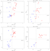 |
Fig. 9. Same as Fig. 8, but for four more GCs. Upper left panel: 47 Tuc, with CN index from Smith (2015) and O, Na from Cordero et al. (2014). Upper right panel: M 13, with CN index from Smith & Briley (2006) and O, Na from Johnson & Pilachowski (2012). Lower left panel: M 4, with CN index from Smith & Briley (2005) and O, Na from Marino et al. (2008). Lower right panel: NGC 6752, with CN index from Smith (2007) and O, Na from Carretta et al. (2007). |
Our definition of second generation(s) is based on the abundance variations of Na that distinguish stars with compositions altered by proton-capture reactions in GCs from their unpolluted counterparts, for example in the halo field. The comparison shown in Figs. 8 and 9 seems to point out that classification schemes based on CN indices, either photometric or spectroscopic, tend to overestimate the fraction of FG stars. This result is confirmed by the statistics concerning mismatches given in Table A.2. The vast majority of discrepancies (73 ± 10%) consist of stars erroneously classified as FG on the PCMs, whereas the contrary is only true for a minor fraction of the cases (27 ± 7%).
The impact of this unbalanced discrepancy on the population ratios of MPs in GCs is visualised in Fig. 10, where we plot the difference ΔFG in the unpolluted FG component as given by HST photometry (N1/Ntot, Milone et al. 2017) and as derived from the Na criterion (primordial P fraction; Carretta et al. 2010a and references in Table 2).
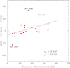 |
Fig. 10. Differences, ΔFG, in the fraction of FG stars from HST photometry through the PCMs and from the Na criterion as a function of the fraction of mismatches found in the present paper. A linear fit, with Pearson correlation coefficient and probability is also plotted. |
As the fraction of misclassification increases, the photometric method via PCMs increasingly overestimates the fraction of FG stars compared to the spectroscopic approach, and the trend is so regular that a simple linear regression turns out to be statistically significant (the Pearson correlation coefficient and the two-tail probability are reported in Fig. 10).
For the three major outliers in Fig. 10, NGC 288, NGC 2808, and NGC 6838, we compare the spectroscopic and photometric tagging of MPs in Fig. 11 using the sample of field stars assembled in Carretta (2013) for reference. This sample is homogenised to match the abundance analysis of GC stars as much as possible, so that the FG component in GCs individuated by Na only must be compatible with the floor of unpolluted field stars. In Fig. 11, red, blue, and green filled circles are used to represent the P, I, and E components defined in Carretta et al. (2009a). In particular, the primordial FG groups in each GC seem to be a fair match for the field counterpart (empty grey triangles). Filled black triangles indicate stars that seem to deviate from the bulk of distribution at a given metallicity. As discussed in Carretta (2013), they are composed by a sequence of stars whose origin is attributed to accretion. The horizontal red line in all the panels of Fig. 11 represents the level required by the estimates in Milone et al. (2017) to reproduce the fraction of FG stars derived from the PCMs in the spectroscopic sample.
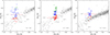 |
Fig. 11. Sodium distribution in the three GCs ouliers in Fig. 10 compared to the sample of field stars homogenized in Carretta (2013, triangles). Red, blue, and green filled circles are the P, I, and E components according to Carretta et al. (2009a). The red line reproduces the fraction of FG stars according to Milone et al. (2017) from PCMs (see text). From left to right, the panels are for NGC 288, NGC 2808, and NGC 6838. |
For the cases of NGC 288 (left panel) and NGC 6838 (right panel), the concept of primordial population according to the N-based selection from HST would include a consistent fraction of stars whose Na abundances clearly exceed the level imprinted in field stars by supernovae nucleosynthesis only. We remind the reader that several studies found that a mere 2 − 3% of halo stars show a chemical composition typical of SG stars in GCs (e.g. Carretta et al. 2010a; Martell et al. 2011; Koch et al. 2019). On the contrary, in NGC 2808 (middle panel of Fig. 11) the HST classification would leave out a significant number of FG stars with compositions identical to that of unpolluted field stars, in order to reproduce the low fraction (about 23%) quoted in Milone et al. (2017). We must note that the unusually low FG fraction for NGC 2808 appears to be at odds with most of the determinations from both spectroscopy and photometry (see Table 9 in Carretta 2015).
How much CN-based evaluations may overestimate the FG fraction with respect to the GC global characteristics can be evaluated from Fig. 12, where we show the difference ΔFG as a function of the total absolute magnitude for the 22 GCs in the present study. The total luminosity is a proxy of the present-day mass of GCs, but the trend exists, and it is equally statistically significant when using the initial masses of GCs as listed in the database by H. Baumgardt4. Our previous studies based on the Na−O anti-correlation detected a fraction of the primordial P component essentially constant in GCs (about 30% of stars); so, the trend observed above is hardly surprising given that Milone et al. (2017) found, from their PCM estimates, a trend where N1/Ntot increases in the lower mass GCs.
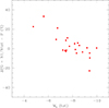 |
Fig. 12. Differences ΔFG as a function of the total absolute magnitude of the 22 GCs in this study. |
To conclude, the N-based methods of population tagging for MPs tend to overestimate the fraction of FG stars, and this tendency seems to be more frequent in more metal-poor and less massive GCs. As a consequence, the fraction of SG stars in these GCs is underestimated. For the high-mass GCs such as NGC 2808, this trend could even be reversed, although data are still too sparse for a firmer conclusion. The scenario is made more complex by the need to dilute the matter processed in proton-capture reactions (in polluters whose exact nature is still unknown) with pristine gas in GCs (whose abundance can be only guessed).
5. Summary
We addressed the issue of population tagging of MPs in GCs using different methods. For this purpose, we compared indicators based on HST photometry and direct probes of MPs such as the Na abundance from high-resolution spectroscopy.
Due to the lack of published data, we derived PCMs for 22 GCs with photometric catalogues from Nardiello et al. (2018). To check how photometric indicators perform in the population tagging, the photometry was then matched with stars having Na abundances mostly from our very homogeneous FLAMES survey. With respect to a similar attempt by Marino et al. (2019), we retrieved all the stars they used with both HST photometry and high-resolution spectroscopy available and added a new sample of matches, doubling the database of cross-identifications between photometry and spectroscopy. Our conclusions can be summarised as follows:
-
(1)
Our analysis shows that PCMs perform a coarsely correct ranking in populations for the bulk of stars in GCs, based essentially on the pseudo-colour col3 sensitive to N abundances through the effect of NH and CN molecular bands on fluxes in proper bandpasses.
-
(2)
When the classification from PCM is compared to the direct individuation of MPs from spectroscopic abundances, there are a number of mismatches or misclassifications, in particular when Na is used as privileged species to disentangle FG and SG stars. Stars populating the SG region are found with low Na abundances whereas stars belonging to the PCM region of FG stars have Na abundances at the level of stars with content of light elements clearly altered by proton-capture reactions responsible for the MPs phenomenon. The latter group constitutes the majority of the observed misclassifications.
-
(3)
On average, we found that about 16% of stars with spectroscopic abundances are erroneously classified in PCMs. The fraction of mismatches increases in metal-poor GCs, suggesting that the weakening of molecular features may play a role in the misclassification.
-
(4)
Hence, the estimates of the fraction of FG stars are different when using different indicators. Those based on NH or CN (hence the majority from UV or optical photometry) are usually higher than those from pure spectroscopic abundances from heavier elements. The comparison with the unpolluted floor as given by halo field stars shows that photometric tagging tends to overestimate the FG fraction.
-
(5)
The difference in estimates seems to vary from cluster to cluster, according to the cluster total mass. The overestimation of the FG fraction seems to be quantitatively more severe and pronounced in more metal-poor and less massive GCs.
To conclude, what we found in the present work is the modern form assumed by the well-known decoupling observed in abundances of N and Na among the MPs in GCs. We confirm the early extensive studies by Smith and collaborators: the phenomenon as seen by CN and O, Na is the same, namely with regard to the multiple stellar populations in GCs, but different aspects are likely sampled by the lighter and the heavier proton-capture elements.
The PCMs seem to follow only the outcome of the C−N cycle at moderate or low temperatures (T > 10 MK for C→N processing) rather well. When going to higher temperature regimes, where both the O−N cycle and the Ne−Na chain are at work (T > 40 MK), there are mistakes in the classification and usually stars with Na abundances high enough to be located in the SG region along the Na−O anti-correlation are mistaken for FG stars.
This finding represents a strong caveat for all the issues concerning the correct population ratios in MPs, such as the mass budget problem, since the FG fraction is the pool from which some massive polluters provide the nuclearly processed matter to be used, together with pristine gas, for the assembly of the stellar population with altered chemical composition. Despite some decades of observations from both photometry and spectroscopy gained for GC stars, the issue of MPs seems to be, even now, still far from being solved. Finally, we note that all the conclusions made in the present work have only been possible thanks to publicly available data.
Data availability
Full Tables 3 and A.1 are available at the CDS via anonymous ftp to cdsarc.cds.unistra.fr (130.79.128.5) or via https://cdsarc.cds.unistra.fr/viz-bin/cat/J/A+A/690/A158
This assumption clashes with the knowledge that the Na−O anti-correlation, albeit universal among GCs, is different in extent and shape from cluster to cluster.
Acknowledgments
This research has made large use of the SIMBAD database (in particular Vizier), operated at CDS, Strasbourg, France, of the NASA’s Astrophysical Data System, and TOPCAT.
References
- Bastian, N., & Lardo, C. 2018, ARA&A, 56, 83 [Google Scholar]
- Bragaglia, A., Carretta, E., D’Orazi, V., et al. 2017, A&A, 607, A44 [NASA ADS] [CrossRef] [EDP Sciences] [Google Scholar]
- Cadelano, M., Dalessandro, E., & Vesperini, E. 2024, A&A, 685, A158 [NASA ADS] [CrossRef] [EDP Sciences] [Google Scholar]
- Calamida, A., Bono, G., Stetson, P. B., et al. 2007, ApJ, 670, 400 [Google Scholar]
- Carretta, E. 2006, AJ, 131, 1766 [Google Scholar]
- Carretta, E. 2013, A&A, 557, A128 [NASA ADS] [CrossRef] [EDP Sciences] [Google Scholar]
- Carretta, E. 2015, ApJ, 810, 148 [Google Scholar]
- Carretta, E. 2016, IAU Symp., 317, 97 [Google Scholar]
- Carretta, E., & Bragaglia, A. 2023, A&A, 677, A73 [NASA ADS] [CrossRef] [EDP Sciences] [Google Scholar]
- Carretta, E., Bragaglia, A., Gratton, R. G., Lucatello, S., & Momany, Y. 2007, A&A, 464, 927 [NASA ADS] [CrossRef] [EDP Sciences] [Google Scholar]
- Carretta, E., Bragaglia, A., Gratton, R. G., et al. 2009a, A&A, 505, 117 [NASA ADS] [CrossRef] [EDP Sciences] [Google Scholar]
- Carretta, E., Bragaglia, A., Gratton, R. G., & Lucatello, S. 2009b, A&A, 505, 139 [NASA ADS] [CrossRef] [EDP Sciences] [Google Scholar]
- Carretta, E., Bragaglia, A., Gratton, R. G., D’Orazi, V., & Lucatello, S. 2009c, A&A, 508, 695 [NASA ADS] [CrossRef] [EDP Sciences] [Google Scholar]
- Carretta, E., Bragaglia, A., Gratton, R. G., et al. 2010a, A&A, 516, A55 [NASA ADS] [CrossRef] [EDP Sciences] [Google Scholar]
- Carretta, E., Bragaglia, A., Gratton, R. G., et al. 2010b, A&A, 520, A95 [NASA ADS] [CrossRef] [EDP Sciences] [Google Scholar]
- Carretta, E., Bragaglia, A., Gratton, R. G., D’Orazi, V., & Lucatello, S. 2011a, A&A, 535, A121 [NASA ADS] [CrossRef] [EDP Sciences] [Google Scholar]
- Carretta, E., Lucatello, S., Gratton, R. G., Bragaglia, A., & D’Orazi, V. 2011b, A&A, 533, A69 [NASA ADS] [CrossRef] [EDP Sciences] [Google Scholar]
- Carretta, E., Bragaglia, A., Gratton, R. G., et al. 2013, A&A, 557, A138 [NASA ADS] [CrossRef] [EDP Sciences] [Google Scholar]
- Carretta, E., Bragaglia, A., Gratton, R. G., et al. 2014, A&A, 564, A60 [NASA ADS] [CrossRef] [EDP Sciences] [Google Scholar]
- Carretta, E., Bragaglia, A., Gratton, R. G., et al. 2015, A&A, 578, A116 [CrossRef] [EDP Sciences] [Google Scholar]
- Charbonnel, C. 1994, A&A, 282, 811 [NASA ADS] [Google Scholar]
- Cohen, J. G., Briley, M. M., & Stetson, P. B. 2002, AJ, 123, 2525 [NASA ADS] [CrossRef] [Google Scholar]
- Cordero, M. J., Pilachowski, C. A., Johnson, C. I., et al. 2014, ApJ, 780, 94 [Google Scholar]
- Cottrell, P. L., & Da Costa, G. S. 1981, ApJ, 245, L79 [NASA ADS] [CrossRef] [Google Scholar]
- Dalessandro, E., Cadelano, M., Vesperini, E., et al. 2019, ApJ, 884, L24 [Google Scholar]
- Decressin, T., Meynet, G., Prantzos, Charbonnel C. N., & Ekstrom, S., 2007, A&A, 464, 1029 [NASA ADS] [CrossRef] [EDP Sciences] [Google Scholar]
- de Mink, S. E., Pols, O. R., Langer, N., & Izzard, R. G. 2009, A&A, 507, L1 [NASA ADS] [CrossRef] [EDP Sciences] [Google Scholar]
- Denissenkov, P. A., & Hartwick, F. D. A. 2014, MNRAS, 437, L21 [Google Scholar]
- D’Ercole, A., D’Antona, F., Ventura, P., Vesperini, E., & McMillan, S. L. W. 2010, MNRAS, 407, 854 [Google Scholar]
- Gratton, R. G., Sneden, C., Carretta, E., & Bragaglia, A. 2000, A&A, 354, 169 [NASA ADS] [Google Scholar]
- Gratton, R. G., Bonifacio, P., Bragaglia, A., et al. 2001, A&A, 369, 87 [NASA ADS] [CrossRef] [EDP Sciences] [Google Scholar]
- Gratton, R. G., Sneden, C., & Carretta, E. 2004, ARA&A, 42, 385 [Google Scholar]
- Gratton, R. G., Bragaglia, A., Carretta, E., et al. 2019, A&ARv, 27, 8 [Google Scholar]
- Johnson, C. I., & Pilachowski, C. A. 2012, ApJ, 754, L38 [NASA ADS] [CrossRef] [Google Scholar]
- Johnson, C. I., Calamida, A., Kader, J. A., et al. 2023, AJ, 163, 3 [NASA ADS] [CrossRef] [Google Scholar]
- Koch, A., Grebel, E. K., & Martell, S. L. 2019, A&A, 625, A75 [NASA ADS] [CrossRef] [EDP Sciences] [Google Scholar]
- Kraft, R. P. 1994, PASP, 106, 553 [Google Scholar]
- Langer, G. E., Hoffman, R., & Sneden, C. 1993, PASP, 105, 301 [NASA ADS] [CrossRef] [Google Scholar]
- Larsen, S. S., Brodie, J. P., Grundahl, F., & Strader, J. 2014, ApJ, 797, 15 [NASA ADS] [CrossRef] [Google Scholar]
- Lee, J.-W. 2019, ApJ, 883, 166 [NASA ADS] [CrossRef] [Google Scholar]
- Lee, J.-W. 2023, ApJ, 961, 227 [Google Scholar]
- Lee, J.-W., Lee, J., Kang, Y.-W., et al. 2009, ApJ, 695, L78 [NASA ADS] [CrossRef] [Google Scholar]
- Marino, A. F., Villanova, S., Piotto, G., et al. 2008, A&A, 490, 625 [NASA ADS] [CrossRef] [EDP Sciences] [Google Scholar]
- Marino, A. F., Milone, A. P., Renzini, A., et al. 2019, MNRAS, 487, 3815 [CrossRef] [Google Scholar]
- Martell, S. L., Smolinski, J. P., Beers, T. C., & Grebel, E. K. 2011, A&A, 534, A136 [NASA ADS] [CrossRef] [EDP Sciences] [Google Scholar]
- Massari, D., Lapenna, E., Bragaglia, A., et al. 2016, MNRAS, 458, 4162 [NASA ADS] [CrossRef] [Google Scholar]
- Mészáros, S., Masseron, T., García-Hernández, D. A., et al. 2020, MNRAS, 492, 1641 [Google Scholar]
- Milone, A. P., Piotto, G., Renzini, A., et al. 2017, MNRAS, 464, 3636 [Google Scholar]
- Monelli, M., Milone, A. P., Stetson, P. B., et al. 2013, MNRAS, 431, 2126 [NASA ADS] [CrossRef] [Google Scholar]
- Nardiello, D., Libralato, M., Piotto, G., et al. 2018, MNRAS, 481, 3382 [NASA ADS] [CrossRef] [Google Scholar]
- Pancino, E., Romano, D., Tang, B., et al. 2017, A&A, 601, A112 [NASA ADS] [CrossRef] [EDP Sciences] [Google Scholar]
- Piotto, G., Milone, A. P., Bedin, L. R., et al. 2015, AJ, 149, 91 [Google Scholar]
- Prantzos, N., & Charbonnel, C. 2006, A&A, 458, 135 [NASA ADS] [CrossRef] [EDP Sciences] [Google Scholar]
- Prantzos, N., Charbonnel, C., & Iliadis, C. 2017, A&A, 608, A28 [NASA ADS] [CrossRef] [EDP Sciences] [Google Scholar]
- Sbordone, L., Salaris, M., Weiss, A., & Cassisi, S. 2011, A&A, 534, A9 [CrossRef] [EDP Sciences] [Google Scholar]
- Smith, G. H. 1987, PASP, 99, 67 [Google Scholar]
- Smith, G. H. 2007, Obs, 127, 301 [NASA ADS] [Google Scholar]
- Smith, G. H. 2015, PASP, 127, 825 [NASA ADS] [CrossRef] [Google Scholar]
- Smith, G. H., & Briley, M. M. 2005, PASP, 117, 895 [NASA ADS] [CrossRef] [Google Scholar]
- Smith, G. H., & Briley, M. M. 2006, PASP, 118, 740 [NASA ADS] [CrossRef] [Google Scholar]
- Smith, G. H., Modi, P. N., & Hamren, K. 2013, PASP, 125, 1287 [NASA ADS] [CrossRef] [Google Scholar]
- Taylor, M. B. 2005, ASP Conf. Ser., 347, 29 [Google Scholar]
- Vargas, C., Villanova, S., Geisler, D., et al. 2022, MNRAS, 515, 1903 [NASA ADS] [CrossRef] [Google Scholar]
- Ventura, P., D’Antona, F., Mazzitelli, I., & Gratton, R. 2001, ApJ, 550, L65 [CrossRef] [Google Scholar]
- Vesperini, E., McMillan, S. L. W., D’Antona, F., & D’Ercole, A. 2010, ApJ, 718, 112 [NASA ADS] [CrossRef] [Google Scholar]
- Vesperini, E., McMillan, S. L. W., D’Antona, F., & D’Ercole, A. 2013, MNRAS, 429, 1913 [Google Scholar]
Appendix A: Pseudo-colour maps of all the GCs in the sample
In this Appendix we present additional figures and two tables. In particular, the pseudo-colour maps for the remaining of the GCs in the sample, produced as described in Section 2 and not shown in Fig. 1, are available on Zenodo at https://zenodo.org/uploads/12090812. In those figures, the CMDs col versus magF814W and col3 versus magF814W are shown in the upper panels. The red and blue lines are the fiducials used to normalise the pseudo-colours. In the lower left panels we show the rectified RGBs in the normalized col and col3. Finally, in the lower right panel we present the resulting PCM.
Figures A.1 and A.2 display the relations between [Na/Fe] and Δ(col3), as in Fig. 5. Also for the remaining GCs we show both the data in Marino et al. (2019) and in our paper.
Figures A.3 to A.7 display the stars with spectroscopy on the PCMs of the 18 GCs not presented in Fig. 6 and the relative Na-O anticorrelations. Symbols are are as in Fig. 6.
Table A.1 lists all the PCMs derived in the present work. Star IDs are from the catalogues of Nardiello et al. (2018) and are unique for each star within a given GC. Here we only show an excerpt of this Table as a guidance. The whole Table is available only in electronic form at CDS.
Finally, Table A.2 gives information on the mismatched stars. We show the GC name, the [Na/Fe] abundance separating FG and SG stars, the HUGS star identification, the values of Δ(col) and Δ(col3), the classification based on the PCS, the values for [Na/Fe] and [O/Fe], and the type of mismatch.
Pseudo-colour maps (PCMs) for all 22 GCs in the sample. The complete table is only available at the CDS.
List of mismatches between the photometric and spectroscopic classification of MPs.
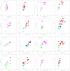 |
Fig. A.1. As in Fig. 5, but for NGC 4590, NGC 4833, NGC 5904, NGC 6093, NGC 6121, NGC 6205, NGC 6254, and NGC 6397. |
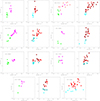 |
Fig. A.2. As in Fig. 5, but for NGC 6535, NGC 6715, NGC 6752, NGC 6809, NGC 6838, NGC 7078, NGC 7099, and NGC 6388. For the last GC, only the relation from our data in the present paper is available. |
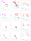 |
Fig. A.3. As in Fig. 6, but for NGC 2808, NGC 3201, NGC 4590, and NGC 4833. |
 |
Fig. A.4. As in Fig. 6, but for NGC 5904, NGC 6093, NGC 6121, and NGC 6205. |
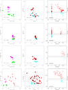 |
Fig. A.5. As in Fig. 6, but for NGC 6254, NGC 6397, NGC 6535, and NGC 6715. |
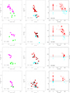 |
Fig. A.6. As in Fig. 6, but for NGC 6752, NGC 6809, NGC 6838, and NGC 7078. |
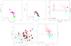 |
Fig. A.7. As in Fig. 6, but for NGC 7099 and NGC 6388. |
Appendix B: Notes on particular stars in a few GCs
In a few plots, some stars are apparently either missing with respect to the numbers given in Table 2 or are in an odd position on the PCMs. In the following, we highlight possible problems related to the identification of stars with spectroscopic abundances from the figures in Marino et al. (2019), and we note particular stars on the PCMs. Flag F indicates stars found and used by Marino et al. (2019), and flag M indicates additional stars found only by us (see Section 2.2).
B.1. NGC 104
Star R0009274 could be a star on the AGB, according to its position in the CMD magF275W, (magF275W-magF814W) (although not when judging from other CMDs).
B.2. NGC 362
Stars R0000796 and R0009389 (both also found in Marino et al. 2019) could be among the so called red-RGB stars, according to the magF336W, (magF336W-magF814W) CMD. To these, we add star R0009282, which was neglected by Marino et al., as a possible red-RGB star.
B.3. NGC 1851
Two stars neglected in Marino et al. (2019; star R0000480 and star R0015479) are located in the region attributed to red-RGB stars, the same as star R0015322, which was used by Marino et al.
B.4. NGC 2808
There is a star in the PCM by Marino et al. (2019) located at about Δcol, Δcol3 = ( − 0.416, 0.175) and classified as FG star (Figure 1 in Marino et al.). We note that this is the object making the sequence of FG stars in NGC 2808 so extended. However, we were unable to find a star located at this value of Δcol3 in their Figure 9, even if all the matches in this GC have an Na abundance. For unknown reasons, this star, plotted on their PCM as having spectroscopic abundances, was then dropped in the Na-Δcol3 relation. Several stars in this GC, both found and neglected in Marino et al. (e.g. stars R0033484, R0027893, R0016679, and R0009902) seem to lie in the saturation region. Star R0005798 (flag=F) and star R0021965 (flag=M) are outside the RGB in the magF336W (magF336W-magF814W), but not in the magF275W (magF275W-magF814W).
B.5. NGC 6121
On the Na-Δcol3 relation derived by us, three stars with flag=M (R0000373, R0000417, and R0000781; [Na/Fe] = 0.05, 0.41, and 0.43) are superimposed to stars R0000301, R0000863, and R0000749 ([Na/Fe] = 0.06, 0.38, and 0.40), flag=F, respectively. Star R0001022 ([Na/Fe] = 0.25) is superimposed to star R0001728 ([Na/Fe] = 0.24), both with flag=F. Judging by its position on the PCM, star R0000101 (flag=F) could be a misidentification on our part. Both the superpositions and the possible misidentification are mostly due to the abundances in Marino et al. (2008) being provided with only two significant decimal figures, so many stars result with the same or a very similar Na and are difficult to assign on the basis of the figures in Marino et al. (2019) alone.
B.6. NGC 6205
In this GC we identified three stars from the figures in Marino et al. (2019) that do not have the complete set of colours to make them appear on the PCM (based on the photometry by Nardiello et al. 2018), even if they are likely matches according to the coordinates. Star R0001523 (L-666, [Na/Fe] = 0.12 in Johnson and Pilachowski 2012) does not have magF336W. Star R0012534 (L-261, [Na/Fe] = 0.06 in Johnson and Pilachowski) does not have magF336W. Star R0002021 (L-324, [Na/Fe] = 0.27 in Johnson and Pilachowski) does not have magF438W. It is unlikely that we misidentified all three; e.g. among the stars matched in coordinates between Nardiello et al. and Johnson and Pilachowski, there is no star with [Na/Fe] = 0.12, such as star L-666=R0001523. When considering both coordinates and Na abundances, we have no explanation on why these objects are located on the PCM used in Marino et al. (2019). Finally, star R0001319 (L-370, [Na/Fe] = 0.27), with flag=F is superimposed to star R0003036 (L = 296, [Na/Fe] = 0.28), with flag=M.
B.7. NGC 6254
Star R0001704 ([Na/Fe]=-0.137, flag=F) is superimposed on star R0001056 ([Na/Fe]=-0.128, flag=M).
B.8. NGC 6715
Star R257062 ([Na/Fe] = 0.587) found by Marino et al. (2019) should not be on a PCM, having no magF814W. Perhaps this is a misidentification in Marino et al. that has been confused for another star.
B.9. NGC 6752
Analogously, star R010792, found in Marino et al. (2019), should not be in a PCM, as it has no magF336W. From the Na-O anti-correlation shown in Figure 8 of Marino et al., this object is unambiguously identified as star NGC 6752-21694 in Carretta et al. (2009a), with [O/Fe], [Na/Fe] = 0.091, 0.318; yet, we were not able to put it on our PCM due to the lack of all required magnitudes. It is unclear how this star can appear among those with both HST photometry and Na abundances in Marino et al. (2019).
All Tables
Stars with Na abundances retrieved in HST photometric catalogues (the complete table is available at the CDS).
Number of mismatches between photometric and spectroscopic classification of MPs.
Pseudo-colour maps (PCMs) for all 22 GCs in the sample. The complete table is only available at the CDS.
List of mismatches between the photometric and spectroscopic classification of MPs.
All Figures
|
Fig. 1. Colour (and pseudo-colour) magnitude diagrams for NGC 104. The upper panels show the CMDs for NGC 104, col versus magF814W and col3 versus magF814W. The red and blue lines are the fiducials used. Lower left panels: rectified RGBs in the normalized col and col3. Lower right panel: resulting PCM, where FG stars are those located below approximately 0.1 in Δcol3 and SG stars above. |
| In the text | |
|
Fig. 2. Comparison of photometric parameters for the group of stars in all GCs with spectroscopy found in Marino et al. (2019; blue crosses) and those added only in the present work (red crosses), as a function of the magnitudes in F814W. The quality and sharpness parameters are from the catalogues of Nardiello et al. (2018) used to construct the PCMs. |
| In the text | |
|
Fig. 3. Distribution of membership parameter from Nardiello et al. (2018) for stars only used by Marino et al. (2019: blue line) and only added in the present work (red line). Upper panel: Histogram of the membership parameters. Lower panel: Cumulative distribution. |
| In the text | |
|
Fig. 4. Examples of saturation effect in col3, F814W plot for three GCs in our sample. Filled black circles are stars with spectroscopy available used by Marino et al. (2019). These stars also lie outside the vertical distribution of the RGB, so we extended the fiducial lines to bracket also these objects. |
| In the text | |
|
Fig. 5. Relations Δcol3–[Na/Fe] for NGC 104, NGC 288, NGC 362, NGC 1851, NGC 2808, and NGC 3201. For each GC, in the left panel the green and magenta symbols mark FG and SG stars, respectively, as classified from HST photometry (through the PCMs). The red triangles represent stars in the so-called red-RGB region. In the right panel, for each GC black circled symbols are stars in common between photometry and spectroscopy, yet they were neglected in Marino et al. Here, FG and SG stars (cyan and red, respectively) are separated according to the spectroscopic Na abundances (see text). |
| In the text | |
|
Fig. 6. Stars with spectroscopy on the PCMs of NGC 0104, NGC 288, NGC 362, and NGC 1851. In the left panels, the photometric classification of MPs is adopted; and in the middle panels, the population assignment is based on spectroscopy. Our PCMs are indicated with small grey dots. In the right panels, stars considered mismatches in classification are superimposed to the Na−O anti-correlation (as filled symbols). Solid lines in each GC indicate the limit [Na/Fe]min + 0.3 dex (with a range ±0.07 dex, dashed lines) used to separate FG and SG stars. The colour-coding is as in Fig. 5. |
| In the text | |
|
Fig. 7. Relation between fraction of mismatches in population tagging and the cluster metallicity. In the left panel, all the mismatches of Table 4 are counted, and the solid line is a linear fit to the data (Pearson correlation coefficient and the two-tail probability are labelled in the panel). In the left panel, fractions are computed using only major mismatches. |
| In the text | |
|
Fig. 8. Comparison of CN (Smith et al. 2013) and Na (Carretta et al. 2009a,b) indicators of MP tagging in NGC 5904 for stars in common between the two studies. The horizontal dashed line separates CN-strong (top) and CN-weak (bottom) stars, whereas blue and red filled circles represent FG and SG stars, respectively, as tagged by our spectroscopic criterion based on Na abundances (see Section 3.1). |
| In the text | |
|
Fig. 9. Same as Fig. 8, but for four more GCs. Upper left panel: 47 Tuc, with CN index from Smith (2015) and O, Na from Cordero et al. (2014). Upper right panel: M 13, with CN index from Smith & Briley (2006) and O, Na from Johnson & Pilachowski (2012). Lower left panel: M 4, with CN index from Smith & Briley (2005) and O, Na from Marino et al. (2008). Lower right panel: NGC 6752, with CN index from Smith (2007) and O, Na from Carretta et al. (2007). |
| In the text | |
|
Fig. 10. Differences, ΔFG, in the fraction of FG stars from HST photometry through the PCMs and from the Na criterion as a function of the fraction of mismatches found in the present paper. A linear fit, with Pearson correlation coefficient and probability is also plotted. |
| In the text | |
|
Fig. 11. Sodium distribution in the three GCs ouliers in Fig. 10 compared to the sample of field stars homogenized in Carretta (2013, triangles). Red, blue, and green filled circles are the P, I, and E components according to Carretta et al. (2009a). The red line reproduces the fraction of FG stars according to Milone et al. (2017) from PCMs (see text). From left to right, the panels are for NGC 288, NGC 2808, and NGC 6838. |
| In the text | |
|
Fig. 12. Differences ΔFG as a function of the total absolute magnitude of the 22 GCs in this study. |
| In the text | |
|
Fig. A.1. As in Fig. 5, but for NGC 4590, NGC 4833, NGC 5904, NGC 6093, NGC 6121, NGC 6205, NGC 6254, and NGC 6397. |
| In the text | |
|
Fig. A.2. As in Fig. 5, but for NGC 6535, NGC 6715, NGC 6752, NGC 6809, NGC 6838, NGC 7078, NGC 7099, and NGC 6388. For the last GC, only the relation from our data in the present paper is available. |
| In the text | |
|
Fig. A.3. As in Fig. 6, but for NGC 2808, NGC 3201, NGC 4590, and NGC 4833. |
| In the text | |
|
Fig. A.4. As in Fig. 6, but for NGC 5904, NGC 6093, NGC 6121, and NGC 6205. |
| In the text | |
|
Fig. A.5. As in Fig. 6, but for NGC 6254, NGC 6397, NGC 6535, and NGC 6715. |
| In the text | |
|
Fig. A.6. As in Fig. 6, but for NGC 6752, NGC 6809, NGC 6838, and NGC 7078. |
| In the text | |
|
Fig. A.7. As in Fig. 6, but for NGC 7099 and NGC 6388. |
| In the text | |
Current usage metrics show cumulative count of Article Views (full-text article views including HTML views, PDF and ePub downloads, according to the available data) and Abstracts Views on Vision4Press platform.
Data correspond to usage on the plateform after 2015. The current usage metrics is available 48-96 hours after online publication and is updated daily on week days.
Initial download of the metrics may take a while.