| Issue |
A&A
Volume 690, October 2024
|
|
|---|---|---|
| Article Number | A354 | |
| Number of page(s) | 13 | |
| Section | The Sun and the Heliosphere | |
| DOI | https://doi.org/10.1051/0004-6361/202348823 | |
| Published online | 22 October 2024 | |
Investigating high-frequency quasi-periodic oscillations in the 6374 Å red coronal line observed during the total solar eclipse on August 21, 2017
1
Shanghai Astronomical Observatory, Chinese Academy of Sciences, Shanghai 200030, China
2
Yunnan Observatories, Chinese Academy of Sciences, Kunming 650011, China
⋆ Corresponding author; This email address is being protected from spambots. You need JavaScript enabled to view it.
Received:
2
December
2023
Accepted:
30
August
2024
Abstract
Context. We present the results of the search for high-frequency quasi-periodic oscillations (HFQPOs) in the 6374-Å red line emission from the solar corona during the 2017 total solar eclipse (TSE).
Aims. The existence of HFQPOs of coronal intensity remains unclear. Motivated by previous observations, this paper focuses on searching for the HFQPOs (> 0.1 Hz) during the 2017 TSE.
Methods. Wavelet analysis tools were used to analyze the radiation intensity oscillations in different height layers, local regions of interest (such as the east coronal loop, west cavity, etc.), and coronal feature points as well as changes in oscillations along coronal feature structures and the kinematic wobble of the coronal magnetic features.
Results. We have observed oscillatory signals at multiple spatial locations, which reveal the existence of quasi-periodic slow magnetoacoustic waves. These signals display periods ranging from approximately 3 to 9 seconds, with a notable focus on periods around 4 seconds.
Conclusions. High-frequency quasi-periodic slow magnetoacoustic oscillations (with periods less than 9.63 seconds) have been identified in the inner corona (at heights less than 1.4 R⊙) in the 6374 Å red coronal line radiation.
Key words: Sun: corona / Sun: oscillations
© The Authors 2024
 Open Access article, published by EDP Sciences, under the terms of the Creative Commons Attribution License (https://creativecommons.org/licenses/by/4.0), which permits unrestricted use, distribution, and reproduction in any medium, provided the original work is properly cited.
This article is published in open access under the Subscribe to Open model. This email address is being protected from spambots. You need JavaScript enabled to view it. to support open access publication.
1. Introduction
To date, the cause of coronal heating is not entirely clear, and efforts to determine the dominant heating mechanism have yielded two of the most widely accepted candidates: a direct current (DC) type and an alternating current (AC) type (Williams et al. 2001; Rudawy et al. 2019). The DC mechanism is based on numerous small reconnections of the highly filamentary coronal magnetic field, which is referred to as the flare or nanoflare heating model originally proposed by Parker (Parker 1988). It is thought that after countless magnetic reconnections in the form of flare and nanoflare activity throughout the corona, the corona is heated by current dissipation (Levine 1974; Parker 1988; Pontin & Hornig 2015; Pontin et al. 2017; Samanta et al. 2019; Bi et al. 2023). In the AC category, heating is driven by the attenuation of magnetohydrodynamic (MHD) waves propagating from the lower solar atmosphere and dissipating through ion viscosity and electrical resistivity (Hollweg 1982; Williams et al. 2001; De Moortel & Nakariakov 2012; Matsumoto 2018; Rudawy et al. 2019). In this paper, we investigate the high-frequency quasi-periodic oscillations (HFQPOs; the oscillation period less than 10 seconds is mainly analyzed in this work) during a total solar eclipse (TSE) under the AC strategy.
The typical periods of the coronal waves and oscillations are in the range of a few seconds up to a few minutes (Nakariakov & Verwichte 2005). Theoretical work has shown that high-frequency MHD waves (with frequencies > 1 Hz) could effectively transport energy into the solar corona (Porter et al. 1994). In other words, coronal oscillations, especially short-period intensity oscillations and traveling waves, may be important for energy transport from the lower atmosphere to the corona. This is especially true for quiet regions such as the plume feathers, where the open magnetic fields and magnetic reconnections cause particle acceleration rather than heating of the plasma volume (Rudawy et al. 2004). Therefore, the detection of coronal HFQPOs is important for understanding the coronal heating problem.
Although ground-based coronagraphs and telescopes on board satellites do a good job of covering many areas of coronal research, it must be admitted that there are still some areas of coronal research that can only be observed from Earth during a TSE. For example, for the detection of high temporal resolution coronal oscillation signals, TSE provide rare optimal opportunities to improve our understanding of the solar corona. Coronal data are typically too weak, have a poor signal-to-noise ratio (S/N), and lack high-frequency information. Long exposures are often required to improve the S/N, making it nearly impossible to study high-frequency oscillations. Imaging cadences from spacecraft, even from the Atmospheric Imaging Assembly (AIA) on board the Solar Dynamics Observatory, are still insufficient to search for such periods (with MHD wave frequencies > 0.5 Hz) (Rudawy et al. 2010; Pesnell et al. 2012). During a TSE, radiation from the photosphere and chromosphere is blocked by the Moon, so most of the “stray light” introduced by the lower atmosphere is removed, allowing one to observe the coronal signal with a high S/N and temporal resolution. The detection of coronal HFQPOs during a TSE has unique advantages. The dissipated energy can give rise to periodic or quasi-periodic intensity oscillations, especially in coronal visible emission lines such as the green line (Fe XIV 530.3 nm) or the red line (Fe X 637.4 nm) (Rudawy et al. 2019).
Over the past few decades, several attempts have been made to detect evidence of HFQPOs, but consensus on the results is yet to be reached. Some studies suggest that there are no significant coronal intensity oscillation signals. However, there are also results suggesting that there are clear oscillations in the intensity of the corona. Koutchmy et al. (1983), using coronagraphic observations, found evidence for Doppler velocity oscillations with periods close to 300 seconds, 80 seconds, and especially 43 seconds, but there were no prominent intensity variations. Pasachoff & Landman (1984) detected excess power in Fourier transforms of the data for the region between 0.5 and 2 Hz at the level of one or two of the incident power during the 1980 eclipse, and the weak periodic modulations of the intensity of the coronal Fe XIV green line (5303 Å) were reported. During the 1983 eclipse, Pasachoff & Ladd (1987) confirmed the above results indicating the presence of excess power in the coronal green line radiation in the frequency range 0.25–2.0 Hz, especially in the range 0.25–0.50 Hz. Variations of the continuum intensity with periods in the range of 5–56 seconds were detected by Singh et al. (1997) during the TSE of October 24, 1995. These oscillations have been found to be sinusoidal, and their amplitudes have been found to be in the range of 0.2–1.3% of the coronal brightness. A least squares analysis yielded periods of 90.1, 25.2, and 6.9 seconds for the three prominent components during the TSE of February 26, 1998, reported by Cowsik et al. (1999). A Monte Carlo model was used for the data obtained during the August 11, 1999, TSE by Pasachoff et al. (2002), and the authors suggest that the presence of enhanced power, particularly in the range 0.75–1.0 Hz, and the MHD waves remain a viable candidate for coronal heating. It is puzzling that when analyzing the observations of the TSEs of November 3, 1994, in Putre, Chile, and February 26, 1998, in Nord, Aruba, Pasachoff et al. (2000) did not consider them as definitive evidence of coronal oscillations at high frequencies of the coronal green line brightness. The Solar Eclipse Coronal Imaging System (SECIS) (Phillips et al. 2000), as a unique instrument designed to search for short-period modulations in the solar corona during a total eclipse, has been used for several TSE observations. On August 11, 1999, during the 2 minutes and 23.5 seconds of the TSE, the SECIS experiment produced initial findings, including the identification of quasi-periodic disturbances lasting 6 seconds, which were observed propagating along a coronal loop (Williams et al. 2001, 2002; Cooper et al. 2003). However, by using classical Fourier spectral analysis tools, Rudawy et al. (2004) examined temporal variations of the local 530.3 nm coronal line brightness in the 1–10 Hz frequency range, and they found no clear and statistically significant evidence of periodicities at any of the points examined. During the TSE of March 29, 2006, significant intensity oscillations (about 27 seconds for the green line and 20 seconds for the red line) with high probability estimates were detected at the boundary of an active region and in its neighborhood by Singh et al. (2009). An improved Fe XIV green line (5303 Å) dataset obtained during the 2001 TSE observed from Zambia was analyzed by Rudawy et al. (2010), but no statistically significant period in the range 0.06–10 Hz was found. In the recent TSE of 2017, no statistically significant HFQPOs were found either (Rudawy et al. 2019). In recent years, significant advancements have been made in the study of high-frequency decayless waves in similar locations, facilitated by the launch of the Extreme Ultraviolet Imager on board the Solar Orbiter (SO/EUI) instrument (Rochus et al. 2020). These studies have also detected similar oscillation periods, further confirming the reliability and scientific significance of the HFQPO results. Using SO/EUI, Petrova et al. (2023) detected transverse oscillations with periods of 14 s in a 4.5 Mm loop and 30 s in an 11 Mm loop. Lim et al. (2023) identified power-law relationships in the distribution of energy flux and oscillation count relative to energy in their investigation. The power-law slope (δ = −1.40) of the energy flux versus frequency suggests that high-frequency oscillations may dominate the overall heating process (δ < 1). Additionally, the power-law slope (α = 1.00) of the oscillation count versus energy flux indicates that oscillations with a higher energy flux contribute significantly to the total heating. These results underscore the potential importance of high-frequency oscillations in coronal heating through undamped transverse oscillations. In another recent study, Shrivastav et al. (2024) analyzed 42 oscillations in coronal loops ranging from 3 to 23 Mm in length. They reported an average displacement amplitude of 134 km, oscillation periods ranging from 28 to 272 seconds, and velocity amplitudes between 2.1 and 16.4 km/s. They also noted that short-period decayless oscillations are not commonly found in the quiet Sun and coronal holes. In conclusion, oscillations with periodicities of a few seconds are not always successfully observed. This can be attributed to various factors, such as the time of day an observation is made, the specific solar region being studied, the level of solar activity at the time, and limitations in the instrumental performance. All of these elements can contribute to the absence or difficulty in detecting these short-period oscillations in certain observations.
Motivated by the previous observations, this paper reports on a search for HFQPOs of the Fe X 6374 Å coronal red emission line during the August 21, 2017, TSE. The rest of this article is as follows. Section 2 reviews the basic information about the 2017 TSE observations. Section 3 describes the data reduction process. Section 4 presents the results of the wavelet analysis of the HFQPOs. A discussion and conclusions are given in the last section.
2. Observations and instrumentation
The instruments were set up on a flat grassy meadow located on a farm outside of Oregon (N44° 55′, W123° 18′) within the band of totality. The sky over the observation site was clear during the TSE. The totality started at 17:16:57 UT on August 21, 2017, and lasted approximately 108 seconds. For the analysis of high-frequency coronal oscillations, we selected approximately 25.35 seconds (56 frames) of data. This selection was necessary because the first part of the eclipse duration (from 17:16:57 UT to 17:18:16 UT, approximately 80 seconds) was dedicated to polarization observations. Additionally, about 3 seconds of data starting after 17:18:41 UT were discarded due to significant fluctuations in coronal brightness, which impeded the precise registration of coronal features. Consequently, only the data from 17:18:16.164 to 17:18:41.514 (approximately 25.35 seconds) were usable for searching for HFQPOs. According to the Nyquist law of sampling, the sampling method is capable of detecting oscillatory signals with periods shorter than 12.675 seconds. A 152 mm aperture, f/10 refracting telescope is used for TSE observation. The observations utilized a 5 Å full width at half maximum (FWHM) bandpass custom “DAYSTAR1” filter, which was centered at the coronal red line of Fe X at 6374 Å. The filter was equipped with a temperature control system to ensure the stability of the bandpass center frequency within the observed spectral band. Images of the corona were taken with a Baumer LXC-250M sCMOS 16-bit monochrome camera consisting of 5120 × 5120 square pixels with dimensions of 4.5 μm2. During the whole observation, an automatic tracking program was used. The tracking speed of the equatorial mount was set to the speed of the Sun.
Figure 1 presents the Fe X 6374-Å coronal red line image observed during the totality and the corresponding SDO/AIA (Pesnell et al. 2012) composite data. In the left panel, the Fe X 6374-Å red line image is shown, while the right panel provides the RGB pseudo SDO/AIA data, which is composited by R (211 Å), G (193 Å) and B (171 Å). As can be seen in the figure, coronal features in the Fe X 6374-Å above the solar limb are in good agreement with the SDO/AIA data. The structures, such as the plumes in the polar regions, are clearer and more pronounced in the Fe X 6374-Å than in the SDO/AIA extreme ultraviolet (EUV) data. This may be because in the coronal cavity region, Fe X radiation, which represents low temperatures, has a larger fraction of radiation than high temperature plasma.
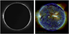 |
Fig. 1. Overview of coronal states during the August 21, 2017 TSE. Left panel: Coronal image of Fe X 6374-Å observed at 17:18:16.570 UT during the August 21, 2017, TSE. Right panel: SDO/AIA RGB composite image on August 21, 2017. The red channel represents the 211 Å data observed at 17:09:33 UT, the green channel denotes the 193 Å data observed at 17:11:40 UT, and the blue channel is the 171 Å data observed at 17:12:09 UT. The 6374-Å and the SDO/AIA composite coronal images have both been rotated so that the vertical axis is in the north-south direction. |
3. Data processing
3.1. Preprocessing
The first step in our data processing was dark current subtraction and flat-field preprocessing. Within an hour after the totality, we maintained the instrument in the same state as the TSE observation and immediately collected 24 frames of flat-field data. The flat-field data covered multiple pointing regions, with varying right ascension (RA) and declination (Dec) angles. The weather conditions were favorable, with clear skies and no wind during data acquisition. The dark current data were collected in the laboratory. To obtain coronal oscillation information from the time series coronal image, rigorous preprocessing was required, including dark field removal, flat-field correction, and time series image registration.
3.2. Coronal images registration
Although the equatorial telescope mount was used for automatic tracking during totality, the pointing showed small errors due to factors such as wind loading and tracking error. The main cause is the slow drift caused by the drive axis adjustment error, which manifests itself as a small drift (pixel level) of the time series image. Therefore, image registration must be applied for subsequent photometric analysis and intensity oscillation detection. Coronal images typically have a low S/N ratio, a high dynamic range, and a lack of high-frequency feature information. Rigorous registration of coronal images is not an easy task, as discussed in our previous paper (Liang et al. 2021). We present the following approach for image registration: The cross-correlation (CC) algorithm was used for image registration. The principle of the CC method is outlined as follows (Zitová & Flusser 2003; Yoo & Han 2009):
 (1)
(1)
where f and g respectively represent the sensed and reference images; x, y are the position of the pixel; and μ and δ are the mean values of the image and the standard deviation of the image. The term γ(f,g) represents the correlation coefficient, which is based on statistics to calculate the correlation between two sets of sample data, and its value ranges from [−1, 1]. For image registration, a sub-pixel image registration from the CC algorithm2 (Guizar-Sicairos et al. 2008) was used. In this paper, in a multi-frame image of a time series, we used a first frame image as a reference frame g, and the subsequent frames were cross-correlated with the first frame to calculate their offsets, and then the calculated offsets were used to perform the image registration. The process consisted of three main steps.
-
Preliminary registration using the lunar limb: The initial step involved utilizing the high S/N ratio characteristics of the lunar limb for preliminary registration, aimed at compensating for excessive image drift errors. In this step, the entire field of view (FOV) of the lunar limb, as represented in the left panel of Fig. 2, was employed as the alignment reference.
Fig. 2. Reference field of view and feature regions for coronal registration. Left panel: Complete FOV of the lunar limb utilized for the initial image registration. This image was captured at 17:18:57.402 UT during the TSE on August 21, 2017. Right panel: Magnified view of the area indicated in the left panel, which is employed for subsequent image registration processes.
-
Accurate calculation of image shift values: In the second step, the prominence feature indicated by the red box in the left panel of Fig. 2 was utilized to accurately calculate the image shift values.
-
Rigorous registration of coronal images: Finally, a rigorous coronal image registration was executed using the offsets determined in the previous steps.
3.3. Wavelet analysis
To search the HFQPO signals, we employed wavelet methods to perform the data analysis. The Difference of Gaussian (DOG) mother wavelet was used for wavelet diagnosis, and the data were normalized before wavelet diagnosis. Among the common wavelet basis choices used in practice, the Morlet, DOG, and Meyer wavelets are frequently employed for time-domain signal analysis. For our particular dataset, the DOG wavelet performs better at detecting sudden changes. This is because the DOG wavelet is particularly sensitive to abrupt and local features, which is essential for detecting the transient appearance of coronal high-frequency oscillations.
In this paper, to make data with different intensity values comparable after wavelet analysis, the data were de-trended and then normalized using their own standard deviations (except for spatial shift analysis in Section 4.1). The algorithm used to de-trend and normalize the input data is as follows: First, a first-degree polynomial fit was applied to remove the linear trend from the data. Then, the standard deviation of the de-trended data was calculated, and normalization was achieved by dividing the data by this standard deviation.
4. Data analysis
4.1. Stability and coalignment of the coronal images
Due to the influence of such aspects as tracking error, wind load, and seeing, which introduce small-scale pointing errors, fine-tuning was required to achieve accurate registration of the time series images so that wavelet analysis could then be applied. As discussed in Section 3.2, the lunar limb and the bright structure of the corona were used sequentially for image registration. However, it should be noted that accurate registration of coronal images is not easy, and it is difficult to achieve more ideally accurate (sub-pixel) registration results. This method is sensitive to the referenced coronal bright structure, and ultimately the judgment criterion is whether the time domain variation of the detailed features of the corona is reasonable.
Figure 3 illustrates the tracking offsets of the solar corona observed during the TSE. These offsets were calculated through a two-step image registration process: an initial alignment based on the Moon’s limb followed by a precise alignment using the prominence features. The top panels of Fig. 3 list the X and Y axis shift values diagnosed by the image registration process, while the wavelet analysis results are shown in the corresponding bottom panels. As shown in Fig. 3(a), the spatial drift of the X-axis is nearly linear, with a spatial amplitude of about 12 pixels (54 μm) in the focal plane of the detector, while a small drift is present in the Y-axis, with an amplitude of about 5 pixels (22.5 μm). To analyze the frequency domain characteristics, we conducted wavelet analyses on the shifts in the x-axis and y-axis. The results are shown in Fig. 3 (b) and (c). Taking Fig. 3(b) as an example, the left side of the figure presents the wavelet scalogram, where the x-axis represents time, the y-axis represents scale (corresponding to frequency), and the color intensity indicates the magnitude of the wavelet coefficients. This diagram reveals the temporal localization of frequency components, highlighting transient features and non-stationary behaviors. High-frequency components are concentrated at specific times, indicating transient events or abrupt changes. The cone of influence (COI) in wavelet analysis stems from boundary effects of the signal and the localization properties of wavelet basis functions, leading to potentially unreliable results near the signal edges. To ensure accuracy, data outside the COI should either be excluded or processed using appropriate boundary handling methods. In this study, shaded areas outside the COI represent regions of low confidence, while highlighted areas denote regions of high confidence, as depicted in Figures (b) and (c). Specifically, the analysis excludes results from the COI (shaded region). Furthermore, all wavelet analyses in this paper employed a global transform approach to analyze the entire signal across all scales, encompassing 56 frames over a duration of 25.35 seconds. The right panel of Fig. 3(b) depicts the power spectrum of the signal, where the X-axis denotes signal power and the Y-axis represents frequency. This spectrum illustrates the energy distribution across frequencies, facilitating the identification of dominant frequencies, with a dotted line indicating the 95% confidence level. Integrating the wavelet spectrogram with the power spectrum offered a comprehensive understanding of the time-frequency characteristics of the signal. The wavelet spectrogram provides temporal localization of frequencies, while the power spectrum offers a global frequency distribution, enabling robust analysis of complex, non-stationary signals.
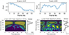 |
Fig. 3. Spatial shift values and their wavelet analysis results. The upper panels present the shift values for both axes observed during the totality. The lower panels depict the corresponding wavelet analysis results for these displacements. |
The results of the wavelet analysis for the X-axis, Y-axis shift data demonstrate that the spatial drift on the X-axis is characteristic of oscillations that have no more than 95% confidence, while the Y-axis has oscillation characteristics with a period with a peak frequency around 14.4 seconds, which may be related to the non-linearity fluctuation of the spatial drift of the Y-axis. But this is beyond the limits of the sampling frequency, and therefore the periodic signal is unreliable. We concluded that image drifts caused by telescope tracking and other factors do not show periodic oscillations smaller than 12.675 seconds. Furthermore, the effect of image registration correction mitigates this impact. This was achieved by conducting subsequent analyses after calibrating these spatial displacements through image registration.
4.2. Search for the intensity HFQPOs in the lunar background
After correcting the tracking error, accurately calculated through image registration, we analyzed the intensity fluctuations of the moon’s background by averaging the intensity over the entire lunar surface. During totality, the lunar background radiation, which represents the scattering of the coronal brightness, may reflect its changes. The lunar background intensity oscillations of the 56 frames (about 25.35 seconds) selected in this paper are shown Fig. 4. The left panel shows the intensity oscillations of the lunar background, while the right panel provides their wavelet analysis result. It should be noted that the intensity of the lunar background is defined as the average of the entire FOV smaller than the solar radius, and that the range of the intensity fluctuation is 8 × 10⁻⁴. As is shown, an intensity oscillation period between 6 seconds and 16 seconds with a peak value of about 9.63 seconds was detected. Another signal peaks at 28.8 seconds, which is negligible beyond the Nyquist sampling theorem. The total sampling time is about 25.35 seconds, so theoretically the longest period that can be detected for an oscillating signal is 12.675 seconds. In the remainder of this article, only the oscillations with a period less than 12.675 seconds are analyzed.
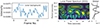 |
Fig. 4. Lunar background intensity during totality and wavelet analysis results. Left panel: Average intensity of the lunar background during the totality. Right panel: Wavelet results of the lunar background intensity. |
4.3. Search for the intensity HFQPOs along the coronal height
We conducted a search for HFQPOs in order to detect the HFQPO signals along the coronal height. The left panel of Fig. 5 shows an image of the coronal polar coordinates, and the right panel lists the layer images. Due to the constraints imposed by the detector’s FOV, this study concentrates on the lower coronal region at a radial height below 1.8 R⊙.
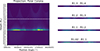 |
Fig. 5. Coronal features in polar form during the August 21, 2017 TSE. Left panel: Coronal intensity along the position angle and the coronal height. Right panel: Layered images as indicated by the corresponding labels. |
The diagnostic results for the fluctuating coronal atmosphere in different layers are shown in Fig. 6. The wavelet analysis results mentioned here refer to the mean value of the intensity signal fluctuating with time within the specified FOV. For comparison, the lunar background intensity results are listed in the lower right panel of Fig. 6, which shows that there is an oscillatory signal with a peak period of 9.63 seconds. As shown in the figure:
-
The wavelet analysis result in the FOV 1.02 R⊙ − 1.05 R⊙ shows that there are hardly any oscillating signals with more than 95% confidence in periods shorter than 12 seconds. The same result applies for the range of 1.05 R⊙ − 1.1 R⊙. But the wavelet analysis of the combination of the above two FOVs (1.02 R⊙ − 1.1 R⊙) shows that there are oscillating signals with more than 95% confidence in a period of about 10 seconds. It is not clear what the cause of this problem is. A possible reason is that the signal is not strong enough for the oscillation to appear in the two bands, but when they are combined together, the signal becomes sufficient.
-
The wavelet analysis result in the FOV 1.1 R⊙ − 1.2 R⊙ shows that there are hardly any oscillating signals with more than 95% confidence in periods shorter than 12 seconds.
-
The wavelet analysis result in the FOV 1.2 R⊙ − 1.3 R⊙ shows that there is an oscillation signal with a period of 5 and 10 seconds (with more than 95% confidence). A similar result applies for the range 1.3 R⊙ − 1.4 R⊙.
-
The wavelet analysis of the entire FOV (1.02 R⊙ − 1.8 R⊙) shows that there are oscillating signals with more than 95% confidence in a period of about 8.6 seconds.
For the oscillation signal of around 9.63 seconds, it may be affected by the combination of instruments, weather, seeing, and other factors since the observation of no radiation source in the lunar background shows the existence of oscillations in that period. However, the HFQPOs of about 5 seconds give us reason to believe that there are high-frequency intensity oscillations in the coronal plasma radiation in the range of 1.2 R⊙ − 1.4 R⊙.
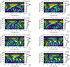 |
Fig. 6. Wavelet analysis of high-frequency signals along the coronal height. The figure comprises several panels illustrating the wavelet analysis of intensity fluctuations across different segments of the coronal height. Each panel represents a distinct region and the corresponding range of intensity fluctuations. Panel (a) presents wavelet analysis of the intensity form R1.02 to 1.05, the range of the intensity fluctuation in 5 × 10⁻³. Panel (b) covers the range R1.05 to R1.1, where the intensity fluctuation is measured at 2 × 10⁻³. Panel (c) encompasses a broader range, from R1.02 to R1.1, with a fluctuation scope of 1.6 × 10⁻³. Panel (d) extends from R1.1 to R1.2, detailing intensity fluctuations of 6 × 10⁻⁴. Panel (e) spans from R1.2 to R1.3, where intensity fluctuations are observed at 5 × 10⁻⁴. Panel (f) illustrates the region from R1.3 to R1.4, recording intensity fluctuations of 4 × 10⁻⁴. Panel (g) demonstrates a larger range from R1.02 to R1.8, with a noted intensity fluctuation of 2 × 10⁻⁴. Panel (h) presents the wavelet analysis against a lunar background, indicating intensity fluctuations of 8 × 10⁻⁴. |
4.4. Search for the intensity HFQPOs in the regions of interest
To verify that the oscillation factors in the range of 1.2 − 1.4 R⊙ are larger than those in the range of 1.02 − 1.2 R⊙, several coronal feature regions were captured for comparative analysis. We note that to make the results more reasonable, we used the range 1.2 − 1.38 R⊙ instead of 1.2 − 1.4 R⊙ to be consistent with the spatial region size of 1.02 − 1.2 R⊙. A total of five representative coronal regions were selected for comparative analysis: the coronal loop where the active region is located, the coronal dark activity, the prominence, the polar plume, and the coronal hole. It is worth investigating what the specific source of the intensity oscillation is, and to achieve this goal, we studied several groups of coronal plasma structures through wavelet analysis. The wavelet analysis results of the mean intensity of the five representative coronal regions are shown in Fig. 7. The panels in the left column show the intensity maps of the five selected regions for wavelet analysis in the height range from 1.02 to 1.2 R⊙, while the second column on the left shows the corresponding intensity maps in the range from 1.2 to 1.38 R⊙. The panels in the third column show the wavelet analysis results of the mean intensity of the five selected regions in the spatial range of 1.02 − 1.2 R⊙, and the corresponding rightmost column shows the wavelet analysis results of 1.2 − 1.38 R⊙. As shown in the figure, “PA” represents the clockwise position angle according to a polar coordinate model for images, starting at 0 degrees from the north pole, going to 90 degrees west, 180 degrees south, 270 degrees east, and then returning to 360 degrees (0 degrees) north.
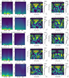 |
Fig. 7. Wavelet analysis of high-frequency signals in the regions of interest. |
-
In the eastern coronal loop region (PA 260° −280°), which represents the active region, there are almost no intensity oscillation signals with 95% confidence. Although the radiation intensity and magnetic field near the active region are relatively strong, the results indicate that the radiation in this region is relatively stable, and there are few oscillations.
-
In the western coronal cavity region (PA 85° −105°), no oscillation signal was detected in the average intensity for radial heights below 1.2 R⊙. However, a quasi-periodic oscillation signal with a period of approximately 5 seconds was observed in the radial height range of 1.2 − 1.38 R⊙.
-
In the northwestern prominence region (PA 32° −52°), there are also almost no intensity oscillation signals with 95% confidence. In the 1.2 − 1.38 R⊙ height region, the oscillation signal is stronger than in the lower (1.02 − 1.2 R⊙) region, with a period longer than 10.6 seconds, exceeding the 95% confidence level.
-
In the southern plume region (PA 170° −190°), a quasi-periodic oscillation signal with a peak of about 5 seconds was detected both in the region below 1.2 R⊙ and in the 1.2 − 1.38 R⊙ region. The power spectrum of oscillating signals above 1.2 R⊙ is larger than below.
-
In the northern coronal hole region (PA 340° −360°), a quasi-periodic oscillation signal with a peak of 5.62 seconds was detected below the height of 1.2 R⊙, while a peak of 6.69 seconds was detected above the height of 1.2 R⊙.
In summary, oscillation signals with heights greater than 1.2R are stronger than those in regions below 1.2R, and oscillation signals in regions corresponding to weak magnetic fields (such as coronal cavity, polar coronal hole, polar plum) are stronger than those in regions with strong magnetic fields (such as coronal loop, progress).
4.5. Search for the intensity HFQPOs in potential source points
To locate the source of the intensity oscillations, we performed a wavelet analysis of the time series intensity for a number of coronal feature points. The selected multiple feature points are marked in the left column of Fig. 7. The selection criteria are different for each feature region. In the eastern coronal loop region, one coronal feature point along the closed flux rope and one along the open flux rope were selected to analyze the coherence between the two flux ropes. These points are labeled as point 1 and point 2 in the figure. For the western coronal cavity region, the bright core inside the coronal cavity and another spatial point inside the cavity were used for comparative analysis in order to check the consistency of their internal physical properties. These two points are marked as points 3 and 4. For the northwestern prominences, the bright core points of two different prominences were selected for a comparative analysis of the consistency of the intensity oscillations, marked as points 5 and 6. For the southern polar coronal plume region, a comparative analysis of the consistency of the intensity oscillations between the plume and the interplume spatial points was analyzed. These two points are marked as points 7 and 8. In the northern polar coronal hole region, one spatial point within the coronal interplume was selected to analyze the intensity oscillation characteristics of the coronal interplume region, marked as point 9. The wavelet analysis results for these nine points are shown in Fig. 8. As shown in the figure:
-
No high-frequency oscillation signals with a period of less than 8 seconds were detected in either the open or closed magnetic flux rope areas. This means that strong radiation oscillations are unlikely to exist near areas with strong magnetic fields.
-
In the coronal cavity region, there is a high-frequency oscillation with a period of about 4 seconds in the bright kernel.
-
No intensity oscillation signals were detected in the two prominence regions.
-
In the southern coronal plume region, an oscillation signal with a peak of 5.3 seconds was detected in the plume region (point 7), and its power spectrum intensity exceeded that of the bright kernel (point 3) in the coronal cavity region. No oscillation signal was detected in the interplume region.
-
It is puzzling, however, that while the southern interplume at point 8 showed no intensity oscillation, the northern interplume at point 9 showed an intensity oscillation signal with a peak of less than 6.69 seconds.
The oscillation signals have periods approximately ranging from 4 to 5 seconds.
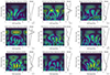 |
Fig. 8. Wavelet analysis results for points 1 through 9. The results are systematically presented, arranged from left to right and top to bottom. |
4.6. Search for the intensity HFQPOs along the characteristic path of the corona
Several representative coronal features listed below were selected to analyze the changes in intensity oscillation signals along their paths. As is marked in the Fig. 9, the features are open magnetic flux rope, closed magnetic flux rope, bright kernel inside the coronal cavity, the magnetic flux surrounding the coronal cavity, plume along the height, and the interplume along the height. In the left panel of Fig. 9, seven points along the open magnetic flux rope are marked as red stars, and another seven white Y-shaped symbols mark the points along the closed magnetic flux rope. In the middle panel of Fig. 9, seven magenta diamonds mark the path along the bright kernel within the coronal cavity, while the black dots mark the contour of the coronal cavity magnetic flux as it rises in height. In the right panel of Fig. 9, seven gold plus signs mark the characteristics of the coronal plume at different heights, while seven purple ‘x’ symbols mark the characteristics of the coronal interplume at different heights. A total of six paths were selected, and seven feature points on each path were selected for wavelet analysis. The results of the wavelet analysis are shown in Table 1. The order of the seven feature points on each path is spatially arranged from low to high for easy comparison. In Table 1, the intensity oscillation peaks detected with a confidence level greater than 95% are highlighted in bold black. Meanwhile, in Fig. 9, the periodic value of HFQPOs is marked near the feature points detected with a confidence level greater than 95%. In the wavelet analysis results:
Peaks of the HFQPOs at each selected point.
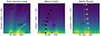 |
Fig. 9. High-frequency quasi-periodic oscillations observed along the inner coronal characteristic structures. Paths are denoted as follows: Path 1 (red stars) and Path 2 (white ‘Y’); Path 3 (magenta diamonds) and Path 4 (black dots); and Path 5 (violet ‘x’) and Path 6 (gold plus signs). |
-
The distribution of the peaks of the detectable periodicity of the HFQPOs signal is usually in the range of 3–5 seconds. This indicates that the 3–5-second quasi-period is not random, although many of the data points do not reach a 95% confidence level. Fig. 10 shows the results of the wavelet analysis for a total of 42 sample points from six characteristic paths of the corona. Seven data points were sampled at intervals ranging from low to high along the coronal features on each path. As shown in Fig. 10 and Table 1, the detectable quasi-periodic signals are mainly concentrated in the range of 3–10 seconds, but when considered with weighting factors exceeding 95% confidence, the quasi-periodic oscillations of 3–5 seconds are more confident.
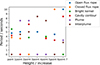
Fig. 10. Scatter of the wavelet analysis results along characteristic paths of the corona. The wavelet analysis quasi-periodic peak scatter plots for all feature points on the six selected paths are shown in this figure. The X-axis represents the height from the bottom layer of the corona along the path. We note that each of the six paths has seven sample points, and their heights on the X-axis may not be consistent. In this figure, we have plotted the heights of the seven sample points together for comparison. The Y-axis represents the quasi-periodic peak value; a period value of zero indicates that the quasi-periodic peak was not detected at the sample point.
-
Along the open magnetic flux rope, the closed magnetic flux rope, the contour of the coronal cavity, and the bright kernel inside the coronal cavity, HFQPO signals of intensity in the range of 3–5 seconds were detected at some spatial points, but most spatial points were not detected.
-
A 10.02-second oscillation signal was detected at the top of the closed magnetic flux rope. On the path of the cavity contour, a 6.69-second period of intensity oscillation signal was detected in a spatial point. On the path of the interplume, a 7.5-second period of intensity oscillation signal was detected in a spatial point.
The spatial points with intensity oscillation signals exceeding 95% confidence are not distributed along the coronal features. The presence of oscillation signals with periods of 3–5 seconds at multiple sampling points seems to indicate that this is not a random phenomenon. The period peaks of the main detected radiation intensity oscillations are distributed in the interval of 3–9 seconds. A similar finding was presented by Katsiyannis et al. (2003), who identified 20 4 × 4 arcsec2 regions showing intensity oscillations in the frequency range of 0.15–0.25 Hz. This observation suggests that these oscillations occur within low emission-measure or different temperature loops associated with the active region.
4.7. Looking for the wobble of the coronal magnetic features
The above subsections all focus on finding the oscillations with a fixed point or region. In this section, the wobble of the coronal magnetic features is examined. As shown in Fig. 11, this study examines the strong magnetic field characteristics of the coronal loop region in the eastern section of the solar active region as well as the western coronal cavity, northwestern prominences, southern plumes, and northern coronal hole regions. To study the wobble of the magnetic flux rope at the core, ten time slices of paths of data from the coronal features region were analyzed. Calculating the center of mass of each slice sample using the radiation intensity as a weight enables the calculation of radiation oscillation along the path. Therefore, by analyzing the pixel index of a slice sample, it is possible to determine the radiation intensity centroid’s oscillation along the path over time. As the magnetic field and matter in the corona are tightly coupled, analyzing the oscillations of the center of radiant intensity over time using wavelet analysis enables the investigation of high-frequency oscillations in the coronal magnetic field structure. Consequently, this analysis facilitates the exploration of HFQPOs.
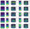 |
Fig. 11. Wavelet analysis results of the wobble of coronal magnetic features. The pixel orientation of the time slice map is from bottom to top and left to right. |
In Fig. 11, the five rows delineate the outcomes of the analysis on the eastern coronal loops, western coronal cavities, northwestern coronal crests, southern coronal columns, and northern coronal holes, sequentially. The first column illustrates the region of interest (ROI) encompassing the coronal features, with the red and white lines indicating the locations of where the samples were collected along the slices. To maintain consistency and reduce uncertainties in the sample slices, the values of four pixels to the left and right of the slice paths were combined, resulting in each slice being nine pixels wide. The second and fourth columns present the temporal slice plots for the respective ordinal samples. The third and fifth columns exhibit the outcomes of wavelet analysis conducted on the center of the radiation intensity over time for the corresponding ordinal time slice plots.
-
In the eastern coronal loop region, slicer 1 is positioned along the open magnetic flux rope, while slicer 2 is oriented across the closed magnetic flux rope. The wavelet analysis findings indicate that no kinematic oscillations are present in the open magnetic flux rope. However, within the closed magnetic flux rope, high-frequency oscillations with period peaks of approximately 4.0 seconds and 7.2 seconds are observed. Radiation intensity wobbles in pixel units can be determined using a center-of-mass algorithm based on radiation intensity data at each time point. Based on the pixel area associated with the lunar profile, the extent of the TSE, and the size of the Sun, the physical size of each pixel in polar form is estimated to be approximately 375 kilometers. This method can be used to calculate both the sub-pixel values and the corresponding physical distances. The amplitude of the oscillation in the radiation intensity centroid is approximately 0.375 pixels, corresponding to 140 km.
-
In the western cavity region, slicer 3 is positioned along the bright kernel inside the cavity, while slicer 4 is oriented across the bright kernel. The wavelet analysis findings indicate that almost no kinematic oscillations are present along the bright kernel. However, across the bright kernel, a high-frequency oscillation with a period peak of approximately 3.6 seconds was detected. The amplitude of the radiation intensity centroid’s oscillation is about 0.4 pixels, corresponding to 150 km.
-
In the northwestern prominences, southern plumes, and northern coronal hole regions, almost no kinematic oscillations are present, except for a peak period of approximately 9.63 seconds detected at slicer 9. However, it should be noted that this period is precisely aligned with the oscillation period of the fluctuations in the radiative intensity of the lunar background, as discussed in Section 4.2. Essentially, this is a pseudo-signal stemming from the lunar background undulations.
In summary, no kinematic oscillation signals were detected along the radial magnetic line direction. However, high-frequency kinematic oscillations are observed in the direction of magnetic line shear, particularly within the coronal closed flux loop and the cavity kernel region. These oscillations have periods of approximately 3.6, 4.0, and 7.2 seconds, consistent with the findings of previous studies that reported oscillation signals with periods of 3–9 seconds at multiple sampling points. Unlike previous analyses focusing on the intensity of coronal radiation oscillations at specific locations or regions, in this chapter we examined the kinematic variations in the magnetic field structure of the corona. It is worth noting that the two oscillations may originate from the same source at the same location, but they represent different manifestations of coronal oscillations in terms of radiative intensity and motion fluctuations.
5. Discussion and conclusions
In this paper, we have investigated the detection of the HFQPOs of the Fe X 6374 Å red coronal line. The TSE data from 17:18:16.164–17:18:41.514 (about 25.35 seconds) were used. In order to avoid errors caused by optical axis drift, such as the interference of tracking error, wind load, seeing, and so on, strict image registration was performed. Wavelet analysis was conducted on the offset of the two-axis drifts and the lunar background radiation, revealing intensity oscillation signals in the lunar background radiation with a period exceeding 9.63 seconds. Therefore, in this article, intensity oscillation signals with a period of less than 9.63 seconds were mainly analyzed. The results of the wavelet analysis are as follows:
-
Wavelet analysis along the coronal height revealed detectable intensity oscillation signals with periods of approximately 5 seconds and a confidence level greater than 95% in the R1.2–R1.4 ranges. No oscillation signals were observed in the other height ranges.
-
Wavelet analysis was then performed on five selected coronal regions. The results show that oscillation signals with heights greater than 1.2 R⊙ are stronger than those in regions below 1.2 R⊙, and oscillation signals in regions corresponding to weak magnetic fields are stronger than those in regions with strong magnetic fields. The detectable oscillation signals have periods approximately ranging from 5 to 7 seconds.
-
Third, wavelet analysis was performed on potential source points. By analyzing the intensity oscillation signals of several feature points, we found that the conditions for the occurrence of coronal intensity oscillation may not be solely determined by characteristics such as the coronal magnetic field and the plasma density distribution. The detectable oscillation signals have periods approximately ranging from 4 to 5 seconds.
-
Fourth, wavelet analysis was performed along the characteristic path of the corona. The spatial points where the confidence level of the intensity oscillation signal exceeds 95% are random and are not directly related to the coronal structures, such as the distribution of coronal rings and plumes. The detectable quasi-periodic intensity oscillatory signals have periods ranging from about 3 to 9 seconds, with a particular emphasis on intensities with periods around 3 to 5 seconds.
-
Fifth, for the wobble of the coronal magnetic features, detectable kinematic oscillation signals with periods approximately ranging from 3 to 7 seconds were found.
Quasi-periodic intensity oscillation signals with periods approximately ranging from 3 to 9 seconds, particularly with a period around 4 seconds, were detected at several spatial positions. This suggests to some extent that there are fast intensity oscillations (< 9.63 seconds) in the inner corona (< 1.4 R⊙). The characteristic points of intensity oscillations do not seem to have any particular pattern, and their spatial distribution does not follow the magnetic field lines, nor does it depend on magnetic field strength or plasma density.
For periodic signals displaying kinematic wobble oscillations with amplitudes consistently below 150 km, these perturbations demonstrate quasi-periodic behavior, with periods ranging from 3.6–7.2 seconds. In the time-slice figures, no discernible motion of matter was observed, potentially due to the temporal sampling rate of approximately two frames per second, which is inadequate compared to the oscillation period of a few seconds. By considering the oscillation period and the dynamical oscillation frequency, an approximate estimation of the propagation speed of the coronal mass dynamical oscillations falls within the range of 20–40 km/s. For oscillating signals with radiation intensity at a fixed location, the detectable amplitude is always less than 5% and the interference is quasi-periodic, with a period of about 3–9 seconds. It is important to emphasize that the radiative intensity oscillations at fixed positions and the radiative intensity-weighted center-of-mass oscillations obtained from time-sliced maps may originate from the same sources. They occur in the same region, reflecting different aspects of the coronal oscillations, including variations in radiative intensity and motion.
Regarding the locally detected oscillating signals, we identify them as slow magnetoacoustic waves for the following reasons:
-
Common coronal MHD waves include Alfvén waves, quasi-periodic pulsation (QFP) waves, fast magnetoacoustic waves, and slow magnetoacoustic waves, among others. The incompressible nature of Alfvén waves precludes them from exhibiting oscillations with strong radiative forces. Thus, this possibility is eliminated.
-
Quasi-periodic pulsation waves are typically accompanied by flares and impulsive signals. However, given the absence of flare outbursts during or before the TSE and the comparable propagation speed of QFP waves to the Alfvén speed (a range of a few hundred to a thousand kilometers per second), the likelihood of QFP waves is dismissed.
-
Fast magnetic sound waves propagate at speeds between the Alfvén speed and the speed of sound, with typical speeds in active coronal regions varying from a hundred to a few thousand kilometers per second.
-
Slow magnetoacoustic waves are characterized by their low propagation speeds, typically falling within the range of tens to a few hundred kilometers per second, below or near the speed of sound in the corona. These waves often originate from the chromosphere and are frequently observed in coronal loops or the lower regions of polar plumes. Our observations align with this characteristic, as the oscillatory sources detected in the eastern coronal loop, western cavity, prominence, and plumes are closely associated with the chromosphere and propagate at velocities consistent with slow magnetoacoustic waves.
In this study, when conducting wavelet analysis of time-domain signals, we observed that nearly all global wavelet spectra identified with greater than 95% confidence do not exhibit a continuous presence on the time axis, and “tadpole” wavelet features are absent (see Figure 21 in Nakariakov & Verwichte 2005 for visualization). This suggests that the concentration of energy within a specific frequency range is not permanent. Rather, it could represent a transient, sudden fluctuation or an oscillatory signal with periodic variations. Nevertheless, it is important to acknowledge that detecting rapid oscillations within the 3–5 second range poses a challenge due to the limited sampling interval of approximately two frames per second. To achieve a more precise assessment of high-frequency features, a higher time resolution with more frequent sampling is essential. With enhanced time resolution, these identified discontinuities and transient oscillations may be attributed to higher-frequency periodic oscillations that persist over multiple cycles.
High frequency oscillations above 2 Hz were not detected due to data sampling limitations of the 2017 TSE. In future observations, coronal sampling with higher temporal resolution should be performed. At the same time, if high-resolution spectral data can be observed, the motion of the coronal plasma in the direction of the line of sight can be detected by Doppler frequency shift. These two ideas are expected to be implemented in future strategies for TSE observations.
Acknowledgments
The authors thank all the researchers who participated in the total solar eclipse observations in the United States on August 21, 2017, as well as the reviewers of the paper. This work is supported by the National Natural Science Foundation of China 12003066. The AIA data are available at the Joint Science Operations Center, http://jsoc.stanford.edu/AIA/AIA_lev1.html. The coronal hole composite image is available at the Solar Monitor website, https://solarmonitor.org/chimera.php?date=20170821. The coronal red line data observed during the 2017 total solar eclipse, on which this article is based, will be shared with the corresponding author upon reasonable request.
References
- Bi, Y., Yang, J.-Y., Qin, Y., et al. 2023, A&A, 679, A9 [NASA ADS] [CrossRef] [EDP Sciences] [Google Scholar]
- Cooper, F. C., Nakariakov, V. M., & Williams, D. R. 2003, A&A, 409, 325 [NASA ADS] [CrossRef] [EDP Sciences] [Google Scholar]
- Cowsik, R., Singh, J., Saxena, A. K., et al. 1999, Sol. Phys., 188, 89 [NASA ADS] [CrossRef] [Google Scholar]
- De Moortel, I., & Nakariakov, V. M. 2012, Phil. Trans. R. Soc. London Ser. A, 370, 3193 [Google Scholar]
- Guizar-Sicairos, M., Thurman, S., & Fienup, J. 2008, Opt. Lett., 33, 156 [NASA ADS] [CrossRef] [Google Scholar]
- Hollweg, J. V. 1982, ApJ, 254, 806 [NASA ADS] [CrossRef] [Google Scholar]
- Katsiyannis, A., Williams, D., McAteer, R., et al. 2003, A&A, 406, 709 [NASA ADS] [CrossRef] [EDP Sciences] [Google Scholar]
- Koutchmy, S., Zhugzhda, I. D., & Locans, V. 1983, A&A, 120, 185 [NASA ADS] [Google Scholar]
- Levine, R. H. 1974, ApJ, 190, 457 [NASA ADS] [CrossRef] [Google Scholar]
- Liang, Y., Qu, Z. Q., Chen, Y. J., et al. 2021, MNRAS, 503, 5715 [NASA ADS] [CrossRef] [Google Scholar]
- Lim, D., Van Doorsselaere, T., Berghmans, D., et al. 2023, ApJ, 952, L15 [NASA ADS] [CrossRef] [Google Scholar]
- Matsumoto, T. 2018, MNRAS, 476, 3328 [NASA ADS] [CrossRef] [Google Scholar]
- Nakariakov, V. M., & Verwichte, E. 2005, Liv. Rev. Sol. Phys., 2, 3 [Google Scholar]
- Parker, E. N. 1988, ApJ, 330, 474 [Google Scholar]
- Pasachoff, J. M., & Ladd, E. F. 1987, Sol. Phys., 109, 365 [NASA ADS] [CrossRef] [Google Scholar]
- Pasachoff, J. M., & Landman, D. A. 1984, Sol. Phys., 90, 325 [NASA ADS] [CrossRef] [Google Scholar]
- Pasachoff, J. M., Babcock, B. A., Russell, K. D., et al. 2000, Sol. Phys., 195, 281 [NASA ADS] [CrossRef] [Google Scholar]
- Pasachoff, J. M., Babcock, B. A., Russell, K. D., et al. 2002, Sol. Phys., 207, 241 [NASA ADS] [CrossRef] [Google Scholar]
- Pesnell, W., Thompson, B., & Chamberlin, P. 2012, Sol. Dyn. Obs., 2012, 3 [Google Scholar]
- Petrova, E., Magyar, N., Van Doorsselaere, T., et al. 2023, ApJ, 946, 36 [CrossRef] [Google Scholar]
- Phillips, K. J. H., Read, P. D., Gallagher, P. T., et al. 2000, Sol. Phys., 193, 259 [NASA ADS] [CrossRef] [Google Scholar]
- Pontin, D. I., & Hornig, G. 2015, ApJ, 805, 47 [NASA ADS] [CrossRef] [Google Scholar]
- Pontin, D. I., Janvier, M., Tiwari, S. K., et al. 2017, ApJ, 837, 108 [NASA ADS] [CrossRef] [Google Scholar]
- Porter, L. J., Klimchuk, J. A., & Sturrock, P. A. 1994, ApJ, 435, 482 [Google Scholar]
- Rochus, P., Auchère, F., Berghmans, D., et al. 2020, A&A, 642, A8 [NASA ADS] [CrossRef] [EDP Sciences] [Google Scholar]
- Rudawy, P., Phillips, K. J. H., Gallagher, P. T., et al. 2004, A&A, 416, 1179 [NASA ADS] [CrossRef] [EDP Sciences] [Google Scholar]
- Rudawy, P., Phillips, K. J. H., Buczylko, A., et al. 2010, Sol. Phys., 267, 305 [NASA ADS] [CrossRef] [Google Scholar]
- Rudawy, P., Radziszewski, K., Berlicki, A., et al. 2019, Sol. Phys., 294, 48 [NASA ADS] [CrossRef] [Google Scholar]
- Samanta, T., Tian, H., Yurchyshyn, V., et al. 2019, Science, 366, 890 [NASA ADS] [CrossRef] [Google Scholar]
- Shrivastav, A. K., Pant, V., Berghmans, D., et al. 2024, A&A, 685, A36 [NASA ADS] [CrossRef] [EDP Sciences] [Google Scholar]
- Singh, J., Cowsik, R., Raveendran, A., et al. 1997, Sol. Phys., 170, 235 [NASA ADS] [CrossRef] [Google Scholar]
- Singh, J., Hasan, S., Gupta, G., et al. 2009, Sol. Phys., 260, 125 [NASA ADS] [CrossRef] [Google Scholar]
- Williams, D., Phillips, K., Rudawy, P., et al. 2001, MNRAS, 326, 428 [NASA ADS] [CrossRef] [Google Scholar]
- Williams, D., Mathioudakis, M., Gallagher, P., et al. 2002, MNRAS, 336, 747 [CrossRef] [Google Scholar]
- Yoo, J., & Han, T. 2009, Circ. Syst. Signal Process., 28, 819 [CrossRef] [Google Scholar]
- Zitová, B., & Flusser, J. 2003, Image Vision Comput., 21, 977 [CrossRef] [Google Scholar]
All Tables
All Figures
|
Fig. 1. Overview of coronal states during the August 21, 2017 TSE. Left panel: Coronal image of Fe X 6374-Å observed at 17:18:16.570 UT during the August 21, 2017, TSE. Right panel: SDO/AIA RGB composite image on August 21, 2017. The red channel represents the 211 Å data observed at 17:09:33 UT, the green channel denotes the 193 Å data observed at 17:11:40 UT, and the blue channel is the 171 Å data observed at 17:12:09 UT. The 6374-Å and the SDO/AIA composite coronal images have both been rotated so that the vertical axis is in the north-south direction. |
| In the text | |
|
Fig. 2. Reference field of view and feature regions for coronal registration. Left panel: Complete FOV of the lunar limb utilized for the initial image registration. This image was captured at 17:18:57.402 UT during the TSE on August 21, 2017. Right panel: Magnified view of the area indicated in the left panel, which is employed for subsequent image registration processes. |
| In the text | |
|
Fig. 3. Spatial shift values and their wavelet analysis results. The upper panels present the shift values for both axes observed during the totality. The lower panels depict the corresponding wavelet analysis results for these displacements. |
| In the text | |
|
Fig. 4. Lunar background intensity during totality and wavelet analysis results. Left panel: Average intensity of the lunar background during the totality. Right panel: Wavelet results of the lunar background intensity. |
| In the text | |
|
Fig. 5. Coronal features in polar form during the August 21, 2017 TSE. Left panel: Coronal intensity along the position angle and the coronal height. Right panel: Layered images as indicated by the corresponding labels. |
| In the text | |
|
Fig. 6. Wavelet analysis of high-frequency signals along the coronal height. The figure comprises several panels illustrating the wavelet analysis of intensity fluctuations across different segments of the coronal height. Each panel represents a distinct region and the corresponding range of intensity fluctuations. Panel (a) presents wavelet analysis of the intensity form R1.02 to 1.05, the range of the intensity fluctuation in 5 × 10⁻³. Panel (b) covers the range R1.05 to R1.1, where the intensity fluctuation is measured at 2 × 10⁻³. Panel (c) encompasses a broader range, from R1.02 to R1.1, with a fluctuation scope of 1.6 × 10⁻³. Panel (d) extends from R1.1 to R1.2, detailing intensity fluctuations of 6 × 10⁻⁴. Panel (e) spans from R1.2 to R1.3, where intensity fluctuations are observed at 5 × 10⁻⁴. Panel (f) illustrates the region from R1.3 to R1.4, recording intensity fluctuations of 4 × 10⁻⁴. Panel (g) demonstrates a larger range from R1.02 to R1.8, with a noted intensity fluctuation of 2 × 10⁻⁴. Panel (h) presents the wavelet analysis against a lunar background, indicating intensity fluctuations of 8 × 10⁻⁴. |
| In the text | |
|
Fig. 7. Wavelet analysis of high-frequency signals in the regions of interest. |
| In the text | |
|
Fig. 8. Wavelet analysis results for points 1 through 9. The results are systematically presented, arranged from left to right and top to bottom. |
| In the text | |
|
Fig. 9. High-frequency quasi-periodic oscillations observed along the inner coronal characteristic structures. Paths are denoted as follows: Path 1 (red stars) and Path 2 (white ‘Y’); Path 3 (magenta diamonds) and Path 4 (black dots); and Path 5 (violet ‘x’) and Path 6 (gold plus signs). |
| In the text | |
|
Fig. 10. Scatter of the wavelet analysis results along characteristic paths of the corona. The wavelet analysis quasi-periodic peak scatter plots for all feature points on the six selected paths are shown in this figure. The X-axis represents the height from the bottom layer of the corona along the path. We note that each of the six paths has seven sample points, and their heights on the X-axis may not be consistent. In this figure, we have plotted the heights of the seven sample points together for comparison. The Y-axis represents the quasi-periodic peak value; a period value of zero indicates that the quasi-periodic peak was not detected at the sample point. |
| In the text | |
|
Fig. 11. Wavelet analysis results of the wobble of coronal magnetic features. The pixel orientation of the time slice map is from bottom to top and left to right. |
| In the text | |
Current usage metrics show cumulative count of Article Views (full-text article views including HTML views, PDF and ePub downloads, according to the available data) and Abstracts Views on Vision4Press platform.
Data correspond to usage on the plateform after 2015. The current usage metrics is available 48-96 hours after online publication and is updated daily on week days.
Initial download of the metrics may take a while.