| Issue |
A&A
Volume 689, September 2024
|
|
|---|---|---|
| Article Number | A345 | |
| Number of page(s) | 6 | |
| Section | The Sun and the Heliosphere | |
| DOI | https://doi.org/10.1051/0004-6361/202451010 | |
| Published online | 25 September 2024 | |
Spectral cleaving in solar type II radio bursts: Observations and interpretation
1
Astronomical Institute of the Czech Academy of Sciences, 251 65 Ondřejov, Czech Republic
2
Institute of Geophysics, Gravimetrical Observatory, 36014 Poltava, Ukraine
3
Institute of Radio Astronomy, National Academy of Sciences of Ukraine, 61002 Kharkiv, Ukraine
4
Institute of Astronomy and National Astronomical Observatory - Bulgarian Academy of Sciences, 1784 Sofia, Bulgaria
Received:
6
June
2024
Accepted:
22
July
2024
Abstract
Context. Shock waves in the solar corona are associated with solar flares and coronal mass ejections (CMEs). Type II solar bursts are radio signatures of shock waves in the solar corona. They are driven by solar flares or CMEs. Despite extensive studies, the intricate spectral patterns observed in type II solar bursts occasionally pose new challenges for the theory of electron acceleration in shocks.
Aims. We study a newly identified feature in type II solar bursts called spectral cleaving. This feature is characterized by the actual branching of a type II radio emission lane in radio spectral data.
Methods. We analyzed the type II burst exhibiting spectral cleaving in high-fidelity dynamic spectra obtained using the URAN-2 radio telescope (8.25–33 MHz; Poltava region, Ukraine) on 2011 February 14. The high-resolution spectrograms were examined to ascertain its spectral morphology.
Results. Our research represents the first recognition of spectral cleaving as a peculiarity of type II bursts that is yet to be classified. This effect occurs due to the shift (or migration) of radio source(s) along a shock front, which in turn is caused by changes in the magnetic field orientation ahead of the propagating shock front.
Conclusions. The spectral cleaving observed in solar type II bursts reveals a distinct phenomenon that indicates complex interactions between shock waves and magnetic fields in the solar corona. This discovery enhances our understanding of the mechanisms behind solar radio emissions and emphasizes the need for further observational studies to verify these findings.
Key words: shock waves / methods: observational / Sun: corona / Sun: radio radiation
Corresponding author; This email address is being protected from spambots. You need JavaScript enabled to view it. .
© The Authors 2024
 Open Access article, published by EDP Sciences, under the terms of the Creative Commons Attribution License (https://creativecommons.org/licenses/by/4.0), which permits unrestricted use, distribution, and reproduction in any medium, provided the original work is properly cited.
This article is published in open access under the Subscribe to Open model. This email address is being protected from spambots. You need JavaScript enabled to view it. to support open access publication.
1. Introduction
Solar eruptive agents such as flares or coronal mass ejections (CMEs) can drive shock waves that propagate in the solar corona. In particular, CME-initiated shock waves accelerate electrons that excite Langmuir waves, which are converted into radio waves through nonlinear plasma processes (Mann et al. 2022). This radio emission is classified as type II bursts, which appear in the form of lane(s) (fundamental and/or harmonic components) with frequency drift rates (FDRs) of 0.1 ÷ 0.4 MHz s−1 and durations up to 30 minutes in solar dynamic spectra (McLean & Labrum 1985; Alissandrakis & Gary 2021). Based on observations with the broadband (10–30 MHz) radio telescope UTR-2, it was found that solar type II radio bursts in this frequency range have FDRs smaller than 0.1 MHz s−1, although their structure consists of fast-drift fine bursts similar to type III bursts (Mel’nik et al. 2004). The FDR indicates the velocity of a type II emission source, namely of a propagating shock, as it moves through the solar corona. Type II emission sources are commonly associated with the noses and flanks of CMEs (Mancuso & Raymond 2004; Mäkelä et al. 2018).
In addition to ordinary appearance, type II bursts have a variety of spectral peculiarities. For example, a type II burst with herringbones comprises the positively and negatively drifting sub-bursts (herringbones or HBs) spreading from the main backbone toward higher and lower frequencies, respectively (Roberts 1959; Cairns & Robinson 1987). The HBs are thought to be manifestations of electron beams that are accelerated by the shock wave associated with the type II burst (Carley et al. 2015). In addition, fractured type II radio bursts demonstrate so-called spectral breaks and bumps (Koval et al. 2021, and references therein). These features are caused by interactions of shock waves with coronal density structures, such as streamers, flux tubes, and coronal holes (Koval et al. 2021, 2023; Zhang et al. 2024a). In this case, the spectral morphology of a type II burst depends on the respective geometry of a shock and a coronal structure and on the ratio of the plasma density in this coronal structure and in the ambient plasma density of the corona.
Furthermore, type II bursts experience band-splitting, in which each of the fundamental and harmonic lanes splits into two thinner lanes called the upper-frequency band (UFB) and the lower-frequency band (LFB). In the context of our study, this phenomenon is particularly important. The cause of the band-splitting remains disputed. Two most popular interpretations have gained widespread acceptance. The first interpretation (henceforth Scenario 1) suggests that UFB and LFB result from plasma emissions that occur simultaneously from the downstream (behind) and upstream (ahead) regions of the same shock front (Smerd et al. 1975). This mechanism was commonly used to determine parameters such as the shock compression ratio, the Alfvén Mach numbers, and the strength of the coronal magnetic field (e.g. Vršnak et al. 2002; Stanislavsky et al. 2015). The second interpretation (henceforth Scenario 2) involves a different mechanism, in which the spatially distinct parts of the shock front generate radio emission at both bands (McLean 1967; Holman & Pesses 1983). However, unlike Scenario 1, there is scant evidence supporting Scenario 2 (Zimovets & Sadykov 2015).
Over the past decade, advancements in modern radio telescopes have substantially enhanced our capacity of acquiring high-fidelity solar data. This might be able to shed light on the occurrence of the band-splitting in type II bursts. However, the variability of results regarding a potential scenario of this spectral feature can be traced throughout the latest studies on the subject. For example, Chrysaphi et al. (2018) explored a type II radio burst with band-splitting in spectral and imaging observations with the LOw-Frequency ARray (LOFAR; van Haarlem et al. 2013). Considering the scattering effects, the authors showed that the radio emission sources of the UFB and LFB originate from the same spatial location. This late finding corresponds to Scenario 1. In other recent work, Bhunia et al. (2023) investigated band-splitting in a type II burst recorded by the Murchison Widefield Array (MWA; Tingay et al. 2013). After careful examination of the MWA spectral and imaging data, the authors inferred that the UFB and LFB emission was caused by different parts of the same shock. In this way, their research supports Scenario 2.
We do not discuss the mechanism underlying the band-splitting. It is conceivable that the scenarios (not only the two most popular scenarios) are not mutually exclusive, but occur on a case-by-case basis. We described the band-splitting phenomenon and its interpretations in the literature above. This overview is important, as our current study concerns a new type of branching within a type II burst. The new feature, which we call spectral cleaving, differs from the band-splitting in its morphology. In particular, in a dynamic spectrum, the spectral cleaving looks like an actual branching of the type II emission lane into two. This is in contrast to the band-splitting, where the UFB and LFB appear to be already split in a spectrogram, are separated in frequency, and drift nearly parallel to each other.
We reveal the spectral cleaving within the LFB (while the UFB remains undivided) of the type II burst that occurred on 2011 February 14. Although this burst was previously examined by Yashiro et al. (2014), the feature in question was not noticed. To our knowledge, an instance of “the band split of the band split” was only reported once before (Magdalenić et al. 2020). The spectral cleaving feature shows a distinct process of branching of the LFB, however. In addition, we recognized the spectral cleaving in the type II burst investigated by Zhang et al. (2024b) (see Fig. 1 there). These authors did consider individual fine structures in the type II burst, however. Consequently, we introduce this as yet unclassified peculiarity of type II bursts here. Moreover, we provide the first interpretation of the spectral cleaving phenomenon. The 2011-02-14 type II event is analyzed here.
2. Preexisting analysis of the 2011-02-14 type II burst
We referred to the examination of the 2011-02-14 type II burst by Yashiro et al. (2014) above. Thus, we briefly overview their work and analysis. On 2011 February 14, the C9.4 class solar flare was detected by the Geostationary Operational Environmental Satellite 15 (GOES-15)1, which measures the solar X-ray flux in two wavelength bands, 0.5–4.0 Å and 1.0–8.0 Å. The flare began at 12:41 UT in the NOAA active region (AR) 11158 (S21W02). The flare was connected with a relatively narrow and slow CME (henceforth CME2), showing the angular width of 44° and average speed of 337 km s−1, observed at white-light coronagraph images from the Sun Earth Connection Coronal and Heliospheric Investigation (SECCHI; Howard et al. 2008) instrument on board the Solar Terrestrial Relations Observatory (STEREO; Kaiser et al. 2008) spacecraft. The flare and CME2 were associated with groups of type III bursts and the type II burst observed by the San Vito Solar Observatory of the Radio Solar Telescope Network (RSTN) (Fig. 1f in Yashiro et al. 2014).
Yashiro et al. (2014) studied two homologous flare–CME events (e.g. Zhang & Wang 2002). The type II burst we studied appeared during the second flare–CME event. Another CME (henceforth CME2P) was related to this event. It was associated with the C1.7 class solar flare that started earlier at 11:51 UT in the same AR. The CME2P had an average speed of 273 km s−1. According to the STEREO-A coronagraph images, both CMEs (CME2P and CME2) erupted radially in the same spatial direction (Figs. 3f–j in Yashiro et al. 2014). Based on the imaging observations, the CME height-time plot was made (Fig. 4b in Yashiro et al. 2014). Next, the authors noticed that CME2, which was faster than the preceding CME2P, overtook the latter. They therefore concluded that an interaction of two CMEs took place. This phenomenon, known as CME cannibalism, was discovered in interplanetary radio emission (Gopalswamy et al. 2001, 2002). Yashiro et al. (2014) proposed that the CME-CME interaction likely caused the type II burst, although the interaction occurred closer to the Sun at around 1.74 solar radii. The authors only used the solar spectrogram obtained by the San Vito radio telescope. They did not study the burst morphology because it was not the primary objective of their research. Moreover, an analysis like this is challenging with the spectral data produced by the instrument, whose frequency and temporal resolutions are low and whose sensitivity is moderate.
3. Analysis of the 2011-02-14 type II burst
We examined the dynamic spectra obtained by two antenna arrays, the Nançay Decametric Array (NDA; 10–70 MHz; time and frequency resolutions: 1 s and 125 kHz; Nançay, France; Lecacheux 2000) and the URAN-2 radio telescope, which is a part of the Ukrainian Radio interferometer of the Academy of Sciences (8.25–33 MHz; time and frequency resolutions: 0.1 s and 4 kHz; Poltava region, Ukraine; Konovalenko et al. 2016). We benefited from the high-quality radio records provided by these instruments by detecting much more spectral detail that was not previously detected in the 2011-02-14 type II burst.
Figure 1 shows a combined spectrogram of this event. It includes several groups of type III bursts and the type II burst. It is generally accepted that type III radio bursts are caused by energetic electron beams that are accelerated during the reconnection processes. They typically exhibit a rapid frequency drift in dynamic spectra, indicating the fast motion (about one-third of the light speed) of electrons along open magnetic field lines in the solar corona (Reid & Ratcliffe 2014). The electron beam instability to Langmuir waves, which subsequently transform into type III bursts emission, was studied by Reid & Kontar (2017), Stanislavsky et al. (2017, 2022). As evident from Fig. 1, the type III bursts occurred during the flare (see the X-ray flux in the lower panel of Fig. 1) and were even imposed on the type II burst close to its onset. The type II burst, labeled “Type II”, was highly structured. We do not provide arguments for or against the scenario of the CME-CME interaction. We focus instead on a particular feature of the Type II morphology, namely the spectral cleaving.
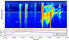 |
Fig. 1. Dynamic spectrum of the type II burst on 2011 February 14. The combined spectrum was obtained from records of the URAN-2 (10–33 MHz) and NDA (33–70 MHz) antenna arrays. The type II burst and several groups of type III bursts are denoted in the spectrogram as Type II and Type III, respectively. The lower panel shows the solar X-ray emission measured by GOES 15 on that day. The C9.4 class flare start, end, and peak times are shown as dashed vertical orange and cyan lines, respectively. The common time axis is in the range 12:40–13:15 UT. |
Figure 2 presents the URAN-2 dynamic spectrum, which shows an abundance of the fine structure within the Type II. Notably, the Type II exhibits band-splitting. It is clearly visible after ∼13:07 UT in the NDA spectrogram (see Fig. 3a). Fig. 2 only shows the LFB of the Type II. The LFB undergoes a branching into a lower lane (LL) and an upper lane (UL) in frequencies. This new peculiarity is the spectral cleaving. The dashed purple lines in the figure encompass the LFB before and after a cleaving point (CP) at 13:09:40.5 UT. Surprisingly, the UL after the CP first rises and then descends in frequency. This feature is known as a spectral bump (Koval et al. 2021). In addition, another type II burst escorts the Type II. It has both a herringbone structure and the band-splitting. This burst is labeled “HB Type II (LFB)” and “HB Type II (UFB)” in Fig. 2.
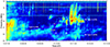 |
Fig. 2. URAN-2 dynamic spectrum with the low-frequency band of the type II burst, Type II (LFB), showing the spectral cleaving. The dashed purple lines encompass the LFB before and after the cleaving point (CP), which was at the time instant of 13:09:40.5 UT and at a frequency of 28.12 MHz. The LFB divided into a lower lane (LL) and an upper lane (UL) as a result of the spectral cleaving. The UL ascends and descends in frequency, making a spectral bump feature. The type II burst with herringbones has a band-splitting with lower and upper frequency bands, which are indicated as HB Type II (LFB) and HB Type II (UFB). |
Figure 3a demonstrates the LFB and UFB of the Type II. The HB Type II is also visible (dashed black ellipses). Visually, we fit the Type II (LFB) until the CP by linear curve (dashed blue line in the figure). This shows that the FDR of the LFB, dfLFB/dt, is equal to about −8.7 kHz/s, which is lower than typical FDRs for meter-decameter type II bursts (Aguilar-Rodriguez et al. 2005). The Type II (UFB) has a ragged appearance, but it was roughly depicted (as indicated by the dark green line in the figure). The UFB follows the UL of the Type II (LFB) by making the spectral bump. At the same time, there is no manifestation of the spectral cleaving in the UFB.
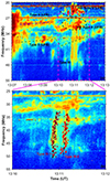 |
Fig. 3. NDA dynamic spectra with type II and type III bursts on 2011 February 14. (a) NDA dynamic spectrum with the lower and upper frequency bands of the type II burst (Type II (LFB) and Type II (UFB)) as well as the type II burst with herringbones (HB Type II (LFB) and HB Type II (UFB)). Type II (LFB) and Type II (UFB) are indicated by dashed blue and dark green lines. HB Type II (LFB) and HB Type II (UFB) are delineated by dashed black ellipses. Two type III bursts are marked as Type III. (b) NDA dynamic spectrum with the first and second type III bursts, which are labeled Type III-1 and Type III-2. The intensity maxima in each frequency channel along the bursts are shown by brown and red dots for Type III-1 and Type III-2, respectively. The dashed black lines are approximations by linear curves indicating frequency drifts. |
We noticed at least two intense type III bursts, marked as “Type III” in Fig. 3a. They are labeled “Type III-1” and “Type III-2” in Fig. 3b, which provides an enlarged view. The two bursts appear to terminate at the UL of the Type II (LFB), which is imposed on the Type II (UFB). To estimate their FDRs, we partially exploited the approach developed in Koval et al. (2023). Sequentially, the bursts were manually isolated to determine the intensity maxima in each frequency channel. Although the fitting procedure for time-frequency traces of type III burst maxima is more sophisticated (Stanislavsky et al. 2018), we fit the maxima with linear curves as a first approximation. Thus, the FDRs, dfIII/dt, are equal to −3.4 MHz/s and −2.9 MHz/s for Type III-1 and Type III-2. If they were reverse-drifting HBs of the HB Type II (UFB), they would have positive and slightly lower FDRs (Dorovskyy et al. 2015). This confirms that they belong to the type III class of solar bursts and cannot be mistaken for herringbones.
4. Interpretation
We provide an initial interpretation of the occurrence of the newly identified feature as the spectral cleaving in type II bursts. We assumed that the electrons that generate the Type II emission are accelerated by the shock-drift acceleration mechanism (Holman & Pesses 1983; Leroy & Mangeney 1984; Wu 1984; Krauss-Varban & Wu 1989; Vandas 1989; Vandas & Karlický 2011). In accordance with Ball & Melrose (2001), we considered the shock normal frame, where the plasma in the upstream region moves at a velocity u1 along the normal to the shock front. The angle between the magnetic field vector and this normal is ψ1 (Fig. 1 in Ball & Melrose 2001). Shock waves can be categorized according to the speed of the point of intersection between a particular magnetic field line and the shock front. When this speed is lower than speed of light, then a shock is subluminal. In the opposite case, it is superluminal. In the subluminal case, electrons are accelerated, and the acceleration efficiency is ∝tanψ1. Therefore, the maximum electron acceleration is at very high angles (≈90o) and depends on the shock wave parameters. On the other hand, in the superluminal case, which is valid for angles ψ1 ≃ 90o, the electron acceleration efficiency is very low (all electrons are transmitted downstream and their energy gain is very low).
Thus, sources of a type II burst emission are assumed to be located close to the regions on a shock front in which electrons are most efficiently accelerated. This implies that these regions are not everywhere at the shock front, but only where ψ1 ≈ 90o, excluding ψ1 ≃ 90o. We use this assertion and the foregoing facts to interpretate the observations described above.
Figure 3a clearly shows the band-splitting of the Type II from ∼13:07:30 UT till ∼13:09:40 UT. We assumed that two radio sources correspond to the LFB and UFB of the Type II. Moreover, the LFB radio source was assumed to be a double source composed of two components (see Fig. 4a). In general, this scenario agrees with that of Holman & Pesses (1983). Then, at about 13:09:40 UT, the Type II (LFB) divides into two lanes (LL and UL), which is the spectral cleaving (Fig. 2). We attribute the spectral cleaving to changes in the magnetic field orientation ahead of the propagating shock front. When this orientation varies, the region of the most effective electron acceleration (sources of the Type II (LFB) emission) shifts along the shock front or even diverges, as shown in the scenario in Fig. 4.
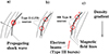 |
Fig. 4. Sketch demonstrating the possible scenario of the occurrence of the spectral cleaving in the Type II (LFB) step by step: (a) Phase before the cleaving (∼13:09:30 UT). (b) Phase after the cleaving (∼13:10:00 UT). (c) Phase after the cleaving with herringbones (∼13:11:00 UT). The short red arrows indicate the electron beams that generate herringbones. |
In our case, the shock front most likely propagates in a direction that is highly different from the radial direction in the gravitationally stratified solar atmosphere. This inference is based on the low value of the FDR of the Type II (LFB) (Fig. 2). Thus, in the Type II (LFB) during the time period of 13:07:30–13:09:40 UT, the condition (ψ1 near 90o) for the most effective acceleration is fulfilled only in the regions close to the top of the shock front (Fig. 4a), where the double source is situated (red circles in Fig. 4a). There electrons are accelerated. These suprathermal electrons gave rise to the subsequent radio emission via the plasma emission mechanism. Since the double source is rather compact, the Type II (LFB) is seen to be not cleaved in the dynamic spectrum.
Later, after 13:09:40 UT, the magnetic field lines ahead of the shock front gradually changed in such a way that around the top of the shock front, ψ1 ≃ 90o (see Fig. 4b). Consequently, due to a decrease in electron acceleration efficiency, the radio emission from this location disappeared. Simultaneously, two well-separated regions with high ψ1 (i.e., with the maximum electron acceleration) appeared along the shock front. The first radio source was located at a higher altitude in the solar atmosphere and the second source was at a lower altitude. Before 13:09:40 UT, they were the components of the double source. Due to the difference in plasma densities between higher and lower sources, the LL and UL of the Type II (LFB) were generated. This scenario agrees with that presented in Fig. 2b by Holman & Pesses (1983).
According to the URAN-2 spectrogram, the frequency bandwidth of the Type II (LFB) before its cleaving is broader than those of the UL and LL after the cleaving. Moreover, the Type II (LFB) consists of two sublanes (see Fig. 2 at 13:08:25–13:09:00 UT). This agrees with the presented scenario, where the bandwidth of the Type II (LFB) before its partition is produced by two radio sources that are close (but not at the same position), in contrast to solitary radio sources of the LL and UL after the cleaving point.
Then, two radio sources remain at about 13:10:00 UT. However, the radio source (region of acceleration) of the UL moves upward in the solar atmosphere and thus makes a bump in frequency that is known as the spectral bump. This effect can be also caused by a change in the magnetic lines orientation relative to the shock front. The spectral bump feature was also explained by interaction of a type II burst and denser coronal structure (either streamer or flux tube) in Koval et al. (2021).
During the phases before and after the spectral cleaving in the Type II (Figs. 4a,b), the radio sources are probably close to the acceleration regions. Shortly after the cleaving, at around 13:11:00 UT, the HB Type II was observed. This indicates changes in the acceleration processes at the shock front. The HB Type II is associated with two type III bursts. Moreover, its LFB and UFB occur at frequencies close to the LL and UL of the Type II. According to the models developed by Holman & Pesses (1983) and Vandas & Karlický (2011), HBs are generated by the electron beams that escape from the acceleration region that is located at a shock front. However, there is a difference between these models. Holman & Pesses only considered the electrons accelerated upstream from two regions at the shock moving nearly parallel to the solar surface (Fig. 2d in Holman & Pesses 1983). Conversely, Vandas & Karlický showed that the shock can have one acceleration region from which the electron beams propagate in the both upstream and downstream directions and thus generate HBs. Since the LFB and UFB of the HB Type II contain both forward- and reverse-drifting HBs, the concept proposed by Vandas & Karlický (2011) is more closely aligned with observations (see Fig. 4c).
In our case, the electrons that cause the HBs are expected to be accelerated at the shock front. Meanwhile, the electron beams generating the type III bursts were accelerated at some lower atmospheric heights. Therefore, the question arises whether the Type III electron beams can enhance the acceleration process at the LL and UL sources of the Type II. This could explain the appearance of HB Type II (LFB) and HB Type II (UFB) and the coincidence in time between the Type III bursts and HB Type II. If the relation between the Type III bursts and HB Type II is not accidental, then the Type III electron beams need to penetrate the region in which the electrons that produce the HBs are accelerated (see the red arrow in Fig. 4c). However, the type III burst electrons are too fast to generate the HBs directly. On the other hand, it is known that each electron beam produces a return current (see e.g. Karlický & Henoux 1992). This neutralizes the current of the electron beam. The return current heats the plasma, which can enter into the shock. In the shock, the electrons of the heated plasma are subsequently accelerated to energies that are higher than those in the case without the return current, and thus, they produce HBs. However, this conjecture needs further verification by numerical simulations and future observations.
5. Conclusions
We have reported radio observations of a previously unrecognized feature, called spectral cleaving, in solar type II bursts. We treated high-fidelity dynamic spectra obtained with the URAN-2 radio telescope on 2011 February 14. We found that the spectral cleaving is a new distinct spectral effect indicative of involuted plasma processes that occur within the solar corona. We proved that the spectral cleaving differs from the well-known band-splitting not only in its morphology, but also in the underlying physical mechanism, highlighting the complexity of this phenomenon. These discoveries not only enrich our knowledge of the solar radio emission, but also provide valuable insights into fundamental plasma physics processes taking place in astrophysical environments.
We offered an initial interpretation of the spectral cleaving in type II bursts. The intricate interplay between the shock wave and magnetic field configurations plays a key role here. The efficient acceleration of electrons, which leads to subsequent type II radio emission, is typically associated with a quasi-perpendicular shock-to-magnetic-field orientation (Kong et al. 2015). However, it is unlikely that this orientation remains constant throughout the shock wave propagation in the solar corona. It seems more plausible that the orientation varies on spatial and temporal scales ∼1 R⊙ (Knock & Cairns 2005; Cho et al. 2013) and up to 30 minutes (Alissandrakis & Gary 2021) for the metric type II radio bursts. We recall that the duration of the type II burst we studied was about 13 minutes, while the shock wave traveled a distance of about 0.5 R⊙ (Fig. 4b in Yashiro et al. 2014). We assume that the shift (or migration) of the radio sources along the shock front takes place due to the occurrence of spectral cleaving, precisely because of the change in orientation. It should be noted that more than one radio source can appear at the beginning of type II radio emission. If they are spatially close to each other, they are unresolved in a spectrogram, and only one type II lane is present. This was the case here.
The proposed interpretation of the spectral cleaving phenomenon is new and may hold for solar type II radio bursts in a wider context. Generally, most type II bursts display intermittent shapes as they drift in spectrograms. We suggest that this reflects the change in the above-described orientation and hence the migration of radio source(s). In this case, the level of this intermittency depends on the similar geometry of a shock front and magnetic field topology in the solar corona. Therefore, moderate migrations of a radio source may result in modest pulsations in a type II burst lane. However, stronger migrations reveal themselves, for example, through spectral cleaving features. Only a simultaneous examination of radio spectral and imaging observations of spectral cleaving in type II bursts will reveal more about this phenomenon. For this task, we consider the radio facilities URAN-2, UTR-2, GURT (Konovalenko et al. 2016), LOFAR and the New Extension in Nançay Upgrading LOFAR (NenuFAR; Zarka et al. (2020)) to be best suited. An analysis of the data from these radio telescopes, which provide records with high frequency and temporal resolutions in wide dynamic ranges, would be highly valuable.
Acknowledgments
A.K., M.K., M.V., M.B. were supported by the project RVO:67985815. A.K., M.K., M.B. acknowledge support from Grant 22-34841S of the Czech Science Foundation. We thank the radio monitoring service at LESIA (Observatoire de Paris) for providing value-added data that have been used for this study. We are grateful to all those who contributed to the operation of GOES, STEREO, and RSTN instruments.
References
- Aguilar-Rodriguez, E., Gopalswamy, N., MacDowall, R., et al. 2005, in Proc. Solar Wind 11/SOHO 16, Connecting Sun and Heliosphere (ESA SP-592), eds. B. Fleck, T. H. Zurbuchen, & H. Lacoste (Noordwijk: ESA), 147, 393 [Google Scholar]
- Alissandrakis, C. E., & Gary, D. E. 2021, Front. Astron. Space Sci., 7, 77 [CrossRef] [Google Scholar]
- Ball, L., & Melrose, D. B. 2001, PASA, 18, 361 [NASA ADS] [CrossRef] [Google Scholar]
- Bhunia, S., Carley, E. P., Oberoi, D., & Gallagher, P. T. 2023, A&A, 670, A169 [NASA ADS] [CrossRef] [EDP Sciences] [Google Scholar]
- Cairns, I. H., & Robinson, R. D. 1987, Sol. Phys., 111, 365 [Google Scholar]
- Carley, E. P., Reid, H. A., Vilmer, N., & Gallagher, P. T. 2015, A&A, 581, A100 [NASA ADS] [CrossRef] [EDP Sciences] [Google Scholar]
- Cho, K.-S., Gopalswamy, N., Kwon, R.-Y., et al. 2013, ApJ, 765, 148 [NASA ADS] [CrossRef] [Google Scholar]
- Chrysaphi, N., Kontar, E. P., Holman, G. D., & Temmer, M. 2018, ApJ, 868, 79 [NASA ADS] [CrossRef] [Google Scholar]
- Dorovskyy, V. V., Melnik, V. N., Konovalenko, A. A., et al. 2015, Sol. Phys., 290, 2031 [NASA ADS] [CrossRef] [Google Scholar]
- Gopalswamy, N., Yashiro, S., Kaiser, M. L., et al. 2001, ApJ, 548, 1 [NASA ADS] [CrossRef] [Google Scholar]
- Gopalswamy, N., Yashiro, S., Kaiser, M. L., et al. 2002, Geophys. Res. Lett., 29, 8 [CrossRef] [Google Scholar]
- Holman, G. D., & Pesses, M. E. 1983, ApJ, 267, 837 [NASA ADS] [CrossRef] [Google Scholar]
- Howard, R. A., Moses, J. D., Vourlidas, A., et al. 2008, Space Sci. Rev., 136, 67 [NASA ADS] [CrossRef] [Google Scholar]
- Kaiser, M. L., Kucera, T. A., Davila, J. M., et al. 2008, Space Sci. Rev., 135, 5 [NASA ADS] [CrossRef] [Google Scholar]
- Karlický, M., & Henoux, J.-C. 1992, A&A, 264, 679 [NASA ADS] [Google Scholar]
- Knock, S. A., & Cairns, I. H. 2005, J. Geophys. Res.: Space Phys., 110, A1 [CrossRef] [Google Scholar]
- Kong, X. L., Chen, Y., Guo, F., et al. 2015, ApJ, 798, 81 [Google Scholar]
- Konovalenko, A., Sodin, L., Zakharenko, V., et al. 2016, Exp. Astron., 42, 1 [Google Scholar]
- Koval, A., Karlický, M., Stanislavsky, A., et al. 2021, ApJ, 923, 255 [NASA ADS] [CrossRef] [Google Scholar]
- Koval, A., Stanislavsky, A., Karlický, M., et al. 2023, ApJ, 952, 51 [NASA ADS] [CrossRef] [Google Scholar]
- Krauss-Varban, D., & Wu, C. S. 1989, J. Geophys. Res., 94, A11 [NASA ADS] [Google Scholar]
- Lecacheux, A. 2000, Geophys. Monogr. Ser., 119, 321 [NASA ADS] [Google Scholar]
- Leroy, M. M., & Mangeney, A. 1984, Ann. Geophys., 2, 449 [NASA ADS] [Google Scholar]
- Magdalenić, J., Marqué, C., Fallows, R. A., et al. 2020, ApJ, 897, L15 [Google Scholar]
- Mäkelä, P., Gopalswamy, N., & Akiyama, S. 2018, ApJ, 867, 40 [Google Scholar]
- Mancuso, S., & Raymond, J. C. 2004, A&A, 202, 363 [NASA ADS] [CrossRef] [EDP Sciences] [Google Scholar]
- Mann, G., Vocks, C., Warmuth, A., et al. 2022, A&A, 660, A71 [NASA ADS] [CrossRef] [EDP Sciences] [Google Scholar]
- McLean, D. J. 1967, PASA, 1, 47 [Google Scholar]
- McLean, D. J., & Labrum, N. R. 1985, Solar Radiophysics: Studies of Emission from the Sun at Metre Wavelengths (Cambridge: Cambridge Univ. Press) [Google Scholar]
- Mel’nik, V. N., Konovalenko, A. A., Rucker, H. O., et al. 2004, Sol. Phys., 222, 1 [CrossRef] [Google Scholar]
- Reid, H. A. S., & Ratcliffe, H. 2014, Res. Astron. Astrophys., 14, 773 [Google Scholar]
- Reid, H. A. S., & Kontar, E. P. 2017, A&A, 606, A141 [NASA ADS] [CrossRef] [EDP Sciences] [Google Scholar]
- Roberts, J. A. 1959, Aust. J. Phys., 12, 327 [Google Scholar]
- Smerd, S. F., Sheridan, K. V., & Stewart, R. T. 1975, Astrophys. Lett., 16, 23 [NASA ADS] [Google Scholar]
- Stanislavsky, A. A., Konovalenko, A. A., Koval, A. A., et al. 2015, Sol. Phys., 290, 1 [Google Scholar]
- Stanislavsky, L. A., Bubnov, I. N., Konovalenko, A. A., et al. 2017, Res. Astron. Astrophys., 21, 187 [Google Scholar]
- Stanislavsky, A. A., Konovalenko, A. A., Abranin, E. P., et al. 2018, Sol. Phys., 293, 11 [NASA ADS] [CrossRef] [Google Scholar]
- Stanislavsky, A. A., Bubnov, I. N., Koval, A. A., & Yerin, S. N. 2022, A&A, 657, A21 [NASA ADS] [CrossRef] [EDP Sciences] [Google Scholar]
- Tingay, S. J., Goeke, R., Bowman, J. D., et al. 2013, PASA, 30 [CrossRef] [Google Scholar]
- van Haarlem, M. P., Wise, M. W., Gunst, A. W., et al. 2013, A&A, 556, A2 [NASA ADS] [CrossRef] [EDP Sciences] [Google Scholar]
- Vandas, M. 1989, Bull. Astron. Inst. Czechosl., 40, 175 [NASA ADS] [Google Scholar]
- Vandas, M., & Karlický, M. 2011, A&A, 531, A55 [NASA ADS] [CrossRef] [EDP Sciences] [Google Scholar]
- Vršnak, B., Magdalenić, J., Aurass, H., & Mann, G. 2002, A&A, 396, 673 [NASA ADS] [CrossRef] [EDP Sciences] [Google Scholar]
- Wu, C. S. 1984, J. Geophys. Res., 89, A10 [Google Scholar]
- Yashiro, S., Mäkelä, P., Gopalswamy, N., et al. 2014, Adv. Space Res., 54, 8 [Google Scholar]
- Zarka, P., Denis, L., Tagger, M., et al. 2020, URSI GASS 2020, Session J01 New Telescopes on the Frontier, https://tinyurl.com/ycocd5ly [Google Scholar]
- Zhang, J., & Wang, J. 2002, ApJ, 566, 2 [NASA ADS] [Google Scholar]
- Zhang, P., Morosan, D., Zucca, P., et al. 2024a, A&A, 684, L22 [NASA ADS] [CrossRef] [EDP Sciences] [Google Scholar]
- Zhang, P., Morosan, D., Kumari, A., & Kilpua, E. 2024b, A&A, 683, A123 [NASA ADS] [CrossRef] [EDP Sciences] [Google Scholar]
- Zimovets, I. V., & Sadykov, V. M. 2015, Adv. Space Res., 56, 2811 [NASA ADS] [CrossRef] [Google Scholar]
All Figures
|
Fig. 1. Dynamic spectrum of the type II burst on 2011 February 14. The combined spectrum was obtained from records of the URAN-2 (10–33 MHz) and NDA (33–70 MHz) antenna arrays. The type II burst and several groups of type III bursts are denoted in the spectrogram as Type II and Type III, respectively. The lower panel shows the solar X-ray emission measured by GOES 15 on that day. The C9.4 class flare start, end, and peak times are shown as dashed vertical orange and cyan lines, respectively. The common time axis is in the range 12:40–13:15 UT. |
| In the text | |
|
Fig. 2. URAN-2 dynamic spectrum with the low-frequency band of the type II burst, Type II (LFB), showing the spectral cleaving. The dashed purple lines encompass the LFB before and after the cleaving point (CP), which was at the time instant of 13:09:40.5 UT and at a frequency of 28.12 MHz. The LFB divided into a lower lane (LL) and an upper lane (UL) as a result of the spectral cleaving. The UL ascends and descends in frequency, making a spectral bump feature. The type II burst with herringbones has a band-splitting with lower and upper frequency bands, which are indicated as HB Type II (LFB) and HB Type II (UFB). |
| In the text | |
|
Fig. 3. NDA dynamic spectra with type II and type III bursts on 2011 February 14. (a) NDA dynamic spectrum with the lower and upper frequency bands of the type II burst (Type II (LFB) and Type II (UFB)) as well as the type II burst with herringbones (HB Type II (LFB) and HB Type II (UFB)). Type II (LFB) and Type II (UFB) are indicated by dashed blue and dark green lines. HB Type II (LFB) and HB Type II (UFB) are delineated by dashed black ellipses. Two type III bursts are marked as Type III. (b) NDA dynamic spectrum with the first and second type III bursts, which are labeled Type III-1 and Type III-2. The intensity maxima in each frequency channel along the bursts are shown by brown and red dots for Type III-1 and Type III-2, respectively. The dashed black lines are approximations by linear curves indicating frequency drifts. |
| In the text | |
|
Fig. 4. Sketch demonstrating the possible scenario of the occurrence of the spectral cleaving in the Type II (LFB) step by step: (a) Phase before the cleaving (∼13:09:30 UT). (b) Phase after the cleaving (∼13:10:00 UT). (c) Phase after the cleaving with herringbones (∼13:11:00 UT). The short red arrows indicate the electron beams that generate herringbones. |
| In the text | |
Current usage metrics show cumulative count of Article Views (full-text article views including HTML views, PDF and ePub downloads, according to the available data) and Abstracts Views on Vision4Press platform.
Data correspond to usage on the plateform after 2015. The current usage metrics is available 48-96 hours after online publication and is updated daily on week days.
Initial download of the metrics may take a while.