| Issue |
A&A
Volume 689, September 2024
|
|
|---|---|---|
| Article Number | A43 | |
| Number of page(s) | 12 | |
| Section | Extragalactic astronomy | |
| DOI | https://doi.org/10.1051/0004-6361/202450153 | |
| Published online | 30 August 2024 | |
Very-long-baseline interferometry study of the flaring blazar TXS 1508+572 in the early Universe
1
Max-Planck-Institut für Radioastronomie, Auf dem Hügel 69, 53121 Bonn, Germany
e-mail: This email address is being protected from spambots. You need JavaScript enabled to view it.
2
Julius-Maximilians-Universität Würzburg, Fakultät für Physik und Astronomie, Institut für Theoretische Physik und Astrophysik, Lehrstuhl für Astronomie, Emil-Fischer-Str. 31, 97074 Würzburg, Germany
3
Department of Physics & McDonnell Center for the Space Sciences, Washington University in St. Louis, One Brookings Drive, St. Louis, MO 63130, USA
4
Instituto de Física, Pontificia Universidad Católica de Valparaíso, Casilla 4059, Valparaíso, Chile
5
Astro Space Center of Lebedev Physical Institute, Profsouznaya 84/32, Moscow 117997, Russia
6
Joint Institute for VLBI ERIC, Oude Hoogeveensedijk 4, 7991 PD Dwingeloo, The Netherlands
7
Faculty of Aerospace Engineering, Delft University of Technology, Kluyverweg 1, 2629 HS Delft, The Netherlands
Received:
27
March
2024
Accepted:
1
June
2024
Abstract
Context. High-redshift blazars provide valuable input to studies of the evolution of active galactic nuclei (AGN) jets and provide constraints on cosmological models. Detections at high energies (0.1 < E < 100 GeV) of these distant sources are rare, but when they exhibit bright gamma-ray flares, we are able to study them. However, contemporaneous multi-wavelength observations of high-redshift objects (z > 4) during their different periods of activity have not been carried out so far. An excellent opportunity for such a study arose when the blazar TXS 1508+572 (z = 4.31) exhibited a γ-ray flare in 2022 February in the 0.1 − 300 GeV range with a flux 25 times brighter than the one reported in the in the fourth catalog of the Fermi Large Area Telescope.
Aims. Our goal is to monitor the morphological changes, spectral index and opacity variations that could be associated with the preceding γ-ray flare in TXS 1508+572 to find the origin of the high-energy emission in this source. We also plan to compare the source characteristics in the radio band to the blazars in the local Universe (z < 0.1). In addition, we aim to collect quasi-simultaneous data to our multi-wavelength observations of the object, making TXS 1508+572 the first blazar in the early Universe (z > 4) with contemporaneous multi-frequency data available in its high state.
Methods. In order to study the parsec-scale structure of the source, we performed three epochs of very-long-baseline interferometry (VLBI) follow-up observations with the Very Long Baseline Array (VLBA) supplemented with the Effelsberg 100-m Telescope at 15, 22, and 43 GHz, which corresponds to 80, 117, and 228 GHz in the rest frame of TXS 1508+572. In addition, one 86 GHz (456 GHz) measurement was performed by the VLBA and the Green Bank Telescope during the first epoch.
Results. We present total intensity images from our multi-wavelength VLBI monitoring that reveal significant morphological changes in the parsec-scale structure of TXS 1508+572. The jet proper motion values range from 0.12 mas yr−1 to 0.27 mas yr−1, which corresponds to apparent superluminal motion βapp ≈ 14.3 − 32.2 c. This is consistent with the high Lorentz factors inferred from the spectral energy distribution (SED) modeling for this source. The core shift measurement reveals no significant impact by the high-energy flare on the distance of the 43-GHz radio core with respect to the central engine, that means this region is probably not affected by e.g., injection of new plasma as seen in other well-studied sources like CTA 102. We determine the average distance from the 43-GHz radio core to the central supermassive black hole to be 46.1 ± 2.3 μas, that corresponds to a projected distance of 0.32 ± 0.02 pc. We estimate the equipartition magnetic field strength 1 pc from the central engine to be on the order of 1.8 G, and the non-equipartition magnetic field strength at the same distance to be about 257 G, the former of which values agrees well with the magnetic field strength measured in low to intermediate redshift AGN.
Conclusions. Based on our VLBI analysis, we propose that the γ-ray activity observed in February 2022 is caused by a shock-shock interaction between the jet of TXS 1508+572 and new plasma flowing through this component. Similar phenomena have been observed, for example, in CTA 102 in a shock-shock interaction between a stationary and newly emerging component. In this case, however, the core region was also affected by the flare as the core shift stays consistent throughout the observations.
Key words: techniques: high angular resolution / techniques: interferometric / galaxies: active / galaxies: jets / radio continuum: galaxies
© The Authors 2024
 Open Access article, published by EDP Sciences, under the terms of the Creative Commons Attribution License (https://creativecommons.org/licenses/by/4.0), which permits unrestricted use, distribution, and reproduction in any medium, provided the original work is properly cited.
This article is published in open access under the Subscribe to Open model.
Open access funding provided by Max Planck Society.
1. Introduction
Blazars, a subclass of radio-loud active galactic nuclei (AGN) whose jets point toward the observer (Urry & Padovani 1995), are among the most luminous objects in the Universe. They emit radiation throughout the whole electromagnetic spectrum, and their spectral energy distribution (SED) shows a double-humped structure (Padovani & Giommi 1995). In leptonic models, the low-energy hump, stretching from the radio to the ultraviolet, and sometimes even to the X-ray band, arises from synchrotron and the high-energy hump (X-rays to γ-rays) originates from inverse Compton scattering (IC). Depending on the origin of the seed photon field, the IC process can be either synchrotron self-Compton (SSC) or external Compton (EC) with seed photons from the broad-line region and/or the dusty torus. Alternatively, hadronic models (e.g., proton synchrotron) can also be responsible for the high-energy emission (e.g., Aharonian 2002; Böttcher et al. 2013). High-redshift blazars that existed when the Universe was only ∼1 Gyr old already harbored supermassive black holes (SMBHs, MBH ≥ 109 M⊙) in their central engines (Bloemen et al. 1995; Ghisellini et al. 2010). However, it is not yet clear how these objects could have formed so early in the Universe, but studies by Jolley & Kuncic (2008) and Ghisellini et al. (2013) suggest that AGN feedback can boost accretion onto the central engine and accelerate black hole growth. Thus, investigating the properties of high-redshift blazars can help us to better understand SMBH and AGN evolution, as well as the intricacies of AGN feedback on their host galaxies (Volonteri 2010).
Blazars are the most abundant sources on the extragalactic γ-ray sky. While over half of the 5064 sources contained in the fourth catalog of the Fermi Large Area Telescope (LAT, Atwood et al. 2009) are blazars, only 33 of these sources are categorized as high redshift objects (z > 2.5 cutoff set by the LAT, Abdollahi et al. 2020). However, most of these high-redshift sources can only be detected by the LAT during flaring states (Paliya et al. 2019; Kreter et al. 2020), otherwise their steeply falling spectra prevent their detection at low states in the GeV energy range. This complicates obtaining quasi-simultaneous multi-wavelength observational data for studies of their broadband emission. The only example of such a quasi-simultaneous study to date is the case of the intermediate-redshift object TXS 0536+145 at z = 2.69 (Orienti et al. 2014).
TXS 1508+572 (also called GB6 B1508+5714, J1510+5702) is a high-redshift blazar at z = 4.31 (Hook et al. 1995; Schneider et al. 2007). On kiloparsec scales, the source shows a double-sided jet structure (Kappes et al. 2022) in the east-west direction. The first very-long-baseline interferometry (VLBI) image of TXS 1508+572 was published by Frey et al. (1997), and the resulting 5 GHz map shows an unresolved source structure with the synthesized beam of ∼5 mas. However, global VLBI observations at 5 and 8.4 GHz revealed an optically thin jet component at 5 GHz and 8.4 GHz about 2 mas south of the core (O’Sullivan et al. 2011). The AstroGeo Database1 provides 8.7 GHz images of the source with a compact core-jet morphology and the jet oriented toward southwest. Kinematic analysis based on 4 years of 8.6 GHz observations reveals a jet proper motion of 0.117 ± 0.078 mas yr−1 (Titov et al. 2023).
A strong γ-ray flare was detected in TXS 1508+572 on 2022 February 4 (Gokus et al. 2022) with a γ-ray monitoring program following the high-z blazar detection method described in Kreter et al. (2020). We have started a multi-frequency campaign across the electromagnetic spectrum to follow up this event with quasi-simultaneous observations (see Paper I, Gokus et al. 2024). Since γ-ray observations lack the resolution required for determining the origin of the activity, we have initiated a multi-frequency VLBI monitoring to capture the evolution of the source morphology and, possibly, relate VLBI structural components to the observed high-energy activity. To the best of our knowledge, such an immediate follow-up observing campaign has never been carried before for any blazar at such a high redshift.
In Sect. 2 we describe VLBI observations aimed to trace the source’s morphological evolution during its high state. Section 3 describes the analysis of the observing data. Our results are discussed in Sect. 4, and we summarize our findings in Sect. 5. In this work we assume a ΛCDM cosmology with H0 = 70.7 km s−1 Mpc−1, ΩΛ = 0.73, and ΩM = 0.27 (Salvatelli et al. 2013). At the redshift of z = 4.31, this corresponds to a scale of 6.9 pc mas−1, and a luminosity distance of DL ≈ 40 Gpc.
2. Observations and data reduction
To correlate the γ-ray activity with possible parsec-scale morphological changes in TXS 1508+572, we requested three Very Long Baseline Array (VLBA) and Effelsberg observations at 15, 22, and 43 GHz, as well as an additional observation with the VLBA and the Green Bank Telescope (GBT) at 86 GHz (PIs: A. Gokus, M. Lisakov, project code: BG281).
Observations are summarized in Table 1. The correlation was carried out using the VLBA DiFX correlator (Deller et al. 2007, 2011), in 4 subbands (intermediate frequencies or IFs) and two circular polarizations, each with 256 spectral channels and a bandwidth of 128 MHz. The integration time was 0.5 s for the 86 GHz observations and 1 s for all other observations. The source 1803+784 was used as a fringe finder calibrator in all experiments.
Summary of our VLBI observations.
We performed the calibration according to the standard recipes in the Astronomical Image Processing Software (AIPS, Greisen 2003). After loading the data to AIPS using FITLD, we applied parallactic angle and digital sampling corrections. Amplitude calibration was performed based on the system noise temperature and elevation dependent gain curves provided by the stations. Opacity corrections were also applied at this step based on the weather information recorded at each antenna site. We used FRING to determine phase delay and rate solutions, and applied them both to the calibrator and target using CLCAL. It is worthwhile to highlight the importance of the GBT in the 86-GHz observation, because sufficiently high signal-to-noise ratio (S/N) fringe detections (S/N > 5) were only found on GBT baselines. These solutions were applied to the data and the fringe fit was repeated setting delay and rate windows of 200 ns and 200 mHz, and lowering the S/N cutoff to 3.7.
We corrected the flux density scale based on the quasi-simultaneous single-dish observations at 20, 14, and 7 mm of TXS 1508+572 with the Effelsberg 100-m telescope2 (see Fig. 1). Observations and data reduction was carried out as described in Eppel et al. (2024). The data was then averaged in frequency with SPLIT and written out for imaging.
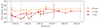 |
Fig. 1. Radio light curve of TXS 1508+572 observed with the Effelsberg 100-m telescope after the γ-ray flare (dashed black line). The VLBI observations are marked with black dotted lines. |
Hybrid imaging was performed in Difmap (Shepherd 1997) with iterating clean and phase and amplitude self-calibration with decreasing solution interval ranging from 180 to 1 min. Due to the low quality of the 86-GHz data (see Fig. 2), the imaging was carried out in two ways: assuming the same source structure as seen at lower frequencies, that is loading the 43-GHz clean windows to image the 86-GHz data; and assuming a core-dominated source. The latter yields a better map, because we do not detect any significant emission at the location of the 43-GHz jet component. Resulting maps are displayed in Figs. 3 and 4 and their properties are tabulated in Table A.1.
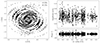 |
Fig. 2. Left panel: (u, v) coverage of the 43-GHz VLBA and EF (grey) and the 86-GHz VLBA and GBT (black) observations, plotting the fringe detections. Right panel: self-calibrated amplitude and phase of the 86-GHz data set. |
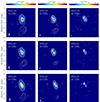 |
Fig. 3. Clean images of TXS 1508+572 at 15, 22, and 43 GHz. The observations were carried out in 2022 March, September, and in 2023 January (see Table 1). Image properties are summarized in Table A.1. Contours and colors represent the brightness distribution of the parsec-scale structure of the object. The images are aligned based on the core shift measurement. |
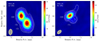 |
Fig. 4. 43 and 86 GHz image of TXS 1508+572 observed with the VLBA+EF (43 GHz, left) and VLBA+GBT (86 GHz, right). Lowest contours are at 0.53 and 1.37 mJy beam−1, and increase as a factor of two. Positions of the modelfit components are overlaid as black circles. |
3. Data analysis
3.1. Model fitting of individual source components
To be able to track individual components, as well as their brightness and kinematic evolution, we modeled the source structure with delta and elliptical Gaussian components using the modelfit command in Difmap (see Table A.2). The source is usually well modeled with four components representing the core, two jet components, and the lobe. To measure the jet components’ proper motion, μ, we calculated the angular separation between the core and jet components and fitted the obtained values using linear regression. Results from our kinematic measurements are shown in Fig. 5. The obtained values of proper motion are μ15, C1 = 0.19 ± 0.12 mas yr−1, μ15, C2 = 0.27 ± 0.16 mas yr−1, μ22, C1 = 0.20 ± 0.09 mas yr−1, μ22, C2 = 0.21 ± 0.10 mas yr−1, μ43, C1 = 0.12 ± 0.20, and μ43, C2 = 0.15 ± 0.29 mas yr−1 at 15, 22, and 43 GHz, respectively. These values are somewhat higher than the value μ8 = 0.117 ± 0.078 mas yr−1 from Titov et al. (2023) based on observations at 8 GHz (see Sect. 4.2). In Appendix B we discuss the multi-frequency kinematic analysis of the two jet components.
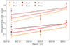 |
Fig. 5. Kinematics of the jet component at 15 (orange circles), 22 (red squares), and 43 GHz (dark red triangles) following the γ-ray flare. Jet speeds are listed in the text in Sect. 3. The positional errors are assumed to be one fifth of the beam minor axis. Note the systematic offset of the position of both jet components at the higher frequencies, which is roughly consistent with the core shift determined in Sect. 4.3. |
We calculated the brightness temperature in the source frame, Tb, obs, the following way:
![Mathematical equation: $$ \begin{aligned} T_{\mathrm{b, obs} }\,[\mathrm{K} ] = 1.22\times 10^{12} \Bigg (\frac{{S\!}_{\nu }}{\mathrm{Jy} }\Bigg ) \Bigg (\frac{\nu }{\mathrm{GHz} }\Bigg )^{-2} \Bigg (\frac{b_{\mathrm{comp} }}{\mathrm{mas} }\Bigg )^{-2} (1+z), \end{aligned} $$](/articles/aa/full_html/2024/09/aa50153-24/aa50153-24-eq1.gif) (1)
(1)
where Sν is the flux density of the components, ν is the observing frequency and bcomp is the size (full width at half maximum, FWHM) of the component. If a component is not resolved according to the resolution limit calculated based on Eq. (2) from Kovalev et al. (2005), we give an upper limit on the component size, and calculate a lower limit for Tb, obs. These values are listed in Table A.2. Taking Doppler boosting into account with a Doppler factor of δ ≈ 20, all values are below the equipartition brightness temperature of Teq ≈ 5 × 10¹⁰ K (Readhead 1994).
3.2. Spectral index maps and core shift measurements
To create spectral index maps, we re-mapped the image pairs in order for them to have a similar (u, v) range, pixel size, and restoring beam size. Images were then aligned on the optically thin jet components using 2D cross-correlation. Spectral index maps are displayed in Fig. A.2, and spectra of the core and jet components are shown in Fig. A.1. In the Blandford–Königl jet model (Blandford & Königl 1979), the VLBI core represents the τ = 1 optical depth to synchrotron radiation, whose geometry is frequency dependent. As a result of this, higher frequency observations probe the regions closer to the central engine, and one can extrapolate the location of the SMBH based on the relative frequency-dependent shifts of the optically thick core determined from pairs of images at different frequencies (Marcaide & Shapiro 1984; Lobanov 1998). For our analysis, we use the 43 GHz core as a reference. Our core shift measurement is carried out the same way as described in Pushkarev et al. (2012), aligning the images using the shifts obtained from 2D cross-correlation, and measuring the difference between the core positions of consecutive frequency pairs. The alignment error was assumed to be half of the pixel size of a given frequency pair, and the core position errors were estimated based on the χ2 minimization method described in Lampton et al. (1976). Under the assumption of equipartition, conserved magnetic flux, as well as that both the particle density and the magnetic field decrease with the distance from the central engine (Lobanov 1998), we can then measure the apparent distance between the VLBI core and the jet apex as:
![Mathematical equation: $$ \begin{aligned} \Delta r_{\mathrm{core} }\,[\upmu \mathrm{as}] = r_0 \Bigg [\Bigg (\frac{\nu }{43\,\mathrm{GHz} }\Bigg )^{-1/k_{\mathrm{r} }}-1\Bigg ], \end{aligned} $$](/articles/aa/full_html/2024/09/aa50153-24/aa50153-24-eq2.gif) (2)
(2)
where r0 is the distance between the jet apex and the 43 GHz core. kr = 1 corresponds to a conical jet width profile. The results of our core shift analysis are shown in Fig. 6.
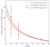 |
Fig. 6. Evolution of the core shift measured throughout the first (gold), second (red), and third (purple) VLBI epochs. The distance to the jet apex (r0) is shown in the legend for each of the three epochs. |
Based on the core shift measurement, we estimate the magnetic field strength using the methods described in Lobanov (1998), Hirotani (2005), Zdziarski et al. (2015) and Lisakov et al. (2017). First, we calculate Ωr, ν, the shift in parsec per unit 1/ν difference:
![Mathematical equation: $$ \begin{aligned} \Omega _{\mathrm{r} \nu } [\mathrm {pc\,GHz}^{\mathrm{k} _{\mathrm{r} }}] = 4.85\times 10^{-9} \frac{\Delta r_{\mathrm{core} }D_{\mathrm{L} }}{(1+z)^2} \frac{\nu _1^{1/k_{\mathrm{r} }} \nu _2^{1/k_{\mathrm{r} }}}{\nu _2^{1/k_{\mathrm{r} }}-\nu _1^{1/k_{\mathrm{r} }}}, \end{aligned} $$](/articles/aa/full_html/2024/09/aa50153-24/aa50153-24-eq3.gif) (3)
(3)
where Δrcore is the core shift between frequencies ν1 and ν2. To derive an upper limit on the magnetic field strength, we calculate the core shift and Ωrν between 15 and 43 GHz.
The magnetic field strength 1 pc from the jet apex under the equipartition assumption is calculated as (Zdziarski et al. 2015):
![Mathematical equation: $$ \begin{aligned} B^{\mathrm{eq} }_{\rm 1\,pc } [\mathrm{G}] \approx 0.025 \Bigg [\frac{\Omega ^{3k_{\mathrm{r} }}_{r\nu } (1+z)^{3}}{\delta ^{2} \phi \sin ^{3k_{\mathrm{r} }-1}\theta } \Bigg ]^{\frac{1}{4}}, \end{aligned} $$](/articles/aa/full_html/2024/09/aa50153-24/aa50153-24-eq4.gif) (4)
(4)
where ϕ is the intrinsic opening angle and θ is the viewing angle. For the viewing angle we adopted the same value as the one used for the SED fit in Paper I, θ = 1/20 rad. We calculated the apparent half opening angle based on the size of the modelfit components as ϕapp = arctan[(bjet − bcore)/d], which are the sizes of the jet, bjet, and core components, bcore, and the distance between these components, d. We did this for all observations and adopted ϕapp as the average of these values, (9 ± 2)°. The intrinsic full opening angle was calculated as ϕ = 2arctan(tanϕapp sin θ), which is (0.9 ± 0.2)°.
We also calculate the magnetic field strength 1 pc from the central SMBH, without assuming equipartition (Zdziarski et al. 2015):
![Mathematical equation: $$ \begin{aligned} B^{\mathrm{non-eq} }_{\rm 1\,pc } [\mathrm{G} ] \approx \frac{3.35\times 10^{-11}\,D_{\rm L} \Delta r_{\mathrm{core} } \delta \tan {\phi }}{(\nu _1^{-1} - \nu _2^{-1})^5 [(1+z) \sin {\theta }]^3 F_{\nu }^2}, \end{aligned} $$](/articles/aa/full_html/2024/09/aa50153-24/aa50153-24-eq5.gif) (5)
(5)
where Fν is the flux density in the flat part of the spectrum.
The equipartition magnetic field strengths,  , derived for the three considered epochs are the following: 1.91 ± 0.11 G, 1.57 ± 0.17 G, and 1.79 ± 0.16 G. The
  values for the same epochs are 324.7 ± 156.3 G, 104.9 ± 82.7 G, and 341.9 ± 225.2 G, respectively.
In order to compare Beq to that of M 87 on horizon scales (Event Horizon Telescope Collaboration 2021), we extrapolate the average Beq, aver = 0.79 ± 0.04 G to 5 rg or 0.0036 pc projected distance. The gravitational radius is calculated as rg = GMBH/c2, where G is the gravitational constant and MBH is the black hole mass assumed to be 1.5 × 10¹⁰ M⊙ based on the SED fit parameters in Gokus et al. (2024). We measure  G, that is significantly larger than the B ∼ 1 − 30 G reported for M 87 (Event Horizon Telescope Collaboration 2021).
4. Discussion
4.1. Change in source morphology related to the γ-ray flare
Our VLBI observing campaign on TXS 1508+572 started after the detection of a bright γ-ray flare on 2022 February 4. Our observations at 15, 22, and 43 GHz correspond to 80, 117, and 228 GHz in the rest frame of the source given its redshift z = 4.3. Our observation at 86 GHz (456 GHz in the rest frame of the object) carried out with the VLBA and the GBT reaches frequency ranges similar to what is currently available with the Event Horizon Telescope (Event Horizon Telescope Collaboration 2019). At these observing frequencies we expect to probe the jet components in the optically thin regime.
Hybrid images from our multi-frequency observations are shown in Fig. 3. We identify the core to be the northeastern component, as it has a flat spectrum (see Fig. A.2), and it is more compact than the southwestern jet component (Table A.2). We denote the southernmost faint, diffuse component as the lobe. Its position coincides with the jet detected at 8.6 GHz by Titov et al. (2023), and it is most likely the remnant of previous activity of the blazar. 1.7 and 4.8-GHz very high resolution RadioAstron space VLBI observations reveal a similar source structure to what we observe in our images (L. I. Gurvits, priv. comm.). The 43 and 86 GHz images of TXS 1508+572 show only a compact core-jet morphology. Comparing the structure seen at 144 MHz with LOFAR (Kappes et al. 2022) and at 1.4 GHz with the VLA (Cheung 2004) to our high-frequency images, we note a difference in the jet orientation on kiloparsec and parsec scales. This projection effect, when the intrinsic bending of the jet is amplified via beaming, is commonly seen in AGN (Pearson & Readhead 1988; Conway & Murphy 1993).
4.2. Kinematics at high redshifts
While VLBI observations can measure intrinsic characteristics and kinematic properties of AGN jets, investigating high-redshift sources is challenging due to several reasons. As a result of their Doppler-boosted emission, blazars with compact core-jet structures tend to dominate flux limited AGN samples at any given redshift. In the case of AGN oriented at large angles to our line of sight, however, the steep-spectrum jet emission is too weak to be detected at high rest frame frequencies (Gurvits 2000). In addition, due to the time dilation caused by the expansion of the Universe, component movements are visible only on longer time intervals. The first jet proper motion measurements at z > 5 were performed by Frey et al. (2015) with the cadence of 7 yr or 1.17 yr in the rest frame of the target, J1026+2542. While high-redshift AGN are being targeted by VLBI observations more frequently (Krezinger et al. 2022, and references therein), kinematic analysis is only available for a small subset of them (Frey et al. 1997; Veres et al. 2010; Frey et al. 2015; Perger et al. 2018; An et al. 2020; Zhang et al. 2020, 2022; Gabányi et al. 2023; Gurvits et al. 2023, and references therein). Expanding this sample is crucial to widen our knowledge on the evolution of black hole jets. Kinematic analysis enable us to measure the bulk Lorentz factor and Doppler boosting factors, as well as the jet viewing angle. In addition, these observational data can be used to constrain SED model parameters (see Paper I), and can also be compared with the characteristics of local AGN. While high-redshift sources show only mildly relativistic apparent speeds (An et al. 2022), AGN in the local Universe exhibit a much wider range of jet speeds, and often show superluminal motion (Lister et al. 2021).
The follow-up of the flaring activity in TXS 1508+572 spans 0.82 yr (0.15 yr at z = 4.31), and reveals morphological changes on monthly timescales. This is most evident at 43 GHz, where the compact jet (southwest component in Fig. 3) observed at 2022.24 becomes fainter and more diffuse with time. Such changes on short timescales after a high-energy flare were not observed in high-redshift sources thus far. The results from our kinematic analysis, based on the modelfit parameters of the jet components in the three epochs of observations are shown in Fig. 5. The measured jet speeds ranging between μ = 0.12 and μ = 0.27 mas yr−1 correspond to apparent superluminal speeds of βapp ≈ 14.3 − 32.2 c, where βapp = μDL/(1 + z) is measured in the units of c. These jet speeds are higher than the value of μ8 = 0.117 ± 0.078 mas yr−1 presented in Titov et al. (2023) based on 8-GHz observations between 2017 and 2021. The discrepancy between the two kinematic measurements can be explained not only by the different time range and frequency coverage, but essentially by the fact that our and the cited kinematic estimates by Titov et al. (2023) involve different structural components. Due to opacity effects (see Sect. 4.3) and a higher angular resolution achieved in our higher frequency observations, we detect innermost components not distinguishable at 8 GHz. The position of the jet component identified in Titov et al. (2023) corresponds to the lobe component in our observations. It is therefore not surprising that the diffuse southern component at about 2 mas from the core demonstrated a lower apparent velocity in the study by Titov et al. (2023) even if the jet did not change its orientation along the stream relative to the line of sight. However, the inner jet and the diffuse lobe might also be oriented at different angles to the line of sight, resulting in a different apparent speed.
Our kinematic measurement is consistent with the high Lorentz factor of Γ = 11 obtained from modeling the SED during a quiescent state of TXS 1508+572 (Ackermann et al. 2017), as well as a Lorentz factor of 20 used to model the source during the flaring state in our Paper I. Brightness temperatures on the order of 109 − 1012 K (see Table A.2 and the lower panel of Fig. A.1) also suggest Doppler-boosted emission. These values measured at high rest frame frequencies are comparable to the ones measured by RadioAstron, (5.15 ± 2.1)×1010 K at 1.67 GHz and (2.15 ± 3.3)×1012 at 4.84 GHz, at extremely high angular resolution (L. I. Gurvits, priv. comm.). In addition, apparent motion values agree well with expectations for high-redshift AGN based on the apparent proper-motion-redshift (μ − z) relation (Cohen et al. 1988; Vermeulen & Cohen 1994; Kellermann et al. 1999; Frey et al. 2015; Zhang et al. 2022). Comparing our measurements to the (μ − z) relation based on ≤15 GHz VLBI data in Fig. 2 of Zhang et al. (2022), we find that all our jet proper motion values are consistent within the error bars with maximum apparent velocities assuming Γ = 20. However, proper motion measurements in the z = 4.33 (Péroux et al. 2001) quasar J2134−0419 reveal a significantly slower jet speed of μ = 0.035 ± 0.023 mas yr−1 at 5 GHz. The difference, again, might be explained with the different observing frequencies, or with the high state during which TXS 1508+572 was observed, while J2134−0419 shows no clear signs of flux density variability in the period studied.
Based on a simple linear fit to the distance from the radio core to the C1 and C2 components, we suggest that the ejection of the jet components fell around ∼2016 − 2019. Indeed, the source showed an elevated state in the GeV range and was detected with about 3σ significance during 2018 − 2020. As a result of this, we suggest that the jet was not ejected during the current flaring activity. This, together with the cross-identification of the jet component in Titov et al. (2023) to the lobe component in our images, we suggest that the 8-GHz jet was ejected at an earlier epoch than the inner jet detected in our observations, which could explain the discrepancy in the proper motion values.
We have identified both components C1 and C2 at all frequencies and we also have measured the relative position of the apparent cores at different frequencies. Using these measurements together we have produced a combined kinematic plot presented in Fig. B.1. These combined data support a non-linear relation. However, with only three epochs it is impossible to distinguish between such options as accelerated motion (Homan et al. 2015; Weaver et al. 2022) and moving of the apparent jet base (Niinuma et al. 2015; Lisakov et al. 2017; Plavin et al. 2019).
One argument for the latter option comes from the coordinated motion of components C1 and C2, that is they both appear closer to the apparent core at the second epoch. At the same time, these two components are casually disconnected, since they are located tens of parsecs away from each other and unlikely experience the same variation of their apparent velocity simultaneously. It brings us to a conclusion, that the reference point, that is the apparent core, might be moving itself. Such movement, indeed, is expected for the apparent core if denser plasma is flowing through it.
In this case, the second epoch might showcase the apparent core to be located more downstream, which made the distance to components C1 and C2 shorter. This can be explained by an increase of plasma density in the jet in 2022.67, possibly associated with the preceding γ-ray flare.
4.3. Core shift evolution
The core shift measurements alone (see Fig. 6), described in Sect. 3.2, reveal no significant evolution in the distance to the jet apex subsequent to the high-energy flare. Our fits are consistent with a conical jet profile. The average distance of the 43-GHz core to the central engine is 46.1 ± 2.3 μas corresponding to a projected distance of 0.32 ± 0.02 pc (see Fig. 7). However, if we consider the core shift measurements together with the kinematics presented in Sect. 4.2, we see a coherent picture regarding the second epoch. Displacement of the apparent core not only affects single-frequency kinematics, but can also affect single-epoch core shift measurements. Indeed, since apparent cores at different frequencies are separated by several parsecs along the jet, a moving feature displaces them non-simultaneously and possibly by different amounts (Plavin et al. 2019). This behavior explains both kinematics and core shift measurements in a coherent manner. Unfortunately, large errors do not let us investigate this quantitatively.
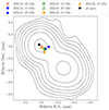 |
Fig. 7. Location of the radio core with respect to the 43-GHz one, overlaid on the 43-GHz map from the first observing epoch. Error bars are omitted for clarity. The average location to the central supermassive black hole is marked with a black dot. |
Based on the core shift measurement, we derived the equipartition magnetic field strengths 1 pc from the SMBH (Zdziarski et al. 2015), which are 1.91 ± 0.11 G for the first, 1.57 ± 0.17 G for the second, and 1.79 ± 0.16 G for the third epoch. These magnetic field strengths are close to the ones derived for the MOJAVE sample (Pushkarev et al. 2012) and by Zamaninasab et al. (2014) for AGN below redshift 2.43 and 2.37, respectively. Non-equipartition magnetic field strengths 1 pc from the SMBH are 324.7 ± 156.3 G, 104.9 ± 82.7 G, and 341.9 ± 225.2 G for the first, second, and third epochs, respectively. Extrapolating the average  to 5 rg, we measure
  G, a value significantly larger than the B ∼ 1 − 30 G reported for M 87 on horizon scales (Event Horizon Telescope Collaboration 2021).
Brightness temperatures as a function of the projected distance from the core can identify the dominant energy loss mechanism leading to the flux decay of jet components (Lobanov & Zensus 1999; Jorstad et al. 2005; Burd et al. 2022). According to the shock-in-jet model described by Marscher & Gear (1985), where an adiabatically expanding shock travels downstream in the jet, the main evolutionary stages the component goes through are characterized by Compton, synchrotron and adiabatic losses. In this scenario, brightness temperatures decay as power-laws, Tb, jet ∝ d−ϵ, where d is the distance of the jet component from the core, and ϵ is the power-law index, as the shock moves further away from the core (Schinzel et al. 2012; Kravchenko et al. 2016). In the case of TXS 1508+572, jet brightness temperatures can be described with power-law indices of 3.1 ± 0.6 at 15 GHz, −0.3 ± 1.11 at 22 GHz, and −1.7 ± 0.3 at 43 GHz (see Fig. 8). Tb gradients derived for 28 sources at 43 GHz by Burd et al. (2022) range from −3.19 to −1.23, with an average of −2.07, so our 43-GHz power-law index is consistent with these values. This Tb gradient places the jet of TXS 1508+572 in the Compton loss stage. The inverted and flat gradients at 15 and 22 GHz might be explained via the ongoing activity in the source. We suggest that the γ-ray activity observed in February 2022 is caused by a shock-shock interaction in the jet region of TXS 1508+572 and new plasma flowing through the C1 and C2 components. A similar phenomenon was observed in the blazar CTA 102 by Fromm et al. (2011) when a new shock wave traveled through a stationary re-collimation shock.
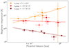 |
Fig. 8. Jet brightness temperature as a function of projected distance from the core. Solid lines represent power-law fits to the Tb, obs measurements at each frequency. |
5. Summary
After exhibiting a bright γ-ray flare, we started an intensive multi-wavelength follow-up campaign of the early-Universe blazar TXS 1508+572. To our knowledge, this is the first attempt at such observations of a flaring high-redshift AGN. While Paper I discusses the multi-wavelength properties of the source based on the quasi-simultaneous data we collected, here we focused on the VLBI observations included in our monitoring.
The present study of TXS 1508+572 extends our knowledge on the evolution of jet geometry and kinematics in high-redshift AGN. Our hybrid images reveal a compact core-jet structure on parsec scales (see Fig. 3). This morphology is affected by the γ-ray flare, as we recover changes in source structure and brightness on the timescale of months. Jet proper motion values of 0.12 − 0.27 mas yr−1 are recovered, corresponding to superluminal speeds of 14.3 − 32.2 c. This result is comparable to the high Lorentz factors of 20 used to model the SED in Paper I, and is consistent with maximum apparent speeds assuming Γ = 20 in the (μ − z) relation for high-redshift AGN (Zhang et al. 2022). We trace back the ejection time of the jet component to be between 2016 and 2019, during which TXS 1508+572 was in an elevated state in the γ-rays. This means that the jet component was not ejected as a result of the high-energy flare in 2022 February.
Using our multi-frequency data, we measured the distance to the central engine based on the core shift. The distance to the jet apex stays consistent within the measurement errors throughout our observations. On average, the central engine is located 46.1 ± 2.3 μas or 0.32 ± 0.02 pc from the 43-GHz VLBI core. Under the equipartition assumption, which is supported by our brightness temperature measurements in the presence of Doppler boosting, we measure  of 1.91 ± 0.11 G, 1.57 ± 0.17 G, and 1.79 ± 0.16 G for the three epochs. Low to intermediate redshift AGN also exhibit similar values of
  (Pushkarev et al. 2012; Zamaninasab et al. 2014).
  values are significantly higher than this, with 324.7 ± 156.3 G, 104.9 ± 82.7 G, and 341.9 ± 225.2 G for the consecutive epochs.
We note that even though we do not observe any brightening in the jet that would be clearly associated with the γ-ray flare of 2022, there might be a traveling disturbance, such as a density enhancement, that was not emitting much at radio waves but affected the position of the apparent cores at different frequencies during the 2022.67 epoch. This scenario coherently explains our kinematics and core shift measurements. Based on our analysis, we propose that the activity was caused by a shock-shock interaction between the already existing jet component of TXS 1508+572 and new plasma flowing through this region.
The data is available at: https://telamon.astro.uni-wuerzburg.de/
Acknowledgments
The authors thank the anonymous referee for useful comments that helped to improve the manuscript. The data were obtained at VLBA within the proposal BG281. The National Radio Astronomy Observatory is a facility of the National Science Foundation operated under cooperative agreement by Associated Universities, Inc. This work made use of the Swinburne University of Technology software correlator, developed as part of the Australian Major National Research Facilities Programme and operated under license. This research was supported through a PhD grant from the International Max Planck Research School (IMPRS) for Astronomy and Astrophysics at the Universities of Bonn and Cologne. This publication is part of the M2FINDERS project which has received funding from the European Research Council (ERC) under the European Union’s Horizon2020 Research and Innovation Programme (grant agreement No. 101018682). F.E., J.H., M.K., and F.R. acknowledge support from the Deutsche Forschungsgemeinschaft (DFG, grants 447572188, 434448349, 465409577).
References
- Abdollahi, S., Acero, F., Ackermann, M., et al. 2020, ApJS, 247, 33 [Google Scholar]
- Ackermann, M., Ajello, M., Baldini, L., et al. 2017, ApJ, 837, L5 [CrossRef] [Google Scholar]
- Aharonian, F. A. 2002, MNRAS, 332, 215 [Google Scholar]
- An, T., Mohan, P., Zhang, Y., et al. 2020, Nat. Commun., 11, 143 [Google Scholar]
- An, T., Wang, A., Zhang, Y., et al. 2022, MNRAS, 511, 4572 [NASA ADS] [CrossRef] [Google Scholar]
- Atwood, W. B., Abdo, A. A., Ackermann, M., et al. 2009, ApJ, 697, 1071 [CrossRef] [Google Scholar]
- Blandford, R. D., & Königl, A. 1979, ApJ, 232, 34 [Google Scholar]
- Bloemen, H., Bennett, K., Blom, J. J., et al. 1995, A&A, 293, L1 [NASA ADS] [Google Scholar]
- Böttcher, M., Reimer, A., Sweeney, K., et al. 2013, ApJ, 768, 54 [NASA ADS] [CrossRef] [Google Scholar]
- Burd, P. R., Kadler, M., Mannheim, K., et al. 2022, A&A, 660, A1 [NASA ADS] [CrossRef] [EDP Sciences] [Google Scholar]
- Cheung, C. C. 2004, ApJ, 600, L23 [NASA ADS] [CrossRef] [Google Scholar]
- Cohen, M. H., Barthel, P. D., Pearson, T. J., et al. 1988, ApJ, 329, 1 [NASA ADS] [CrossRef] [Google Scholar]
- Conway, J. E., & Murphy, D. W. 1993, ApJ, 411, 89 [NASA ADS] [CrossRef] [Google Scholar]
- Deller, A. T., Tingay, S. J., Bailes, M., et al. 2007, PASP, 119, 318 [NASA ADS] [CrossRef] [Google Scholar]
- Deller, A. T., Brisken, W. F., Phillips, C. J., et al. 2011, PASP, 123, 275 [Google Scholar]
- Eppel, F., Kadler, M., Heßdörfer, J., et al. 2024, A&A, 684, A11 [NASA ADS] [CrossRef] [EDP Sciences] [Google Scholar]
- Event Horizon Telescope Collaboration (Akiyama, K., et al.) 2019, ApJ, 875, L1 [Google Scholar]
- Event Horizon Telescope Collaboration (Akiyama, K., et al.) 2021, ApJ, 910, L13 [Google Scholar]
- Frey, S., Gurvits, L. I., Kellermann, K. I., et al. 1997, A&A, 325, 511 [NASA ADS] [Google Scholar]
- Frey, S., Paragi, Z., Fogasy, J. O., et al. 2015, MNRAS, 446, 2921 [CrossRef] [Google Scholar]
- Fromm, C. M., Perucho, M., Ros, E., et al. 2011, A&A, 531, A95 [NASA ADS] [CrossRef] [EDP Sciences] [Google Scholar]
- Gabányi, K. É., Belladitta, S., Frey, S., et al. 2023, PASA, 40, e004 [CrossRef] [Google Scholar]
- Ghisellini, G., Della Ceca, R., Volonteri, M., et al. 2010, MNRAS, 405, 387 [NASA ADS] [Google Scholar]
- Ghisellini, G., Haardt, F., Della Ceca, R., et al. 2013, MNRAS, 432, 2818 [NASA ADS] [CrossRef] [Google Scholar]
- Gokus, A., Kreter, M., Kadler, M., et al. 2022, ATel, 15202, 1 [NASA ADS] [Google Scholar]
- Gokus, A., Böttcher, M., Errando, M., et al. 2024, ApJ, Accepted [arXiv:2406.07635] [Google Scholar]
- Greisen, E. W. 2003, Astrophys. Space Sci. Lib., 285, 109 [NASA ADS] [Google Scholar]
- Gurvits, L. I. 2000, Perspectives on Radio Astronomy: Science with Large Antenna Arrays, 183 [Google Scholar]
- Gurvits, L. I., Frey, S., Krezinger, M., et al. 2023, IAU Symp., 375, 86 [Google Scholar]
- Hirotani, K. 2005, ApJ, 619, 73 [Google Scholar]
- Homan, D. C., Kadler, M., Kellermann, K. I., et al. 2009, ApJ, 706, 1253 [NASA ADS] [CrossRef] [Google Scholar]
- Homan, D. C., Lister, M. L., Kovalev, Y. Y., et al. 2015, ApJ, 798, 134 [Google Scholar]
- Hook, I. M., McMahon, R. G., Patnaik, A. R., et al. 1995, MNRAS, 273, L63 [NASA ADS] [Google Scholar]
- Jolley, E. J. D., & Kuncic, Z. 2008, MNRAS, 386, 989 [NASA ADS] [CrossRef] [Google Scholar]
- Jorstad, S. G., Marscher, A. P., Lister, M. L., et al. 2005, AJ, 130, 1418 [Google Scholar]
- Kappes, A., Burd, P. R., Kadler, M., et al. 2022, A&A, 663, A44 [NASA ADS] [CrossRef] [EDP Sciences] [Google Scholar]
- Kellermann, K. I., Vermeulen, R. C., Zensus, J. A., et al. 1999, New Astron. Rev., 43, 757 [CrossRef] [Google Scholar]
- Kovalev, Y. Y., Kellermann, K. I., Lister, M. L., et al. 2005, AJ, 130, 2473 [Google Scholar]
- Kravchenko, E. V., Kovalev, Y. Y., Hovatta, T., & Ramakrishnan, V. 2016, MNRAS, 462, 2747 [NASA ADS] [CrossRef] [Google Scholar]
- Kreter, M., Gokus, A., Krauss, F., et al. 2020, ApJ, 903, 128 [NASA ADS] [CrossRef] [Google Scholar]
- Krezinger, M., Perger, K., Gabányi, K. É., et al. 2022, ApJS, 260, 49 [NASA ADS] [CrossRef] [Google Scholar]
- Lampton, M., Margon, B., & Bowyer, S. 1976, ApJ, 208, 177 [Google Scholar]
- Lisakov, M. M., Kovalev, Y. Y., Savolainen, T., et al. 2017, MNRAS, 468, 4478 [NASA ADS] [CrossRef] [Google Scholar]
- Lister, M. L., Homan, D. C., Kellermann, K. I., et al. 2021, ApJ, 923, 30 [NASA ADS] [CrossRef] [Google Scholar]
- Lobanov, A. P. 1998, A&A, 330, 79 [NASA ADS] [Google Scholar]
- Lobanov, A. P., & Zensus, J. A. 1999, ApJ, 521, 509 [Google Scholar]
- Marcaide, J. M., & Shapiro, I. I. 1984, ApJ, 276, 56 [Google Scholar]
- Marscher, A. P., & Gear, W. K. 1985, ApJ, 298, 114 [Google Scholar]
- Niinuma, K., Kino, M., Doi, A., et al. 2015, ApJ, 807, L14 [NASA ADS] [CrossRef] [Google Scholar]
- Orienti, M., D’Ammando, F., Giroletti, M., et al. 2014, MNRAS, 444, 3040 [CrossRef] [Google Scholar]
- O’Sullivan, S. P., Gabuzda, D. C., & Gurvits, L. I. 2011, MNRAS, 415, 3049 [Google Scholar]
- Padovani, P., & Giommi, P. 1995, ApJ, 444, 567 [NASA ADS] [CrossRef] [Google Scholar]
- Paliya, V. S., Ajello, M., Ojha, R., et al. 2019, ApJ, 871, 211 [NASA ADS] [CrossRef] [Google Scholar]
- Pearson, T. J., & Readhead, A. C. S. 1988, ApJ, 328, 114 [Google Scholar]
- Perger, K., Frey, S., Gabányi, K. É., et al. 2018, MNRAS, 477, 1065 [NASA ADS] [CrossRef] [Google Scholar]
- Péroux, C., Storrie-Lombardi, L. J., McMahon, R. G., et al. 2001, AJ, 121, 1799 [CrossRef] [Google Scholar]
- Plavin, A. V., Kovalev, Y. Y., Pushkarev, A. B., et al. 2019, MNRAS, 485, 1822 [NASA ADS] [CrossRef] [Google Scholar]
- Pushkarev, A. B., Hovatta, T., Kovalev, Y. Y., et al. 2012, A&A, 545, A113 [NASA ADS] [CrossRef] [EDP Sciences] [Google Scholar]
- Readhead, A. C. S. 1994, ApJ, 426, 51 [Google Scholar]
- Salvatelli, V., Marchini, A., Lopez-Honorez, L., et al. 2013, Phys. Rev. D, 88, 023531 [NASA ADS] [CrossRef] [Google Scholar]
- Schinzel, F. K., Lobanov, A. P., Taylor, G. B., et al. 2012, A&A, 537, A70 [NASA ADS] [CrossRef] [EDP Sciences] [Google Scholar]
- Schneider, D. P., Hall, P. B., Richards, G. T., et al. 2007, AJ, 134, 102 [NASA ADS] [CrossRef] [Google Scholar]
- Shepherd, M. C. 1997, ASP Conf. Ser., 125, 77 [Google Scholar]
- Titov, O., Frey, S., Melnikov, A., et al. 2023, AJ, 165, 69 [NASA ADS] [CrossRef] [Google Scholar]
- Urry, C. M., & Padovani, P. 1995, PASP, 107, 803 [NASA ADS] [CrossRef] [Google Scholar]
- Veres, P., Frey, S., Paragi, Z., et al. 2010, A&A, 521, A6 [NASA ADS] [CrossRef] [EDP Sciences] [Google Scholar]
- Vermeulen, R. C., & Cohen, M. H. 1994, ApJ, 430, 467 [NASA ADS] [CrossRef] [Google Scholar]
- Volonteri, M. 2010, A&ARv, 18, 279 [Google Scholar]
- Weaver, Z. R., Jorstad, S. G., Marscher, A. P., et al. 2022, ApJS, 260, 12 [NASA ADS] [CrossRef] [Google Scholar]
- Zamaninasab, M., Clausen-Brown, E., Savolainen, T., et al. 2014, Nature, 510, 126 [CrossRef] [Google Scholar]
- Zdziarski, A. A., Sikora, M., Pjanka, P., et al. 2015, MNRAS, 451, 927 [CrossRef] [Google Scholar]
- Zhang, Y., An, T., & Frey, S. 2020, Sci. Bull., 65, 525 [NASA ADS] [CrossRef] [Google Scholar]
- Zhang, Y., An, T., Frey, S., et al. 2022, ApJ, 937, 19 [NASA ADS] [CrossRef] [Google Scholar]
Appendix A: Additional figures and tables
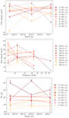 |
Fig. A.1. Light curves, spectra, and brightness temperatures of the core and jet components of TXS 1508+572. |
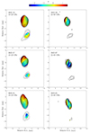 |
Fig. A.2. Spectral index maps between 15, 22 and 43 GHz. |
Summary of image parameters.
Properties of modelfit components.
Appendix B: Multi-frequency kinematic fit
Here we present a multi-frequency kinematic analysis of the two jet components whose positions were aligned based on the core shift measurement (see Sect. 3.2). The component distances and the best fit functions are shown in Fig. B.1. Our data is well described with a linear fit which reveals apparent component speed of μC1 = 0.16 ± 0.07 mas/yr and μC2 = 0.20 ± 0.08 mas/yr.
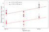 |
Fig. B.1. Kinematics of the jet components C1 (red circles) and C2 (dark red squares), with their positions aligned based on the core shift measurement. |
However, the amount of data available for kinematic estimates is not sufficient to justify higher orders of trajectory fit, and our overall conclusions are not strongly dependent on the linearity of the apparent trajectory. In addition, according to the methodology established for AGN monitoring data Homan et al. (2009), component acceleration is only analyzed if a given jet feature is robustly detected in at least ten observing epochs. Linear fits are more suitable to determine the component speed and ejection time. Nevertheless, our data presented here would be a useful set of future study of kinematics which might favor a higher order of trajectory fit.
All Tables
All Figures
|
Fig. 1. Radio light curve of TXS 1508+572 observed with the Effelsberg 100-m telescope after the γ-ray flare (dashed black line). The VLBI observations are marked with black dotted lines. |
| In the text | |
|
Fig. 2. Left panel: (u, v) coverage of the 43-GHz VLBA and EF (grey) and the 86-GHz VLBA and GBT (black) observations, plotting the fringe detections. Right panel: self-calibrated amplitude and phase of the 86-GHz data set. |
| In the text | |
|
Fig. 3. Clean images of TXS 1508+572 at 15, 22, and 43 GHz. The observations were carried out in 2022 March, September, and in 2023 January (see Table 1). Image properties are summarized in Table A.1. Contours and colors represent the brightness distribution of the parsec-scale structure of the object. The images are aligned based on the core shift measurement. |
| In the text | |
|
Fig. 4. 43 and 86 GHz image of TXS 1508+572 observed with the VLBA+EF (43 GHz, left) and VLBA+GBT (86 GHz, right). Lowest contours are at 0.53 and 1.37 mJy beam−1, and increase as a factor of two. Positions of the modelfit components are overlaid as black circles. |
| In the text | |
|
Fig. 5. Kinematics of the jet component at 15 (orange circles), 22 (red squares), and 43 GHz (dark red triangles) following the γ-ray flare. Jet speeds are listed in the text in Sect. 3. The positional errors are assumed to be one fifth of the beam minor axis. Note the systematic offset of the position of both jet components at the higher frequencies, which is roughly consistent with the core shift determined in Sect. 4.3. |
| In the text | |
|
Fig. 6. Evolution of the core shift measured throughout the first (gold), second (red), and third (purple) VLBI epochs. The distance to the jet apex (r0) is shown in the legend for each of the three epochs. |
| In the text | |
|
Fig. 7. Location of the radio core with respect to the 43-GHz one, overlaid on the 43-GHz map from the first observing epoch. Error bars are omitted for clarity. The average location to the central supermassive black hole is marked with a black dot. |
| In the text | |
|
Fig. 8. Jet brightness temperature as a function of projected distance from the core. Solid lines represent power-law fits to the Tb, obs measurements at each frequency. |
| In the text | |
|
Fig. A.1. Light curves, spectra, and brightness temperatures of the core and jet components of TXS 1508+572. |
| In the text | |
|
Fig. A.2. Spectral index maps between 15, 22 and 43 GHz. |
| In the text | |
|
Fig. B.1. Kinematics of the jet components C1 (red circles) and C2 (dark red squares), with their positions aligned based on the core shift measurement. |
| In the text | |
Current usage metrics show cumulative count of Article Views (full-text article views including HTML views, PDF and ePub downloads, according to the available data) and Abstracts Views on Vision4Press platform.
Data correspond to usage on the plateform after 2015. The current usage metrics is available 48-96 hours after online publication and is updated daily on week days.
Initial download of the metrics may take a while.