| Issue |
A&A
Volume 689, September 2024
|
|
|---|---|---|
| Article Number | A266 | |
| Number of page(s) | 9 | |
| Section | Extragalactic astronomy | |
| DOI | https://doi.org/10.1051/0004-6361/202450150 | |
| Published online | 20 September 2024 | |
Long gamma-ray burst light curves as the result of a common stochastic pulse–avalanche process
1
Department of Physics and Earth Science, University of Ferrara, Via Saragat 1, 44122 Ferrara, Italy
2
INAF – Osservatorio di Astrofisica e Scienza dello Spazio di Bologna, Via Piero Gobetti 101, 40129 Bologna, Italy
3
INFN – Sezione di Ferrara, Via Saragat 1, 44122 Ferrara, Italy
4
INAF – Osservatorio Astronomico di Capodimonte, Salita Moiariello 16, 80131 Napoli, Italy
5
Dipartimento di Fisica “E. Pancini”, Università di Napoli “Federico II”, Via Cinthia 21, 80126 Napoli, Italy
6
INAF, Osservatorio Astronomico d’Abruzzo, Via Mentore Maggini snc, 64100 Teramo, Italy
7
Department of Physics, University of Cagliari, SP Monserrato-Sestu, km 0.7, 09042 Monserrato, Italy
8
Ioffe Institute, Politekhnicheskaya 26, 194021 St. Petersburg, Russia
Received:
27
March
2024
Accepted:
27
June
2024
Abstract
Context. The complexity and variety exhibited by the light curves of long gamma-ray bursts (GRBs) enclose a wealth of information that has not yet been fully deciphered. Despite the tremendous advance in the knowledge of the energetics, structure, and composition of the relativistic jet that results from the core collapse of the progenitor star, the nature of the inner engine, how it powers the relativistic outflow, and the dissipation mechanisms remain open issues.
Aims. A promising way to gain insights is describing GRB light curves as the result of a common stochastic process. In the Burst And Transient Source Experiment (BATSE) era, a stochastic pulse avalanche model was proposed and tested through the comparison of ensemble-average properties of simulated and real light curves. Here our aim was to revive and further test this model.
Methods. We applied it to two independent datasets, BATSE and Swift/BAT, through a machine learning approach: the model parameters are optimised using a genetic algorithm.
Results. The average properties were successfully reproduced. Notwithstanding the different populations and passbands of both datasets, the corresponding optimal parameters are interestingly similar. In particular, for both sets the dynamics appear to be close to a critical state, which is key to reproducing the observed variety of time profiles.
Conclusions. Our results propel the avalanche character in a critical regime as a key trait of the energy release in GRB engines, which underpins some kind of instability.
Key words: methods: statistical / gamma-ray burst: general
Corresponding author; This email address is being protected from spambots. You need JavaScript enabled to view it. .
© The Authors 2024
 Open Access article, published by EDP Sciences, under the terms of the Creative Commons Attribution License (https://creativecommons.org/licenses/by/4.0), which permits unrestricted use, distribution, and reproduction in any medium, provided the original work is properly cited.
This article is published in open access under the Subscribe to Open model. This email address is being protected from spambots. You need JavaScript enabled to view it. to support open access publication.
1. Introduction
Gamma-ray bursts (GRBs) are the most powerful explosions on stellar scale in the Universe. At least two kinds of progenitors are known: (a) the ‘collapsar’ (Woosley 1993; Paczyński 1998; MacFadyen & Woosley 1999), which is a hydrogen-stripped massive star whose core collapses to a compact object, and that launches a relativistic (Γ ∼ 102–103) jet, and (b) the merger of a compact binary (Eichler et al. 1989; Paczynski 1991; Narayan et al. 1992), where at least one of the two objects is supposed to be a neutron star (NS), and that also results in a short-lived relativistic jet (see Kumar & Zhang 2015; Zhang 2018 for recent reviews). There are alternative models to the collapsar, such as the binary-driven hypernova model (BdHN; Rueda & Ruffini 2012; Becerra et al. 2019), in which the final collapse of a CO core of a massive star can trigger the collapse of a companion neutron star. Most GRBs with a progenitor of type (a) manifest themselves as long GRBs (LGRBs), lasting longer than ∼2 s1, while those with a type (b) progenitor usually exhibit a subsecond spike occasionally followed by weak long-lasting emission (Norris & Bonnell 2006), and are commonly referred to as short GRBs (SGRBs). Actually, the emerging picture is more complicated, as shown by the increasing number of cases with deceptive time profiles found in both classes (Gehrels et al. 2006; Rastinejad et al. 2022; Gompertz et al. 2023; Yang et al. 2022; Troja et al. 2022; Ahumada et al. 2021; Zhang et al. 2021; Rossi et al. 2022; Levan et al. 2023, 2024).
The nature of the dissipation mechanism that is responsible for the GRB prompt emission is still an open issue. The great variety observed in the light curves (LCs) of LGRBs is thought to be the result of the variability imprinted on the relativistic outflow by the inner engine left over by the collapsar, either a millisecond magnetised NS or a black hole (BH), along with the effects of the propagation of the jet within the stellar envelope (e.g. Morsony et al. 2010; Geng et al. 2016; Gottlieb et al. 2020a, 2020b, 2021a; Gottlieb et al. 2021b), although some models ascribe the possible presence of subsecond variability to magnetic reconnection events taking place at larger radii (Zhang & Yan 2011). Some correlations were found between the variability and minimum variability timescales on the one hand, as defined in a number of ways, and the luminosity and initial Lorentz factor of the outflow on the other hand (see e.g. Camisasca et al. 2023 and references therein). However, apart from the study of average and of individual Fourier power density spectra of GRBs (Beloborodov et al. 1998; Guidorzi et al. 2012, 2016; Dichiara et al. 2013), the study of the waiting time distribution between pulses (Ramirez-Ruiz et al. 2001; Nakar & Piran 2002; Quilligan et al. 2002; Guidorzi et al. 2015), and the distribution of the number of peaks per GRB (Guidorzi et al. 2024), little progress has been made in deciphering and characterising the variety of LGRB LCs within a unifying scheme that could explain the large diversity (in terms of duration, number of pulses, distribution of energy, and waiting times between pulses) and relate it to other key properties.
Given the observed erratic behaviour of GRB LCs, two primary hypotheses can be identified: (i) the apparent lack of periodicity or distinct patterns, which precludes an easy classification and the prediction of GRB LCs, may originate from deterministic, non-linear, and possibly chaotic processes, and (ii) the energy release mechanism might be inherently stochastic. While hypothesis (i) has been explored in previous studies (e.g. Greco et al. 2011) and remains plausible, our work focuses instead on scenario (ii). A stochastic character is also naturally invoked in the presence of turbulence. For instance, magnetised GRB outflows can experience turbulent magnetic reconnection episodes (Lazarian & Vishniac 1999).
Recent investigations found possible evidence that GRB engines emit as self-organised critical (SOC) systems (Wang & Dai 2013; Yi et al. 2017; Lyu et al. 2020; Wei 2023; Li & Yang 2023; Maccary et al. 2024), in which energy is released through avalanches whenever the system naturally reaches a critical point. However, the interpretation is not straightforward since SOC dynamics is usually invoked for systems that are continuously fed by some energy input and are not characterised by the kind of irreversible evolution expected for a GRB inner engine. A successful description of the inner engine variability would help to constrain the mechanism that powers the jetted outflow in GRBs and, ultimately, the nature of the compact object. Furthermore, it would provide the community with a reliable tool to simulate credible GRB LCs as they would be measured by future experiments, avoiding the pitfalls of using noisy real LCs (e.g. Sanna et al. 2020).
In this respect, an interesting attempt was laid out by Stern & Svensson (1996, hereafter SS96) in the Compton Gamma-Ray Observatory era (CGRO; 1991–2000) in the GRB catalogue of one of its experiments, the Burst And Transient Source Experiment (BATSE). These authors proposed a common stochastic process built on a pulse avalanche mechanism, and tried to reproduce some of the observed distributions of BATSE GRB LCs. At that time, the cosmological distances of GRBs and the nature of the progenitors of the two classes were yet to be firmly established, with the first afterglow discoveries starting in 1997 (Costa et al. 1997). By manually guessing the values of the seven model parameters, SS96 came up with a process operating in a nearly critical regime and capable of reproducing the variety of observed GRB LCs, with respect to the chosen metrics. This approach of simulating GRB LCs was adopted in Greiner et al. (2022) to assess localisation capabilities of a proposed network of GRB detectors on the global navigation satellite system Galileo G2.
The SS96 model represents an interesting attempt to capture essential aspects of the way energy is dissipated over time beyond a generic and rather uninformative attribute such as ‘random’ used to describe the sequence of peaks and pulses. The core mechanism of this model is the avalanche through which energy is released as a runaway process triggered by some kind of instability. Some initial episodes of energy release, which turn up as major pulses in the LC (called ‘parent pulses’), can further give rise to ‘child pulses’ and so on, until the process becomes subcritical.
A possibility that could give rise to an avalanche process similar to the one underpinning the SS96 model is given by magneto-rotational and/or gravitational instabilities in the hyperaccreting disc of the left-over compact object, which then cause fragmentation (also proposed by Perna et al. 2006 to explain GRB X-ray flares). Child pulses could result from further fragmentation of a parent episode, from viscous instabilities that form clumps, which can imprint a branching character (e.g. Kawanaka et al. 2013; Shahamat et al. 2021), or from current-driven instabilities as in the Poynting-flux dominated outflow described by Lyutikov (2003). Another possibility is related to the runaway character of the magnetic reconnection events that are envisaged in the Internal-Collision-induced MAgnetic Reconnection and Turbulence model (ICMART; Zhang & Yan 2011).
In the big data era, advanced statistical and machine learning (ML) techniques applied to astrophysics have become routine (see e.g. Feigelson et al. 2021 for a review). In this paper our aim is to verify and improve the results obtained by SS96 on the BATSE data and, for the first time, apply their model to a sample from another detector operating in a softer energy band, such as the Burst Alert Telescope (BAT; Barthelmy et al. 2005) on board the Neil Gehrels Swift Observatory (Gehrels et al. 2004). Specifically, we want to optimise the model parameters using a genetic algorithm (GA; Rojas 1996).
A similar technique, in which the parameters of a physical model were optimised through the application of a GA, was recently applied by Vargas et al. (2022) to model the shock propagation in the supernova SN2014C progenitor star and ejecta. The GA was used to optimise a hydrodynamic and radiation transfer model.
Unlike SS96, we restricted our analysis to LGRBs, whose progenitor is thought to be a collapsar, to preserve as much as possible the homogeneity of the putative GRB inner engines. For ∼30% of the Swift sample with measured redshift, in principle it is possible to carry out the same analysis in the GRB rest frame. However, we did not consider this option, since the cosmological dilation correction by (1 + z) is partly counteracted by other energy-dependent effects, which make the final correction milder and less obvious (see Camisasca et al. 2023 and references therein for a detailed explanation).
In this paper we report the main results and implications. A companion and more ML-oriented paper will report all the technical details. The present work is organised as follows. In Sect. 2 we describe the data analysis and sample selection, while in Sect. 3 we illustrate the methods underpinning the avalanche model and the implementation of the genetic algorithm. In Sect. 4 we report the results. We discuss the results and lay out our conclusions in Sect. 5.
2. Data analysis
2.1. Sample selection
From the BATSE 4B catalogue (Paciesas et al. 1999) we took the 64 ms time profiles that were made available by the BATSE team2. Observed with the eight BATSE large area detectors (LADs), these data are the result of a concatenation of three standard BATSE types, DISCLA, PREB, and DISCSC, available in four energy channels: 25–55, 55–110, 110–320, and > 320 keV. We used the total passband LCs. For each GRB the background was interpolated with polynomials of up to fourth degree, as prescribed by the BATSE team. In our analysis we used the background-subtracted LCs.
From an initial sample of 2024 GRBs we selected only those that satisfy the following requirements:
-
T90 > 2 s, that is, only LGRBs;
-
data available for at least 150 s after the brightest peak;
-
signal-to-noise ratio (S/N) of the total net counts within the duration of the event greater than 70.
In order to estimate the S/N, following SS96, rather than the commonly used T90, we used as a proxy of the GRB duration the time interval from the first to the last time bin whose counts exceed the threshold of 20% of the peak counts, henceforth called T20%. Before evaluating the T20%, the LCs were first convolved with a Savitzky-Golay smoothing filter (Savitzky & Golay 1964), using a second-order interpolating polynomial, and a moving window of size T90/15. Accordingly, we defined the S/N of a GRB as the sum of the net counts in the whole T20% interval, divided by the corresponding error. The value of the S/N threshold was the result of a trade-off between the number of GRBs and the statistical quality of the LCs in the sample. Furthermore, the T20% was also used to compute the duration distribution of the LCs (Sect. 2.2).
We ended up with 585 LGRBs satisfying the aforementioned properties. Hereafter, this is referred to as the BATSE sample.
As a second dataset, we considered the GRBs detected by Swift/BAT from January 2005 to November 2023 and covered in burst mode. We used the total 15–150 keV passband LCs, with 64 ms bin time; these were extracted as mask-weighted background-subtracted LCs, following the standard procedure recommended by the BAT team3. From an initial sample of 1389 GRBs observed in burst mode, 531 passed the selection based on the same criteria adopted for BATSE, except for the value of the S/N threshold, which was lowered to 15 to obtain a sample of comparable size to the BATSE sample, but still ensuring the required statistical quality. Hereafter, this is referred to as the Swift sample.
2.2. Statistical metrics
We considered the following four metrics, which were also used by SS96:
-
Average peak-aligned post-peak time profile (Mitrofanov 1996), in the time range 0–150 s after the brightest peak. It is evaluated by averaging the normalised count rate of all the LCs in the sample (i.e. ⟨F/Fp⟩, Fp being the peak count rate). Further details are given in Stern (1996);
-
Average peak-aligned third moment of post-peak time profiles ⟨(F/Fp)3⟩, evaluated analogously to the first moment;
-
Average auto-correlation function (ACF). For both data samples the ACF is corrected for the counting statistics noise as in Link et al. (1993) and is computed in the 0–150 s interval;
-
T20% distribution, with T20% used as a proxy of the duration.
As in SS96, these four metrics were used to evaluate the degree of similarity between the real and the simulated LCs.
3. Methods
3.1. Light curve simulations
The stochastic process conceived by SS96 belongs to the class known as ‘branching’ processes, which describe the development of a population whose members reproduce according to some random process (Harris 1963). The process by SS96 aims to mimic the temporal properties of GRBs and works as a pulse avalanche, which is a linear Markov process. We outline its key features below, and refer to SS96 for more details. The SS96 model is based on the assumptions that:
-
GRB LCs can be viewed as distinct random realisations of a common stochastic process, within narrow parameter ranges;
-
the stochastic process should be scale invariant in time;
-
it operates close to a critical state.
With this model, each LC consists of a series of spontaneous primary (or parent) pulses, each of which can give rise to secondary (or child) pulses, which can then recursively spawn other generations of child pulses until the process reaches subcritical conditions and stops. Each pulse, which acts as a building block, is described by a Gaussian rise followed by a simple exponential decay:
 (1)
(1)
Here τ is roughly the pulse width, tp is the peak time, A is the amplitude, and we assume τr = τ/2 (Norris et al. 1996). Differently from SS96, we do not sample A from a uniform distribution 𝒰[0, 1]; rather, for each GRB we sample the value Amax from the distribution of the peak count rates of the real observed LCs, and then the amplitude of each pulse composing that LC is sampled from 𝒰[0, Amax].
The model is described by seven parameters:
-
μ0 rules the number μs of spontaneous initial pulses per GRB, which is sampled from a Poisson distribution with μ0 as expected value:
 (2)
(2) -
μ rules the number of child pulses μc generated by each parent pulse, which is sampled from a Poisson distribution with μ as expected value:
 (3)
(3) -
α rules the delay Δt between a child and its parent. This delay is exponentially distributed, with e-folding time given by (ατ), where τ is the time constant of the child pulse:
 (4)
(4)Moreover, the spontaneous μs primary pulses are all assumed to be delayed with respect to a common invisible trigger event; the probability distribution of the delay t is exponentially distributed,
 (5)
(5)τ0 being the time constant of the primary pulse.
-
τmin and τmax define the boundaries for the constant τ0 of the initial spontaneous pulses and whose probability density function is p(τ0)∝1/τ0, equivalent to a uniform distribution of log τ0,
![Mathematical equation: $$ \begin{aligned} p (\log \tau _0) = \left[\log \tau _{\max }-\log \tau _{\min }\right]^{-1}, \end{aligned} $$](/articles/aa/full_html/2024/09/aa50150-24/aa50150-24-eq6.gif) (6)
(6)where τmin has to be shorter than the time resolution of the instrument. Varying τmax is equivalent to rescaling all average avalanche properties in time.
-
δ1 and δ2 define the boundaries, [δ1, δ2], of a uniform distribution assumed for the logarithm of the ratio between τ of the child and τp of its parent,
![Mathematical equation: $$ \begin{aligned} p[\log (\tau /\tau _p)] = \left|\delta _2 - \delta _1\right|^{-1}, \end{aligned} $$](/articles/aa/full_html/2024/09/aa50150-24/aa50150-24-eq7.gif) (7)
(7)with δ1 < 0, δ2 ≥ 0, and |δ1|> |δ2|.
Each of the μs spontaneous initial pulses gives rise to a pulse avalanche, acting as a parent, spawning another set of child pulses, in a recurrent way. The avalanche ends when it converges due to subcritical values of the model parameters. Finally, it is the superposition of the parents and all the generations of child pulses created during the avalanche that shapes the LC of an individual GRB.
The stochastic pulse avalanche model was used to simulate both BATSE and Swift/BAT LCs. The statistical noise depends on the total counts in each time bin, which requires the knowledge of the typical background count rate for a given instrument. For BATSE, which consisted of NaI(Tl) scintillators, we assumed a constant background rate of 2.9 cnt s−1 cm−2, which corresponds to the median of the distribution of the measured error rates. Each final simulated LC was the result of a Poisson realisation, assuming for each time bin the total counts (i.e. noise-free simulated profile plus background) as the expected value. Lastly, the background was removed.
Swift/BAT is a coded mask coupled with a CZT detection array. Its background-subtracted LCs are the result of the deconvolution of the detection with the pattern of the mask, so the rate in each time bin can be modelled as a Gaussian variable. To simulate BAT LCs, the rate of each time bin was sampled from a Gaussian distribution centred on the LC (noise-free) model obtained with the pulse avalanche model, and with standard deviation randomly sampled from the errors measured in the real Swift/BAT LCs.
All the simulations were conducted using an open-source Python4 implementation of the SS96 model. This code, developed by one of the authors, is publicly available in a GitHub repository5.
3.2. Genetic algorithm
In their work, SS96 proposed a set of values for the seven model parameters based on an educated guess. The optimisation of these parameters, however, is an ideal task for the ML techniques routinely used today.
Genetic algorithms are a specific type of algorithms in the larger family known as evolutionary algorithms (Russell & Norvig 2021; Rojas 1996; Aggarwal 2021; Hurbans 2020), where a Darwinian evolution process is simulated to find the parameters that maximise a function. In GAs, each solution to an optimisation problem can be seen as an individual, with the fitness of that individual being determined by the objective function value of the corresponding solution. These solutions are points in the domain of the function to be optimised. In our work, each individual was represented by a genome made of seven genes, which are the parameters of the SS96 model described in Sect. 3.1.
At each generation, a new set of individuals is created. Over time, the points belonging to the new generations gradually converge towards local maxima of the fitness function. In order to improve the overall fitness of the population over successive generations, GAs incorporate three fundamental processes: selection, crossover, and mutation.
The typical life cycle of a GA, made up of a succession of these generations, includes the following steps:
-
Population initialisation: Randomly generating a population of potential solutions;
-
Evaluating fitness: Assessing the quality of each individual by employing a fitness function that assigns scores to evaluate their fitness;
-
Parent selection: Choosing pairs of parents for reproduction based on their fitness score;
-
Offspring creation: Producing offspring by combining genetic information from parents, and introducing random mutations;
-
Generation advancement: Selecting individuals and offspring from the population to progress to the next generation.
Genetic algorithms are particularly useful in situations where there is no available information about the function’s gradient at the evaluated points. Indeed, GAs can effectively handle functions that are not continuous or differentiable (Rojas 1996).
3.3. Parameter optimisation
The GA was implemented using PyGAD6, an open-source Python library containing a collection of several ML algorithms (Gad 2023). We constrained the seven parameters of the model within the intervals shown in Table 1.
Region of exploration during the GA optimisation of the seven parameters of the SS96 stochastic model.
The GA evolved through a sequence of generations consisting of a population with Npop = 2000 individual sets of seven parameters. Each set of parameters, hereafter referred to as an individual, was then used to generate Ngrb = 2000 LCs. The very same three constraints mentioned in Sect. 2.1 and used for the selection of BATSE and Swift/BAT dataset were also applied on the simulated GRB LCs, the generated ones not satisfying such constraints being discarded. For each of the Npop individuals, we evaluated the same four metrics defined in SS96 over the corresponding Ngrb LCs (cf. Sect. 2.2), and compared them with the values obtained from the real datasets, by computing the L2 loss between these four observables. The final loss associated with a given individual was simply defined as the average of these four quantities, the fitness score being the inverse of this value.
Individuals were then ranked based on their loss. The next generation of individuals was obtained by mixing the genes (i.e. the values of the seven parameters) of the fittest individuals in the current generation. No individuals were automatically kept in the next generation; that is, we set the ‘elitism’ to zero7. The offspring was obtained by randomly sampling two individuals among the top 15% in the current generation and assigning to each gene the value of the seven parameters from one of the two parents, with equal probability.
Finally, we included the possibility for genetic random mutations to occur. During the mating step, each one of the seven parameters had a 4% probability of undergoing mutation, meaning that the value of the parameters was not inherited from one of the two parents; instead, it was randomly sampled from the exploration range of the parameter (Table 1). The optimisation process was stopped when convergence of the loss, and thus of the value of the seven parameters, was reached.
4. Results
In Table 2 we compare the values of the seven model parameters suggested in SS96 with the results of our GA optimisation on the BATSE and Swift training datasets. The final optimised values of the seven parameters are obtained as the median value for the whole population of the last GA generation. We also list the achieved values of the loss function evaluated on the training set (both in terms of best parameter configuration and by averaging on the last population) and on the test set (i.e. estimated by using 5000 newly simulated GRB LCs). At the bottom, we resolve the individual contribution of each component to the test loss.
Results of the GA optimisation on the BATSE and Swift datasets.
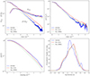 |
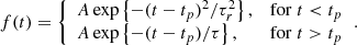
Fig. 1. Average distributions of real (blue), simulated GA-optimised (red), and simulated SS96 (green) BATSE GRB profiles, estimated on the test set (see Table 2). Top left: Average peak-aligned post-peak normalised time profile, together with the r.m.s. deviation of the individual peak-aligned time profiles, Frms ≡ [⟨(F/Fp)2⟩−⟨F/Fp⟩2]1/2. Top right: Average peak-aligned third moment test. Bottom left: Average ACF of the GRBs. Bottom right: Distribution of duration, measured at a level of 20% of the peak amplitude (T20%). In the top left and top right panels, both real and simulated averaged curves were smoothed with a Savitzky-Golay filter to reduce the effect of Poisson noise. In the bottom right panel, a Gaussian kernel convolution has been applied to both real and simulated distributions. |
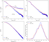 |
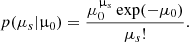
Fig. 2. Comparison between the real Swift/BAT dataset and the corresponding simulated dataset on the same four metrics defined for the BATSE dataset, analogously to Fig. 1. |
Figure 1 displays the comparison of the four observables, described in Sect. 2.2, between the real BATSE curves and simulated curves (test set). In particular, the panels show the average profiles obtained from the 585 useful BATSE events (blue), those estimated from 5000 simulated GRBs with optimised parameters (red), and those estimated from 5000 LCs simulated using the parameter values guessed by SS96 (green). Figure 2 shows the analogous comparison between the simulated and the real Swift/BAT curves.
We find excellent agreement for three out of the four metrics computed from the real and simulated BATSE LCs, in particular for the average post-peak time profile, its third moment, and the average auto-correlation, whose L2 loss values are smaller than the corresponding values estimated with SS96 non-optimised parameters, as can be seen from the bottom part of Table 2. For instance, the average ACF metric shows a relative improvement of ∼74% after the optimisation. The T20% distribution holds the largest contribution to the loss; however, it slightly improves the SS96 performance (∼8% relative improvement). Overall, compared with SS96, our GA-optimised results on the BATSE data better reproduce the observed distributions.
As can be inferred from Table 2, and graphically from Fig. 2, according to the loss function the avalanche model appears to work even better in the case of Swift data. The results on the average ACF and third moment of peak-aligned profiles are comparably good, whereas the average peak-aligned profile and duration distributions are significantly improved with respect to the BATSE case, with a relative loss decrease of ∼43% and ∼58%, respectively.
Notably, the two sets of best-fitting parameters obtained with BATSE and with Swift/BAT are very similar and, surprisingly, overall not too different from the values guessed by SS96. In Sect. 5 we discuss the relevance of this result in more detail.
The parameters for which our optimal values for both sets are somewhat different from those of SS96 are (δ1, δ2), τmax, and α. The first pair defines the dynamic range of the child-to-parent pulse duration ratio; our values turn into broader dynamical ranges than SS96, and, at variance with those authors, they admit the possibility of children lasting longer than parents, being δ2 > 0. While SS96 assumed τmax = 26 s as the maximum value for the duration of parent pulses, our optimised solution favours the possibility of longer parent pulses: 40.2 s for BATSE and 56.8 s for Swift/BAT. Finally, our best-fit values for α, which rules the time delay between parent and child, lean towards slightly shorter intervals than SS96.
As in SS96, Fig. 3 presents the comparison of four real BATSE time profiles with four simulated LCs of similar morphology and complexity, sampled from the test set, generated using the best-fitting set of BATSE model parameters given above. This qualitative plot shows the ability of the SS96 stochastic model to reproduce the different morphological classes of LCs discussed in the literature from the earliest observations (Fishman & Meegan 1995).
 |
Fig. 3. Four examples of as many classes of GRB LCs from the BATSE real sample (left) along with their trigger number, and the corresponding simulated sample (right). Following the same qualitative classification adopted by SS96, from top to bottom the four classes are single pulse, blending of some pulses, moderately structured, and highly erratic. At the top right of each subplot is shown the average error on the counts of the corresponding LC. |
5. Discussion and conclusions
For the first time in the GRB literature, here we developed and implemented an ML technique to optimise the parameters of a stochastic model capable of generating realistic GRB LCs from scratch. Our work confirmed the soundness of the insight by SS96: a simple toy model like the stochastic pulse avalanche model is able to generate populations of LCs, whose average behaviour closely resembles that of the real populations of BATSE and Swift/BAT LGRBs. With the implementation of GA, we found the two best-fitting sets of the seven parameters of the model that best reproduce the average behaviours of the two datasets, thus (i) progressing from the values from the original paper obtained via an educated guess to a real fit of the model on BATSE data, and (ii) applying it for the first time to an independent catalogue of GRB LCs such as Swift/BAT, whose data differ from BATSE in many aspects, as detailed below.
In light of our GA-optimised results on the BATSE data, the educated guess by SS96 turns out to be surprisingly good. In particular, the finding that μ, which is the average number of child-pulses generated by each parent-pulse, must be close to unity (our  vs. 1.20 of SS96) confirms the insightful Ansatz by SS96 that the model must operate very close to a critical regime (μ = 1), to account for the observed variety of GRB profiles. Interestingly, the same clue is also obtained in the GA-optimised parameters of the Swift/BAT sample. This result is far from obvious for three main reasons: (i) the passband of the two experiments is significantly different, with Swift/BAT profiles being softer and, as such, less spiky (e.g. Fenimore 1995; ii) the average S/N of the two sets is also remarkably different, with a minimum value of 70 for BATSE, to be compared with the poorer lower threshold of 15 for Swift/BAT (see Sect. 2); (iii) the GRB populations seen by the two experiments are likely different; thanks to its larger effective area at low energies, longer trigger accumulation times, and much more complex trigger algorithms, Swift/BAT detects more high-redshift GRBs (Band 2006; Lien et al. 2014; Wanderman & Piran 2010). Therefore, our results provide additional evidence for a nearly critical regime in which GRB engines would work, in agreement with other independent investigations (Maccary et al. 2024; Guidorzi et al. 2024).
Within models of GRB prompt emission that ascribe the observed variability to the GRB inner engine, such as internal shocks (ISs; Rees & Meszaros 1994; Kobayashi et al. 1997; Daigne & Mochkovitch 1998; Maxham & Zhang 2009), the avalanche character of the stochastic model would directly reveal the way the newborn compact object releases its energy over time. If this is a hyperaccreting BH, magneto-rotational and/or gravitational instabilities in the accretion disc could cause fragmentation, as proposed to explain GRB X-ray flares (Perna et al. 2006), which are also known to have an internal origin and share other properties with the prompt emission pulses (Burrows et al. 2005; Chincarini et al. 2010; Maxham & Zhang 2009; Guidorzi et al. 2015). This could explain the branching character of the avalanche process, where child pulses are the result of further fragmentation from parent episodes. Analogously, viscous instabilities could lead to the formation of clumps (Kawanaka et al. 2013; Shahamat et al. 2021), whose accretion might develop like a branching process.
An important role in driving the kinds of instability that finally trigger GRB prompt emission, is likely played by magnetic fields. In the ICMART model (Zhang & Yan 2011), which builds upon the idea of IS between magnetised shells, prompt emission is powered by dissipation of magnetic energy through a runaway sequence of reconnection events triggered by an ICMART event. This would result from the progressive distortion of initially ordered magnetic fields caused by a sequence of IS of magnetised shells. The runaway character of the energy release could in principle end up in a branching mechanism of elementary episodes, such as those envisaged in the SS96 model.
In addition to providing new clues to the dynamical behaviour of LGRB inner engines or, more generally, to the way some kind of energy is dissipated into gamma rays, this model offers the practical possibility of simulating realistic GRB profiles with future experiments, such as HERMES (Fiore et al. 2020) and possibly the X/Gamma-ray Imaging Spectrometer (XGIS; Amati et al. 2022) on board the ESA/M7 candidate THESEUS (Amati et al. 2021) currently selected for a phase A study. The task of simulating realistic GRB time profiles, as they will be seen by forthcoming detectors, is far from obvious; the alternative option of renormalising real LCs observed with different instruments is inevitably hampered by the presence of counting statistics (Poisson) noise, which cannot be merely rescaled without altering its nature. A filtering procedure would then be required, which in turn assumes that the uncorrelated Poisson noise can be disentangled from the genuine (unknown) variance of GRBs, which also requires substantial effort.
In summary, the present work showcases the potential of a simple toy model like the avalanche model conceived by SS96, once it is properly bolstered with ML techniques. Moreover, it paves the way to further optimisation of the model in different directions (i) by adding further metrics, such as the distributions of the following observables: GRB S/N, duration of observed pulses, or the number of peaks per GRB (Guidorzi et al. 2024; ii) by studying in more detail the dependence of the model parameters on the energy channels; and (iii) by carrying out the same study in the comoving frame of a sample of GRBs with known redshift, assuming the luminosity and released energy distributions of individual pulses (Maccary et al. 2024). Eventually, these efforts should end up with a reliable and accessible machine for simulating credible LGRB profiles with any experiment. In parallel, the final outcome would be a detailed characterisation of the dynamics that rules LGRB prompt emission, possibly disclosing the nature of LGRB engines.
The source code of our algorithm, alongside all the scripts used to perform the data analysis and produce the plots, is publicly available on GitHub8.
This boundary value is from the CGRO/BATSE GRB catalogue and slightly depends on the detector’s passband.
Due to the stochastic nature of the SS96 algorithm, the same set of parameters will never produce a set of LCs with the same loss; therefore, keeping a set of individuals in the next generation does not help since in reality, given seven fixed parameters, there are fluctuations in the value of the corresponding loss.
Acknowledgments
LB is indebted to the communities behind the multiple free, libre, and open-source software packages on which we all depend. AT acknowledges financial support from ASI-INAF Accordo Attuativo HERMES Pathfinder operazioni n. 2022-25-HH.0 and the basic funding program of the Ioffe Institute FFUG-2024-0002. CG conceived the research based on the original code developed by AT according to the SS96; LB, GA, and CG developed the methodology; LB, LF and CG performed all the numerical work, including software development, investigation, and validation. All authors contributed to the discussion of the results, the editing and revision of the paper. We thank the anonymous referee for the helpful comments that improved the paper. This work uses the following software packages: https://www.python.org/ (Van Rossum & Drake 2009), https://github.com/ahmedfgad/GeneticAlgorithmPython (Gad 2023), https://github.com/numpy/numpy (van der Walt et al. 2011; Harris et al. 2020), https://github.com/scipy/scipy (Virtanen et al. 2020), https://github.com/matplotlib/matplotlib (Hunter 2007), https://github.com/mwaskom/seaborn (Waskom 2021), https://www.fe.infn.it/u/guidorzi/newguidorzifiles/code.html (Guidorzi 2015), http://www.gnuplot.info/ (Williams et al. 2023), https://www.gnu.org/software/bash/ (GNU Project 2007). This work is partly supported by the AHEAD-2020 Project grant agreement 871158 of the European Union’s Horizon 2020 Program.
References
- Aggarwal, C. C. 2021, Artificial Intelligence: A Textbook (Springer) [Google Scholar]
- Ahumada, T., Singer, L. P., Anand, S., et al. 2021, Nat. Astron., 5, 917 [NASA ADS] [CrossRef] [Google Scholar]
- Amati, L., O’Brien, P. T., Götz, D., et al. 2021, Exp. Astron., 52, 183 [NASA ADS] [CrossRef] [Google Scholar]
- Amati, L., Labanti, C., Mereghetti, S., et al. 2022, SPIE Conf. Ser., 12181, 1218126 [NASA ADS] [Google Scholar]
- Band, D. L. 2006, ApJ, 644, 378 [NASA ADS] [CrossRef] [Google Scholar]
- Barthelmy, S. D., Barbier, L. M., Cummings, J. R., et al. 2005, Space Sci. Rev., 120, 143 [Google Scholar]
- Becerra, L., Ellinger, C. L., Fryer, C. L., Rueda, J. A., & Ruffini, R. 2019, ApJ, 871, 14 [Google Scholar]
- Beloborodov, A. M., Stern, B. E., & Svensson, R. 1998, ApJ, 508, L25 [NASA ADS] [CrossRef] [Google Scholar]
- Burrows, D. N., Romano, P., Falcone, A., et al. 2005, Science, 309, 1833 [NASA ADS] [CrossRef] [Google Scholar]
- Camisasca, A. E., Guidorzi, C., Amati, L., et al. 2023, A&A, 671, A112 [NASA ADS] [CrossRef] [EDP Sciences] [Google Scholar]
- Chincarini, G., Mao, J., Margutti, R., et al. 2010, MNRAS, 406, 2113 [NASA ADS] [CrossRef] [Google Scholar]
- Costa, E., Frontera, F., Heise, J., et al. 1997, Nature, 387, 783 [NASA ADS] [CrossRef] [Google Scholar]
- Daigne, F., & Mochkovitch, R. 1998, MNRAS, 296, 275 [NASA ADS] [CrossRef] [Google Scholar]
- Dichiara, S., Guidorzi, C., Amati, L., & Frontera, F. 2013, MNRAS, 431, 3608 [NASA ADS] [CrossRef] [Google Scholar]
- Eichler, D., Livio, M., Piran, T., & Schramm, D. N. 1989, Nature, 340, 126 [NASA ADS] [CrossRef] [Google Scholar]
- Feigelson, E. D., de Souza, R. S., Ishida, E. E. O., & Jogesh Babu, G. 2021, Annu. Rev. Stat. Appl., 8, 493 [NASA ADS] [CrossRef] [Google Scholar]
- Fenimore, E. E., in ’t Zand, J. J. M., Norris, J. P., Bonnell, J. T., & Nemiroff, R. J., 1995, ApJ, 448, L101 [NASA ADS] [CrossRef] [Google Scholar]
- Fiore, F., Burderi, L., Lavagna, M., et al. 2020, SPIE Conf. Ser., 11444, 114441R [NASA ADS] [Google Scholar]
- Fishman, G. J., & Meegan, C. A. 1995, ARA&A, 33, 415 [NASA ADS] [CrossRef] [Google Scholar]
- Gad, A. F. 2023, Multimedia Tools and Applications, 1 [Google Scholar]
- Gehrels, N., Chincarini, G., Giommi, P., et al. 2004, ApJ, 611, 1005 [Google Scholar]
- Gehrels, N., Norris, J. P., Barthelmy, S. D., et al. 2006, Nature, 444, 1044 [NASA ADS] [CrossRef] [Google Scholar]
- Geng, J.-J., Zhang, B., & Kuiper, R. 2016, ApJ, 833, 116 [NASA ADS] [CrossRef] [Google Scholar]
- GNU Project 2007, Free Software Foundation. Bash (3.2. 48)[Unix shell program] [Google Scholar]
- Gompertz, B. P., Ravasio, M. E., Nicholl, M., et al. 2023, Nat. Astron., 7, 67 [Google Scholar]
- Gottlieb, O., Levinson, A., & Nakar, E. 2020a, MNRAS, 495, 570 [NASA ADS] [CrossRef] [Google Scholar]
- Gottlieb, O., Bromberg, O., Singh, C. B., & Nakar, E. 2020b, MNRAS, 498, 3320 [NASA ADS] [CrossRef] [Google Scholar]
- Gottlieb, O., Nakar, E., & Bromberg, O. 2021a, MNRAS, 500, 3511 [Google Scholar]
- Gottlieb, O., Bromberg, O., Levinson, A., & Nakar, E. 2021b, MNRAS, 504, 3947 [NASA ADS] [CrossRef] [Google Scholar]
- Greco, G., Rosa, R., Beskin, G., et al. 2011, Sci. Rep., 1, 91 [Google Scholar]
- Greiner, J., Hugentobler, U., Burgess, J. M., et al. 2022, A&A, 664, A131 [NASA ADS] [CrossRef] [EDP Sciences] [Google Scholar]
- Guidorzi, C. 2015, Astron. Comput., 10, 54 [NASA ADS] [CrossRef] [Google Scholar]
- Guidorzi, C., Margutti, R., Amati, L., et al. 2012, MNRAS, 422, 1785 [NASA ADS] [CrossRef] [Google Scholar]
- Guidorzi, C., Dichiara, S., Frontera, F., et al. 2015, ApJ, 801, 57 [NASA ADS] [CrossRef] [Google Scholar]
- Guidorzi, C., Dichiara, S., & Amati, L. 2016, A&A, 589, A98 [NASA ADS] [CrossRef] [EDP Sciences] [Google Scholar]
- Guidorzi, C., Sartori, M., Maccary, R., et al. 2024, A&A, 685, A34 [NASA ADS] [CrossRef] [EDP Sciences] [Google Scholar]
- Harris, C. R., Millman, K. J., van der Walt, S. J., et al. 2020, Nature, 585, 357 [NASA ADS] [CrossRef] [Google Scholar]
- Harris, T. E. 1963, The theory of branching processes, Die Grundlehren der Mathematischen Wissenschaften, 119 (Berlin: Springer-Verlag), xiv+230 [Google Scholar]
- Hunter, J. D. 2007, Comput. Sci. Eng., 9, 90 [NASA ADS] [CrossRef] [Google Scholar]
- Hurbans, R. 2020, Grokking Artificial Intelligence Algorithms (Manning) [Google Scholar]
- Kawanaka, N., Mineshige, S., & Piran, T. 2013, ApJ, 777, L15 [NASA ADS] [CrossRef] [Google Scholar]
- Kobayashi, S., Piran, T., & Sari, R. 1997, ApJ, 490, 92 [Google Scholar]
- Kumar, P., & Zhang, B. 2015, Phys. Rep., 561, 1 [Google Scholar]
- Lazarian, A., & Vishniac, E. T. 1999, ApJ, 517, 700 [Google Scholar]
- Levan, A. J., Malesani, D. B., Gompertz, B. P., et al. 2023, Nat. Astron., 7, 976 [NASA ADS] [CrossRef] [Google Scholar]
- Levan, A. J., Gompertz, B. P., Salafia, O. S., et al. 2024, Nature, 626, 737 [NASA ADS] [CrossRef] [Google Scholar]
- Li, X.-J., & Yang, Y.-P. 2023, ApJ, 955, L34 [NASA ADS] [CrossRef] [Google Scholar]
- Lien, A., Sakamoto, T., Gehrels, N., et al. 2014, ApJ, 783, 24 [NASA ADS] [CrossRef] [Google Scholar]
- Link, B., Epstein, R. I., & Priedhorsky, W. C. 1993, ApJ, 408, L81 [CrossRef] [Google Scholar]
- Lyu, F., Li, Y.-P., Hou, S.-J., et al. 2020, Front. Phys., 16, 14501 [Google Scholar]
- Lyutikov, M., & Blandford, R. 2003, ArXiv e-prints [arXiv:astro-ph/0312347] [Google Scholar]
- Maccary, R., Guidorzi, C., Amati, L., et al. 2024, ApJ, 965, 72 [NASA ADS] [CrossRef] [Google Scholar]
- MacFadyen, A. I., & Woosley, S. E. 1999, ApJ, 524, 262 [NASA ADS] [CrossRef] [Google Scholar]
- Maxham, A., & Zhang, B. 2009, ApJ, 707, 1623 [CrossRef] [Google Scholar]
- Mitrofanov, I. G. 1996, Mem. Soc. Astron. It., 67, 417 [NASA ADS] [Google Scholar]
- Morsony, B. J., Lazzati, D., & Begelman, M. C. 2010, ApJ, 723, 267 [NASA ADS] [CrossRef] [Google Scholar]
- Nakar, E., & Piran, T. 2002, MNRAS, 331, 40 [NASA ADS] [CrossRef] [Google Scholar]
- Narayan, R., Paczynski, B., & Piran, T. 1992, ApJ, 395, L83 [NASA ADS] [CrossRef] [Google Scholar]
- Norris, J. P., & Bonnell, J. T. 2006, ApJ, 643, 266 [NASA ADS] [CrossRef] [Google Scholar]
- Norris, J. P., Nemiroff, R. J., Bonnell, J. T., et al. 1996, ApJ, 459, 393 [NASA ADS] [CrossRef] [Google Scholar]
- Paciesas, W. S., Meegan, C. A., Pendleton, G. N., et al. 1999, ApJS, 122, 465 [NASA ADS] [CrossRef] [Google Scholar]
- Paczynski, B. 1991, Acta Astron., 41, 257 [NASA ADS] [Google Scholar]
- Paczyński, B. 1998, ApJ, 494, L45 [Google Scholar]
- Perna, R., Armitage, P. J., & Zhang, B. 2006, ApJ, 636, L29 [NASA ADS] [CrossRef] [Google Scholar]
- Quilligan, F., McBreen, B., Hanlon, L., et al. 2002, A&A, 385, 377 [NASA ADS] [CrossRef] [EDP Sciences] [Google Scholar]
- Ramirez-Ruiz, E., Merloni, A., & Rees, M. J. 2001, MNRAS, 324, 1147 [NASA ADS] [CrossRef] [Google Scholar]
- Rastinejad, J. C., Gompertz, B. P., Levan, A. J., et al. 2022, Nature, 612, 223 [NASA ADS] [CrossRef] [Google Scholar]
- Rees, M. J., & Meszaros, P. 1994, ApJ, 430, L93 [Google Scholar]
- Rojas, R. 1996, Neural Networks: A Systematic Introduction (Springer Nature) [Google Scholar]
- Rossi, A., Rothberg, B., Palazzi, E., et al. 2022, ApJ, 932, 1 [NASA ADS] [CrossRef] [Google Scholar]
- Rueda, J. A., & Ruffini, R. 2012, ApJ, 758, L7 [Google Scholar]
- Russell, S. J., & Norvig, P. 2021, Artificial Intelligence: A Modern Approach, 4th edn. (Pearson) [Google Scholar]
- Sanna, A., Burderi, L., Di Salvo, T., et al. 2020, SPIE Conf. Ser., 11444, 114444X [NASA ADS] [Google Scholar]
- Savitzky, A., & Golay, M. J. E. 1964, Anal. Chem., 36, 1627 [Google Scholar]
- Shahamat, N., Abbassi, S., & Liu, T. 2021, MNRAS, 508, 6068 [NASA ADS] [CrossRef] [Google Scholar]
- Stern, B. E. 1996, ApJ, 464, L111 [CrossRef] [Google Scholar]
- Stern, B. E., & Svensson, R. 1996, ApJ, 469, L109 [NASA ADS] [CrossRef] [Google Scholar]
- Troja, E., Fryer, C. L., O’Connor, B., et al. 2022, Nature, 612, 228 [NASA ADS] [CrossRef] [Google Scholar]
- van der Walt, S., Colbert, S. C., & Varoquaux, G. 2011, Comput. Sci. Eng., 13, 22 [Google Scholar]
- Van Rossum, G., & Drake, F. L. 2009, Python 3 Reference Manual (Scotts Valley, CA: CreateSpace) [Google Scholar]
- Vargas, F., De Colle, F., Brethauer, D., Margutti, R., & Bernal, C. G. 2022, ApJ, 930, 150 [NASA ADS] [CrossRef] [Google Scholar]
- Virtanen, P., Gommers, R., Oliphant, T. E., et al. 2020, Nat. Methods, 17, 261 [Google Scholar]
- Wanderman, D., & Piran, T. 2010, MNRAS, 406, 1944 [NASA ADS] [Google Scholar]
- Wang, F. Y., & Dai, Z. G. 2013, Nat. Phys., 9, 465 [NASA ADS] [CrossRef] [Google Scholar]
- Waskom, M. L. 2021, J. Open Source Softw., 6, 3021 [CrossRef] [Google Scholar]
- Wei, J.-J. 2023, Phys. Rev. Res., 5, 013019 [NASA ADS] [CrossRef] [Google Scholar]
- Williams, T., Kelley, C., Lang, R., et al. 2023, Gnuplot 6.0: an interactive plotting program [Google Scholar]
- Woosley, S. E. 1993, ApJ, 405, 273 [Google Scholar]
- Yang, J., Ai, S., Zhang, B. B., et al. 2022, Nature, 612, 232 [NASA ADS] [CrossRef] [Google Scholar]
- Yi, S.-X., Lei, W.-H., Zhang, B., et al. 2017, J. High Energy Astrophys., 13, 1 [CrossRef] [Google Scholar]
- Zhang, B. 2018, The Physics of Gamma-Ray Bursts (Cambridge Univeristy Press) [Google Scholar]
- Zhang, B., & Yan, H. 2011, ApJ, 726, 90 [Google Scholar]
- Zhang, B. B., Liu, Z. K., Peng, Z. K., et al. 2021, Nat. Astron., 5, 911 [CrossRef] [Google Scholar]
All Tables
Region of exploration during the GA optimisation of the seven parameters of the SS96 stochastic model.
All Figures
|
Fig. 1. Average distributions of real (blue), simulated GA-optimised (red), and simulated SS96 (green) BATSE GRB profiles, estimated on the test set (see Table 2). Top left: Average peak-aligned post-peak normalised time profile, together with the r.m.s. deviation of the individual peak-aligned time profiles, Frms ≡ [⟨(F/Fp)2⟩−⟨F/Fp⟩2]1/2. Top right: Average peak-aligned third moment test. Bottom left: Average ACF of the GRBs. Bottom right: Distribution of duration, measured at a level of 20% of the peak amplitude (T20%). In the top left and top right panels, both real and simulated averaged curves were smoothed with a Savitzky-Golay filter to reduce the effect of Poisson noise. In the bottom right panel, a Gaussian kernel convolution has been applied to both real and simulated distributions. |
| In the text | |
|
Fig. 2. Comparison between the real Swift/BAT dataset and the corresponding simulated dataset on the same four metrics defined for the BATSE dataset, analogously to Fig. 1. |
| In the text | |
|
Fig. 3. Four examples of as many classes of GRB LCs from the BATSE real sample (left) along with their trigger number, and the corresponding simulated sample (right). Following the same qualitative classification adopted by SS96, from top to bottom the four classes are single pulse, blending of some pulses, moderately structured, and highly erratic. At the top right of each subplot is shown the average error on the counts of the corresponding LC. |
| In the text | |
Current usage metrics show cumulative count of Article Views (full-text article views including HTML views, PDF and ePub downloads, according to the available data) and Abstracts Views on Vision4Press platform.
Data correspond to usage on the plateform after 2015. The current usage metrics is available 48-96 hours after online publication and is updated daily on week days.
Initial download of the metrics may take a while.