| Issue |
A&A
Volume 689, September 2024
|
|
|---|---|---|
| Article Number | A243 | |
| Number of page(s) | 9 | |
| Section | Stellar structure and evolution | |
| DOI | https://doi.org/10.1051/0004-6361/202449534 | |
| Published online | 17 September 2024 | |
Benchmarking the effective temperature scale of red giant branch stellar models: The case of the metal-poor halo giant HD 122563
1
Université Côte d’Azur, Observatoire de la Côte d’Azur, CNRS, Laboratoire Lagrange, France
e-mail: This email address is being protected from spambots. You need JavaScript enabled to view it.
2
INAF-Osservatorio Astronomico d’Abruzzo, Via M. Maggini, sn., 64100 Teramo, Italy
e-mail: This email address is being protected from spambots. You need JavaScript enabled to view it.
3
INFN – Sezione di Pisa, Largo Pontecorvo 3, 56127 Pisa, Italy
4
Astrophysics Research Institute, Liverpool John Moores University, 146 Brownlow Hill, Liverpool L3 5RF, UK
Received:
7
February
2024
Accepted:
5
April
2024
Abstract
Context. There is plenty of evidence in the literature of significant discrepancies between the observations and models of metal-poor red giant branch stars, in particular regarding the effective temperature Teff scale.
Aims. We revisit the benchmark star HD 122563 using the most recent observations from Gaia Data Release 3, to investigate if these new constraints may help in resolving this discrepancy.
Methods. We review the most recent spectroscopic determinations of the metallicity [Fe/H] of HD 122563, and provide a new assessment of its fundamental parameters, specifically, bolometric luminosity, Teff, surface gravity, plus a photometric determination of its metal content. Using these constraints, we compare the position of the star in the Hertzsprung-Russell (H–R) diagram with various recent sets of stellar evolution tracks.
Results. The H-R diagram analysis reveals a significant disagreement between observed and theoretical Teff values, when adopting the most recent spectroscopic estimate of [Fe/H]. On the other hand, by using the photometric determination of [Fe/H], some of the selected sets of stellar tracks appear in fair agreement with observations. The sets with discrepant Teff can be made to agree with observations either by modifying the prescription adopted to calculate the models’ outer boundary conditions, and/or by reducing the adopted value of the mixing length parameter with respect to the solar-calibration.
Conclusions. A definitive assessment of whether the Teff scale of metal-poor stellar red giant branch models is consistent with observations requires a more robust determination of the fundamental parameters of HD 122563 and also a larger sample of calibrators. From the theoretical side, it is crucial to minimise the current uncertainties in the treatment (boundary conditions, temperature gradient) of the outer layers of stellar models with convective envelopes.
Key words: stars: fundamental parameters / stars: low-mass / stars: individual: HD 122563 / stars: Population III / Galaxy: stellar content
© The Authors 2024
 Open Access article, published by EDP Sciences, under the terms of the Creative Commons Attribution License (https://creativecommons.org/licenses/by/4.0), which permits unrestricted use, distribution, and reproduction in any medium, provided the original work is properly cited.
This article is published in open access under the Subscribe to Open model. This email address is being protected from spambots. You need JavaScript enabled to view it. to support open access publication.
1. Introduction
Red giant branch (RGB) stars are crucial objects for addressing a plethora of questions in astrophysics. For example, distances to stellar systems can be determined from the brightness of the RGB tip (see, e.g., Serenelli et al. 2017, and references therein), or metallicities of complex stellar systems can be inferred from the RGB location and slope (see, e.g., Zoccali et al. 2003). Furthermore, RGBs are used for constraining the properties of ‘exotic’ particles (see, e.g., Castellani & deglInnocenti 1993) and in general non-standard physics (see, e.g., Berezhiani et al. 2006; Cassisi et al. 2000). In recent years, the huge amount of data on field RGB stars collected by asteroseismic surveys – in particular by the Kepler mission (Borucki et al. 2010; García et al. 2011; De Ridder et al. 2016; Mathur et al. 2016; Miglio et al. 2016; Mathur et al. 2022; Vrard et al. 2022; Kuszlewicz et al. 2023) shows that these objects can be employed as a major tool for Galactic archaeology studies (e.g. Silva Aguirre et al. 2018; Chaplin et al. 2020; Miglio et al. 2021). The theoretical modelling of RGB stars therefore plays a wide-ranging role, involving various fields of stellar, galactic and extra-galactic astronomy.
The properties of evolutionary RGB models critically depend on the input physics and assumptions adopted in the calculations (we refer to the review by Salaris et al. 2002, for a detailed discussion on this issue). Particularly important is the accuracy of their effective temperatures, because it directly impacts our ability to constrain photometrically the metallicity distribution of both simple and complex stellar systems, as well as to constrain the properties of the targets in asteroseismic investigations (see, e.g., Creevey et al. 2012, 2019, and references therein).
As is well known (e.g. Salaris et al. 2002; Cassisi & Salaris 2013), for a given chemical composition, the Teff of RGB models depends on the low-temperature radiative opacity, equation of state, photospheric boundary conditions, and the treatment of the convective efficiency in the outer super-adiabatic layers, which fixes the value of the temperature gradient. In particular, these last two items are subject to uncertainties that are difficult to quantify a priori.
In almost all stellar evolution codes, the superadiabatic convective temperature gradient is calculated using the simple formalism (in the stellar envelope’s regime) provided by the mixing length theory (MLT, Böhm-Vitense 1958). In the MLT, all relevant physical quantities are evaluated locally, and the calculation of the local temperature gradient depends on the value of the mixing length Λ = αMLT × HP, where HP is the local pressure scale height, and αMLT is a free parameter commonly assumed to be a constant value within the convective regions and along all evolutionary phases of stars of any initial chemical composition. The value of αMLT is usually calibrated by reproducing the radius of the Sun at the solar age with a theoretical solar standard model (SSM – see, e.g. Hidalgo et al. 2018, for a discussion on the SSM calibration)1. There is however no guarantee that a single value of αMLT (in this case the solar value) is also appropriate for stars in different evolutionary stages and/or with different initial chemical compositions, where the mass thickness, and pressure or temperature stratifications of the superadiabatic layers are different compared to the Sun.
Also, the choice of the outer boundary conditions (BCs) of the models – pressure and temperature, T, at a given optical depth τ – is subject to uncertainties. In stellar model calculations either the integration of a T(τ) relation for the atmospheric layers down to a chosen value of τ is performed, or pressures and temperatures at a given τ are taken from detailed independent model atmosphere calculations. Additionally, concerning the T(τ) relations, there are various choices in the literature. Different choices for the BCs imply different solar calibrations of αMLT and lead to different Teff scales for the RGB models (see, e.g., Salaris et al. 2002). It is in fact the combination of the choices for the BCs and the calibration of αMLT that affect in a major way the Teff of RGB models.
RGB stars, especially in the metal-poor regime (far away from the solar metallicity of the αMLT calibration) are therefore very important to test stellar models, especially in relation to the choices of BCs and αMLT. Indeed, there have been already several works devoted to testing RGB models with solar calibrated αMLT on field and galactic globular cluster RGB stars (see, e.g. Salaris & Cassisi 1996; Salaris et al. 2002; Cassisi & Salaris 2013; Tayar et al. 2017; Salaris et al. 2018) with somehow contradicting results.
One particularly interesting target that can be used to test RGB models is the star HD 122563: it is one of the brightest, nearby, metal-poor RGB stars, and it has been investigated with several independent, but complementary, methodologies ranging from spectroscopy, to interferometry, photometry and asteroseismology (see, e.g., Creevey et al. 2019, and references therein). Due to the availability of a complete and robust observational dataset, this star is considered to be an important benchmark for testing stellar physics, such as non-local thermodynamics and 3D effects in model atmosphere computations (Amarsi et al. 2016), as well as being a reference calibrator for determination of stellar parameters from large surveys aimed at Galactic archeology (see, e.g., Gilmore et al. 2012; Jofré et al. 2017; Soubiran et al. 2024, and references therein).
A first careful test of stellar evolution models against the observational data for HD 122563 was performed by Creevey et al. (2012, 2019). The authors found that there was a significant discrepancy between the observed and predicted position of this star in the H–R diagram. Since then observations have improved – mainly related to the new Gaia data release (Gaia Collaboration 2016, 2023b), and we take this opportunity to gain a fresh perspective on the comparison between low-metallicity RGB models and this star.
The paper is laid out as follows: in Sect. 2 we present the observational properties of HD 122563 relevant to this work, and Sect. 3 describes the reference stellar models used in our analysis. Section 4 focuses on the comparisons between theory and observations, including a number of numerical experiments and evolutionary tracks from other widely used model libraries. Conclusions and final remarks are presented in Sect. 5.
2. HD 122563 stellar parameters
HD 122563 (Gaia DR3 3723554268436602240, G = 5.9, V = 6.2) is a star which has been extensively studied with many independent observational techniques, that have provided robust and accurate empirical estimates for some of its fundamental properties, although not all of them, as we will see shortly. Here, we simply select what we think are the most accurate and reliable data for an updated comparison with the theoretical framework.
2.1. Effective temperature
As extensively discussed in Creevey et al. (2019, hereinafter C19), there are many independent measurements of the Teff of this star, and almost all of them are in extremely good agreement. Using independent interferometric measurements, Creevey et al. (2012, hereinafter C12) determined Teff = 4598 ± 41 K, while Karovicova et al. (2018, hereinafter K18) derived 4636 ± 36 K. By employing the infra-red flux method Casagrande et al. (2014) estimated Teff = 4600 ± 47 K, while a re-analysis of several metal-poor stars including HD 122563 by Karovicova et al. (2020, hereinafter K20) has provided Teff = 4635 ± 34 K.
The interferometric determinations depend on the observed angular diameter and the adopted bolometric flux, this latter being almost identical in all analyses, and further confirmed by Soubiran et al. (2024, hereinafter S23) who independently derived Fbol = 13.23 ± 0.24 erg s−1 cm−2 using a homogenous compilation of many photometric datasets including data derived using the published Gaia DR3 XP spectra (Gaia Collaboration 2023a). In that paper, Soubiran et al. (2024) used the K20 interferometric value and derived Teff = 4642 ± 35 K. We summarise these references in Table 1.
Sources of Teff measurements.
The agreement between all the independent measurements is extremely good, and the associated errors are extremely small. To encompass the whole range of measured Teff values, in this work we adopt the two extreme estimates by C12 and S23.
2.2. Bolometric luminosity
To compare theory and observations in the traditional Hertzsprung-Russell (H–R) diagram, we also need an estimate of the bolometric luminosity of our target. Two different approaches have been used: parallax measurements and asteroseismology (Creevey et al. 2019).
2.2.1. Luminosity from parallax measurements
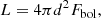
The Gaia mission (Gaia Collaboration 2016) and its data analysis provide astrometric measurements for each observed source in the sky. One of the parameters that is solved in the astrometric solution is the parallactic motion of the star due to its projected displacement on the sky with reference to the background stars. Gaia Data Release 2 (Gaia Collaboration 2018) provided the first measurements of parallax based on 22 months of data and derived a value of 3.44 ± 0.066 mas for HD 122563. Part of the analysis in C19 is based on this value. However Gaia continuously scans the sky and with more measurements over a longer baseline the parallax solution becomes more precise. Gaia Data Release 3 (Gaia Collaboration 2023b) released in June 2022 is based on 34 months of Gaia observations. The new parallax is 3.099 ± 0.033 mas, which is smaller than the previously published one, and therefore places the star further away, resulting in a higher intrinsic luminosity. Given this significant change in the parallax value, its luminosity needs to be revisited. To do this we use the Fbol values from C12 and S23, along with the latest parallax and the standard equation
 (1)
(1)
where d is the distance to the star. The parallax is the inverse of the distance, and because the relative error on the parallax is small, we do not use a prior to infer the distance (see e.g. Luri et al. 2018, for a discussion on this topic). We perform a very simple bootstrap method to derive the luminosity by perturbing the observational data for N = 10 000 simulations, and the resulting distributions give  and
and 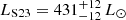 respectively.
We note that the Hipparcos mission was the first to record a parallax for HD 122563, equal to 4.22 ± 0.36 mas (van Leeuwen 2007), and this value was used in C12, when a first detailed comparison with stellar models was made. We also derive the radius and surface gravity of the star, where for the latter we assume that the star’s mass is centred on 0.80 M⊙ with an error of 0.05 M⊙, consistent with the star being a metal-poor, halo giant with an age on the order of ∼12.5 Gyr.
2.2.2. Luminosity from asteroseismology
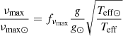
Asteroseismic analyses were performed on a data set of radial velocity measurements for HD 122563 observed with the SONG telescope (Andersen et al. 2014); songrefb, and in C19 a value of the asteroseismic quantity νmax (= 3.07 ± 0.05 μHz) was measured. This quantity is proportional to the surface gravity g of the star, and if we assume a mass, then we can derive its radius. As the angular diameter is known, we can then derive an asteroseismic distance independent of a distance measurement.
We follow here this same approach by using both the C12 and S23 Teff values along with the C19 νmax. We calculate g as :
 (2)
(2)
where fνmax = 1.0 and νmax, ⊙ = 3050 μHz (Kjeldsen & Bedding 1995). In this work we adopt Teff, ⊙ = 5772 K and log g⊙ = 4.438 dex from the IAU convention2 (Prša et al. 2016).
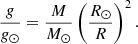
The equation for surface gravity is
 (3)
(3)
which can be rewritten as
 (4)
(4)
Here R⊙ = 6.957 × 1010 cm, while for M we again assume a distribution centred on 0.80 ± 0.05 M⊙. In this way R can then be derived, and finally the distance.
To estimate the stellar properties and uncertainties, we performed simulations and used their distributions to determine the asteroseismic luminosities and distances. These are given in the middle panel of Table 2; the star appears to be less luminous and closer than when using the parallax measurement.
Fundamental parameters of HD 122563 (Gaia DR3 3723554268436602240).
It is interesting to investigate also the impact of changing the assumption on the value of the stellar mass, and the value of νmax. If we assume a mass centred on 0.85 M⊙ instead of 0.80 M⊙, the effect is to increase the radius and thus the derived distance and luminosity at fixed νmax. A shift by +0.05 M⊙ increases the luminosity by ∼6% and the distance by ∼3%. Increasing the νmax value by 1σ will decrease the luminosity by 1.5% and the distance by < 1% at fixed mass.
There is additionally an empirical uncertainty on the value of fνmax in Eq. (2). It is under debate whether the classical scaling law for νmax should be modified to account for the chemical and structural differences in the outer layers of stellar targets compared to sun-like stars (we refer to Viani et al. 2017, and references therein). These corrections, however, change the derived luminosity and distance by smaller amounts when comparing to the effect of the offsets in mass and νmax described above. We therefore decided to be conservative and here we presently adopt the determination of the HD 122563 luminosity obtained via the classical (not accounting for second-order corrections) scaling law. Table 2 summarizes the various determinations of the fundamental parameters of this star.
2.3. Iron abundance and heavy elements distribution
The exact chemical composition of a stellar target is a critical ingredient when using this object as a benchmark for stellar models; this is because the effective temperature scale of stellar models – and this is particularly true in case of cool giant stars – critically depends on the iron content as well as α-element abundances. Iron is an important opacity source in the low-temperature regime (hence for the cool outer layers of giants), while α-elements, and in particular Mg, Si and O (in order of importance), due to their low energy ionization levels are fundamental electron donors and, hence have a huge impact on the H− ion opacity which is the major opacity contributor in the cool envelope of RGB stars (Cassisi & Salaris 2013).
Concerning the iron abundance [Fe/H] of HD 122563 there is a large spread of values in the literature. The estimates range from [Fe/H]= − 2.92 as provided by Afşar et al. (2016), to −2.75 from Karovicova et al. (2020), −2.7 from Collet et al. (2018), –2.64 from Jofré et al. (2014), ∼ − 2.5 as given by Prakapavičius et al. (2017), and [Fe/H]= − 2.43 (Amarsi et al. 2016). While part of this large spread of [Fe/H] values is due to the chosen reference solar composition adopted in the analyses, most of the variations are associated with the use of different methodologies and/or observational techniques.
A very accurate analysis of the chemical abundances for HD 122563 is the one by Amarsi et al. (2016), who made use of 3D non-LTE radiative transfer calculations based on the (3D) hydrodynamic STAGGER model atmospheres. They determined both LTE and non-LTE abundances from both FeI and FeII lines, and in this paper we adopt the stable abundance from the FeII lines, equal to [Fe/H]= − 2.43, as listed above. FeII lines are less affected by non-LTE effects and this estimate is therefore more reliable. However, we must keep in mind a conservative uncertainty of about 0.15 dex on this value.
Just as for [Fe/H], a large spread also exists concerning the α-element abundances. Significant differences in the literature stem from the adopted model atmospheres (1D versus 3D) and selected spectroscopic lines (we refer to Prakapavičius et al. 2017; Collet et al. 2018, for a discussion on this point). Collet et al. (2018) obtain [O/Fe] varying from +0.08 from molecular lines when compared to FeII, to +0.93 from the 630nm line when compared to FeI. They also derive [N/FeI] = +0.68 and [N/FeII] = +0.29. Prakapavičius et al. (2017) derive [O/Fe] = +0.07 to +0.37 using OH UV, IR, or the forbidden [OI] line. Jofré et al. (2015) derive [Mg/Fe] = + 0.29, [Si/Fe] = + 0.32 and [Ca/Fe] = +0.21, and Afşar et al. (2016) derive [Mg/Fe] = + 0.46, [Si/Fe] = + 0.45 and [Ca/Fe] = +0.38. A value of [Ca/Fe] = +0.33 is also given in Gaia DR3 based on the RVS spectra (Creevey et al. 2023; Recio-Blanco et al. 2023). In general, we find that the α/Fe corresponds to approximately +0.4 dex.
2.4. Photometric metallicity from a comparison to globular clusters
As an independent check of our adopted chemical composition, we have compared the position of HD 122563 in the (distance and reddening corrected) colour-magnitude diagram (CMD) with the RGBs of selected galactic globular clusters (GCs) with high-resolution spectroscopic determinations of their chemical composition. We employed NGC 6341 (M92), with [Fe/H]= − 2.30 (see, e.g. Lee 2023, and references therein), and NGC 6809 with an iron abundance equal to −2.01 (Rain et al. 2019). Both clusters have an α/Fe ≈ +0.40, similar to the α-enhancement of HD 122563.
To derive MG of HD 122563 we use the standard observational approach
 (5)
(5)
where G is the observed G magnitude from Gaia, ϖ is the parallax in mas, and AG is the extinction in G band. We employed the published AV = 0.01 ± 0.01 mag for the extinction and converted it to AG using the equations provided by Danielski et al. (2018) with the updated coefficients for DR3 given in the Gaia DR3 software webpages3. This equation requires as input the extinction defined at λ = 550 nm, called A0, and for this we used the value of AV. We employed the coefficients based on Teff and log g, using the adopted values described in the previous sections.
To derive the dereddened colour (GBP − GRP)0 = (GBP − GRP)−E(GBP − GRP), we applied the same method to estimate the extinction in the GBP and GRP bands – ABP and ARP – and then subtracted the colour excess E(GBP − GRP) from the observed (GBP − GRP). These quantities are summarised in Table 3.
Absolute magnitude and intrinsic colour for HD 122563.
As for the GCs, we used the Gaia data to select members and derive intrinsic magnitudes and colours for M92 and NGC 6809. We first selected all stars within a search radius around the centre of both clusters and calculated a distance in position dpos and proper motion dpm from the median values of the sample of stars, and then filtered the members based on a limit in both dpos and dpm. Once filtered on position and proper motion, we removed noisy sources or duplicated sources by filtering on
ipd_frac_multi_peak
ruwe, phot_bp_mean_flux_over_error
phot_rp_mean_flux_over_error
phot_g_mean_flux_over_error, phot_bp_n_obs
and phot_bp_n_blended_transits.
The actual limits imposed were based on inspection of the observed CMD to ensure that we retained sufficient members of the cluster in critical areas of their evolution stage, and removed as many outliers as possible. The details of the values used are given in Table 4. We note that to derive the distance we inspected the cluster members along the horizontal branch, by properly accounting for reddening at those Teff, and then adopted the distance needed to match the zero age horizontal branch (ZAHB) predicted by models with the clusters’ [Fe/H] value from the α-enhanced BaSTI library (Pietrinferni et al. 2021). This distance4 was then used for the calculation of MG of the member stars. It is worth noting that due to the vertical shape of the RGB – especially in the very metal-poor regime – a reasonable uncertainty of ∼0.10 − 0.15 mag in the GC distance moduli would not significantly affect the results of our comparison with HD 122563.
Properties and filtering of globular cluster members.
We have corrected the clusters’ photometry for extinction following the same procedure as for our star. For A0 we used the values of AV calculated from E(B − V) given by Harris (1996), using RV = 3.1. The extinctions were calculated for a reference Teff = 4600 K. As Table 4 implies, varying the Teff by ±100 K has a negligible impact on the adopted extinction.
The data for both globular clusters and HD 122563 are shown in Fig. 1. The position of HD 122563 in the CMD is consistent with the iron abundance estimated for M92, which overlaps with our adopted [Fe/H] by Amarsi et al. (2016) within the associated error bar.
We note that if the measured extinction towards M92 turned out to be underestimated, HD122563 would then appear more metal-rich. However, if the assumptions on the extinction towards NGC6809 were incorrect, the impact would be to simply increase or decrease the uncertainty on the photometric metallicity.
3. Stellar evolutionary tracks
The baseline stellar models adopted in this analysis are an updated version of the BaSTI stellar model library initially presented in Pietrinferni et al. (2004) and used by C19. The solar-scaled version of the updated models has been published in Hidalgo et al. (2018), and represents a significant improvement compared to the previous release of the database5 The changes in the input physics that affect the Teff scale of the RGB models are the following:
-
an updated solar heavy elements distribution provided by Caffau et al. (2011), which gives (Z/X)⊙ = 0.0209 and Z⊙ = 0.0153. Here X, Z are, as customary, the mass fractions of hydrogen and of all elements heavier than helium (metals), respectively. The previous BaSTI models employed the Grevesse & Noels (1993) solar metal mixture, which provided a larger value of Z⊙.
-
outer boundary conditions (BCs) obtained by integrating the atmospheric layers using the T(τ) relation by Vernazza et al. (1981), while the previous BaSTI models were based on the T(τ) by (Krishna Swamy 1966, herinafter K66). As discussed in Hidalgo et al. (2018), the alternative use of these atmospheric temperature stratifications (after the calibration of the mixing length αMLT), implies a difference in the Teff scale of metal-poor RGB models by about 60 K, the models based on the Vernazza et al. (1981)T(τ) relationship being cooler.
-
the efficiency of the superadiabatic convection has been fixed by using the same MLT formalism used in the earlier BaSTI release, but the value of αMLT has been recalibrated by computing an SSM (see the discussion in Hidalgo et al. 2018), to take into account the changes in the solar mixture and outer boundary conditions.
Given that we are dealing with a halo, metal-poor α-enhanced star, we employ here the new α-enhanced BaSTI models (Pietrinferni et al. 2021), which rely on the same physics inputs as the scaled-solar ones, but employ a heavy element distribution with all α-elements homogeneously enhanced by +0.4 dex with respect to Fe, compared to the solar-scaled distribution. In addition to the baseline stellar models available in the BaSTI library, we have used in our analysis additional dedicated sets of calculations, as discussed below.
4. Comparison between theory and observations
Figure 2 shows a comparison in the H-R diagram of our target star and the 0.80 M⊙ baseline RGB evolutionary tracks for [Fe/H]= − 2.43 (solid line, the same iron abundance adopted from the spectroscopic analysis by Amarsi et al. 2016), [Fe/H]= − 2.3 (long dashed line) and [Fe/H]= − 2.2 (short dashed line). At the luminosity derived from the Gaia parallax, the [Fe/H]= − 2.43 track is hotter by about ∼90 K and 130 K than the Teff determinations by S23 and C12, respectively. This means that – thanks mainly to the new Gaia DR3 parallax – the disagreement between theory and observations has been roughly halved in comparison with the analysis by Creevey et al. (2019).
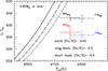 |
Fig. 2. H–R diagram of HD 122563. The different points with error bars correspond to the empirical measurements based on the two interferometric Teff estimates and the different methods for fixing the distance to the target (see Sect. 2.2 for more details). The various lines are the RGB evolutionary tracks of 0.8 M⊙α−enhanced stellar models with the labelled values of [Fe/H]. |
When considering the models for [Fe/H]= − 2.3 – the nominal [Fe/H] of M92 and roughly the upper limit to the adopted spectroscopic [Fe/H] – the discrepancy is reduced to about 70 K and 106 K compared to the S23 and C12 Teff estimates, respectively; in other words, at this (photometric-) metallicity the position of HD 122563 in the H-R diagram differs from the models at the level of about 2σ.
Given that in the explored metallicity regime, a change by 0.1 dex in the iron abundance changes the Teff scale of the RGB tracks by about ∼25 K, our baseline models would agree with observations at the 1σ level by increasing [Fe/H] by an additional 0.13 dex above [Fe/H]=−2.3 when adopting the S23 Teff, or by 0.3 dex in the case of the C12 Teff.
Figure 3 shows the same comparison of Fig. 2, but at fixed [Fe/H]= − 2.3 and for two different masses. It is evident that, for the selected iron abundance, the mass cannot be lower than about 0.78 M⊙, to have ages consistent with the cosmological age of ∼13.8 Gyr. Models for 0.78 M⊙ reduce the discrepancy between theory and observations at [Fe/H]= − 2.3 by only 10 K.
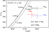 |
Fig. 3. As Fig. 2, but in this case the lines correspond to RGB evolutionary tracks for the labelled masses and [Fe/H]= − 2.3. Selected values of the model ages are shown along the tracks. |
4.1. Comparison with other stellar model libraries
In addition to our calculations, we have compared the position in the H–R diagram of HD 122563 with recent sets of evolutionary tracks from different groups. We have selected suitable 0.8 M⊙ evolutionary tracks from the PARSEC (Bressan et al. 2012), Dartmouth (Dotter et al. 2007), MIST (Choi et al. 2016), and the Victoria-Regina libraries (VandenBerg 2023).
While the BaSTI, Dartmouth and Victoria-Regina models are α-enhanced, the models from the other two libraries are based on a solar-scaled heavy element distribution, and in the comparison we chose tracks with a total metallicity [M/H] as close as possible to the metallicity derived from [Fe/H]= − 2.3 and [α/Fe]= + 0.4, and the solar metal distribution adopted in those calculations. This is an appropriate approximation, especially for metal-poor compositions, as first shown by Salaris et al. (1993).
In the case of the MIST models we used the online tool to calculate a 0.8 M⊙ track with the appropriate [M/H] ([M/H] = −1.99), while in the case of the PARSEC models we had to use the tracks with [M/H] closest to the appropriate value (namely [M/H] = −2.2 and −1.9, respectively). We compare all of these stellar tracks in Fig. 4.
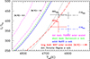 |
Fig. 4. As Fig. 2, but in this case, the lines correspond to the RGB 0.8 M⊙ evolutionary tracks from various stellar model libraries and different assumptions about the chemical composition (see labels and the text for more details). |
The Dartmouth and BaSTI tracks for [Fe/H]= − 2.3 are very similar, the BaSTI track being slightly cooler by just ∼5 K. The PARSEC tracks, even the one with a metallicity slightly higher than the appropriate value, are hotter than the BaSTI track, whilst the MIST and Victoria-Regina tracks are about 80 K cooler than BaSTI at the expected HD 122563’s brightness. Both Victoria and MIST tracks agree with the observations within less than 1σ when the S23 Teff is adopted, and the MIST track agrees with the data to less than 1σ also when the C12 Teff is used together with the Gaia-based luminosity.
Given this result, it is worthwhile to try and trace the origin of the difference of the Teff scale between the Victoria-Regina and MIST tracks and our BaSTI baseline one:
-
The first important difference is the approach used for fixing the BCs of the models. The MIST computations adopt BCs provided by model atmosphere computations (we refer to Choi et al. 2016, for more details); while the Victoria-Regina models rely on the integration of the solar T(τ) relation by Holweger & Mueller (1974);
-
Both MIST and Victoria-Regina models employ the solar heavy-element distribution by Asplund et al. (2009), which is different from that adopted in the other selected libraries. PARSEC and BaSTI are based on the Caffau et al. (2011) solar metal mixture, while the Dartmouth library adopts the solar heavy element distribution by Grevesse & Sauval (1998). The different metal mixture affects directly the radiative opacities, and indirectly the mixing length calibration. In fact the lower solar metallicity induced by the Asplund et al. (2009) metal distribution compared to Caffau et al. (2011) and Grevesse & Sauval (1998) requires a smaller value of the mixing length to calibrate the solar model and this, in turn, implies a lower Teff of the RGB models.
In the following, we discuss these two points in more detail.
4.2. The role of outer boundary conditions
The Teff scale of RGB models is significantly dependent on the approach used for fixing the BCs required to solve the set of stellar structure equations (see, e.g., Salaris et al. 2002; VandenBerg et al. 2008; Salaris & Cassisi 2015; Choi et al. 2018, and references therein). Although, once the mixing length parameter is re-calibrated by means of an SSM, the impact of using different BCs on the RGB Teff scale is reduced. Significant differences do exist among RGB stellar models based on different choices for the calculation of the atmospheric thermal stratification and the BCs. As shown by Salaris et al. (2002), and more recently by Choi et al. (2018), the use of different BCs can lead to offsets by ±100 K on the RGB, even if the mixing length αMLT has been properly calibrated to the solar value in the models.
We have therefore tested different choices for the BCs in the metal-poor regime of our target. To do this, we have computed 0.8 M⊙ evolutionary tracks for [Fe/H]= − 2.3 by using the same input physics as our baseline BaSTI models, but relying on the integration of different T(τ) relationships for the atmospheric layers. We used the KS66 T(τ), the Eddington (grey) atmosphere, and the Holweger & Mueller (1974) relationship (hereinafter HM74). In each case we have fixed the mixing length parameter by calibrating a SSM, and we obtained αMLT = 1.799 with the KS66 T(τ), αMLT = 2.109 with the HM74 one, and 2.214 for the grey atmosphere. For comparison, in our baseline models we use αMLT = 2.006 with the Vernazza et al. (1981)T(τ).
Figure 5 shows the results of these calculations, which extends the analysis performed in Hidalgo et al. (2018) to the very metal-poor regime. The RGBs calculated with the grey Eddington T(τ) are very close to our baseline calculations, but with a slightly different slope. The RGB computed with the KS66 T(τ) is hotter than the baseline model by about 30 K, a smaller difference (but in the same direction) than the case at higher metallicity, while the RGB calculated with the HM74 T(τ) is cooler than the reference one by ∼40 K. This is different than the case at solar metallicity where RGBs with the HM74 T(τ) are about 40 K hotter than calculations with the Vernazza et al. (1981)T(τ).
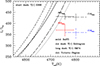 |
Fig. 5. As Fig. 6 but for various assumptions about the thermal stratification adopted in the atmospheric stellar layers (see labels) in the Basti models. The evolutionary track for the 0.8 M⊙ model as provided by the Victoria-Regina library is also shown for comparison. |
Figure 5 shows that the RGB calculated with the HM74 T(τ) is very close to the RGB of the Victoria-Regina models, showing differences of less than 20 K at the luminosity of our target star. This also implies that the impact of the different solar metal mixture is minor, and if we use the results of the next section about the variation of the RGB Teff induced by a given variation of αMLT, we find that the remaining temperature difference is due to the different solar calibrated αMLT in the Victoria-Regina models –smaller by 0.1 than our calibration with the HM74 T(τ)– induced by the different choice of the solar metal mixture. Based on these results, we can predict that the use of the solar heavy-element distribution recently suggested by Magg et al. (2022) – which provides a very similar but slightly larger solar metallicity than that by Caffau et al. (2011) – would not have any significant impact on our analysis.
It seems therefore that one way to reduce or erase the discrepancy between our baseline BaSTI models and the observations of this star is basically to employ a different T(τ) relation to calculate the BCs. It is however worth recalling that Salaris & Cassisi (2015) have shown that RGB models calculated with the Vernazza et al. (1981)T(τ) relation and a solar calibrated mixing length seem adequate to reproduce the effective temperature of RGB stars with α/Fe = 0.0 in the metal-rich regime.
Based on these tests, the interpretation of the results with the MIST model is less clear. As extensively discussed by Choi et al. (2018), the thermal stratification provided by the model atmospheres used in Choi et al. (2016) is well reproduced by the Vernazza et al. (1981)T(τ). But it is then hard to understand the offset and the different slope of the RGB compared to the BaSTI models that use the Vernazza et al. (1981)T(τ), given also the small impact of the different solar metallicity, as deduced by the comparison with the Victoria-Regina models.
4.3. The value of αMLT
An alternative possibility to explain the disagreement between the Teff of the BaSTI (but also Dartmouth and PARSEC) RGBs and the target star, assuming that their choices to fix the BCs and possibly the solar metal mixture are the ‘correct’ ones, is a variation of αMLT compared to the solar calibrated value. There is abundant literature on this subject, and the reader can refer to the recent review by Joyce & Tayar (2023).
In a recent work based on APOKASC data, Salaris et al. (2018) found that for stars with solar-scaled heavy element composition in the [Fe/H] range between ∼0.4 and ∼−0.6, there is a good agreement between theoretical and observed Teff with models consistent with the baseline BaSTI calculations, calculated with solar calibrated αMLT. However, the same models appeared to be too hot when compared to stars with α-enhanced composition in the range −0.7 < [Fe/H]< − 0.35 dex. This result is qualitatively consistent with what we find in the comparison of our baseline BaSTI models with HD 122563.
To determine what variation of αMLT is required to bring the baseline BaSTI models in better agreement with the observations of HD 122563, we have calculated additional 0.8 M⊙α-enhanced tracks with [Fe/H]= − 2.3 and mixing length reduced from the solar value αMLT, ⊙ by two different amounts, as shown in Fig. 6.
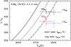 |
Fig. 6. Same as Fig. 2 but for 0.8 M⊙ evolutionary tracks, computed by reducing the calibrated solar αMLT, ⊙ = 2.006 by various amounts (see labels). |
We find that at this metallicity and in the relevant range of luminosities, a reduction of αMLT by 0.1 decreases the model Teff by ∼+45 K. Hence, a decrease of αMLT by 0.1 − 0.2 is in principle able to put the BaSTI models in agreement with the observations, for a target metallicity [Fe/H] = −2.3.
A similar result, that is the need for a sub-solar αMLT to better reproduce the Teff of metal-poor stars, has been found by Joyce & Chaboyer (2018) for a sample of main sequence and sub-giant stars by using their own evolutionary code. This has also been suggested by C12, C19 and Creevey et al. (2015).
5. Conclusions
From the previous analysis, it appears clear that if [Fe/H] ∼ − 2.3 for HD 122563 (compatible with the metallicity of M92), both Victoria-Regina and MIST models are able – within the estimated uncertainties on luminosity and Teff – to match the star’s position in the H–R diagram. If its iron content is equal to ∼ − 2.4 dex or lower, there are no current sets of stellar models able to match its luminosity and Teff.
A possibility to improve the agreement of BaSTI (as well as Dartmouth and PARSEC) models with the star in the H–R diagram is to use different BCs in the model calculations, or change the mixing length while keeping the choice of the BCs fixed. For instance either the use of the HM74 atmospheric thermal stratification to calculate the BCs, or a significant reduction of the mixing length by about 0.2 with respect to the solar calibrated value, could reconcile the models with the position of the star in the H–R diagram, within the errors.
Observationally, a more stringent test of the metal poor RGB models’ Teff scale requires not only a more robust assessment of the observational properties of HD 122563 via a more accurate astrometric, spectroscopic and interferometric studies, but also a larger sample of metal-poor stars with accurate empirical determinations of their luminosities, Teff, chemical composition and – if possible – mass, using asteroseismology in the case of single stars, or dynamical measurements in the case of binary systems.
From a theoretical point of view, it is crucial to minimise the uncertainties in the calculation of the superadiabatic temperature gradients in the convective envelopes of RGB models, and the calculation of the outer boundary conditions. The current generation of 3D radiation-hydrodynamics simulations of stellar convective envelopes (e.g., Magic et al. 2013; Trampedach et al. 2014b,a; Magic et al. 2015) reach the metallicity regime of HD 122563 (Magic et al. 2013), but do not cover surface gravities low enough to be employed to help model stars like HD 122563. An extension of this type of simulations to lower surface gravities is much needed.
Additional free parameters are embedded in the MLT formalism, but they are generally fixed a priori, giving origin to different ‘flavours’ of the MLT (see, e.g., Salaris & Cassisi 2008, and references therein). Different MLT flavours provide essentially the same evolutionary tracks once the parameter αMLT is accordingly calibrated on the Sun via the SSM.
https://www.iau.org/static/resolutions/IAU2015_English.pdf Resolution B3.
We note that the estimated distance for the two GCs are in fair agreement with the estimates provided by VandenBerg (2023) by using the same approach but his own ZAHB models and different photometric data: ∼8520 pc and ∼5200 pc for M92 and NGC 6809, respectively.
Unlike previous BaSTI models, the new ones include also atomic diffusion. However, atomic diffusion does not have any significant impact on the Teff of RGB models, because the 1st dredge-up basically restores the initial metallicity in the RGB envelopes (see, e.g., Cassisi & Salaris 2013, for a more detailed discussion on this topic).
Acknowledgments
SC has been funded by the European Union – NextGenerationEU” RRF M4C2 1.1 n: 2022HY2NSX. “CHRONOS: adjusting the clock(s) to unveil the CHRONO-chemo-dynamical Structure of the Galaxy” (PI: S. Cassisi), and INAF 2023 Theory grant “Lasting” (PI: S. Cassisi). SC also warmly acknowledges the kind hospitality at the Université de la Côte d’Azur, Nice, where a large part of this investigation has been performed. MS acknowledges support from The Science and Technology Facilities Council Consolidated Grant ST/V00087X/1. The authors acknowledge the financial support from the scientific council of the Observatoire de la Côte d’Azur under its strategic scientific program. SC warmly thanks D. Vandenberg for providing his stellar evolution models as well as for several interesting discussions. This work has made use of data from the European Space Agency (ESA) mission Gaia (https://www.cosmos.esa.int/gaia), processed by the Gaia Data Processing and Analysis Consortium (DPAC, https://www.cosmos.esa.int/web/gaia/dpac/consortium). Funding for the DPAC has been provided by national institutions, in particular the institutions participating in the Gaia Multilateral Agreement.
References
- Afşar, M., Sneden, C., Frebel, A., et al. 2016, ApJ, 819, 103 [Google Scholar]
- Amarsi, A. M., Lind, K., Asplund, M., Barklem, P. S., & Collet, R. 2016, MNRAS, 463, 1518 [NASA ADS] [CrossRef] [Google Scholar]
- Andersen, M. F., Grundahl, F., Christensen-Dalsgaard, J., et al. 2014, Rev. Mex. Astron. Astrofis. Conf. Ser., 45, 83 [NASA ADS] [Google Scholar]
- Asplund, M., Grevesse, N., Sauval, A. J., & Scott, P. 2009, ARA&A, 47, 481 [NASA ADS] [CrossRef] [Google Scholar]
- Berezhiani, Z., Ciarcelluti, P., Cassisi, S., & Pietrinferni, A. 2006, Astropart. Phys., 24, 495 [NASA ADS] [CrossRef] [Google Scholar]
- Böhm-Vitense, E. 1958, ZAp, 46, 108 [NASA ADS] [Google Scholar]
- Borucki, W. J., Koch, D., Basri, G., et al. 2010, Science, 327, 977 [Google Scholar]
- Bressan, A., Marigo, P., Girardi, L., et al. 2012, MNRAS, 427, 127 [NASA ADS] [CrossRef] [Google Scholar]
- Caffau, E., Ludwig, H.-G., Steffen, M., Freytag, B., & Bonifacio, P. 2011, Sol. Phys., 268, 255 [Google Scholar]
- Casagrande, L., Portinari, L., Glass, I. S., et al. 2014, MNRAS, 439, 2060 [Google Scholar]
- Cassisi, S., & Salaris, M. 2013, Old Stellar Populations: How to Study the Fossil Record of Galaxy Formation (Wiley-VCH) [CrossRef] [Google Scholar]
- Cassisi, S., Castellani, V., Degl’Innocenti, S., Fiorentini, G., & Ricci, B. 2000, Phys. Lett. B, 481, 323 [CrossRef] [Google Scholar]
- Castellani, V., & deglInnocenti, S. 1993, ApJ, 402, 574 [NASA ADS] [CrossRef] [Google Scholar]
- Chaplin, W. J., Serenelli, A. M., Miglio, A., et al. 2020, Nat. Astron., 4, 382 [Google Scholar]
- Choi, J., Dotter, A., Conroy, C., et al. 2016, ApJ, 823, 102 [Google Scholar]
- Choi, J., Dotter, A., Conroy, C., & Ting, Y.-S. 2018, ApJ, 860, 131 [NASA ADS] [CrossRef] [Google Scholar]
- Collet, R., Nordlund, Å., Asplund, M., Hayek, W., & Trampedach, R. 2018, MNRAS, 475, 3369 [NASA ADS] [CrossRef] [Google Scholar]
- Creevey, O. L., Thévenin, F., Boyajian, T. S., et al. 2012, A&A, 545, A17 [NASA ADS] [CrossRef] [EDP Sciences] [Google Scholar]
- Creevey, O. L., Thévenin, F., Berio, P., et al. 2015, A&A, 575, A26 [NASA ADS] [CrossRef] [EDP Sciences] [Google Scholar]
- Creevey, O., Grundahl, F., Thévenin, F., et al. 2019, A&A, 625, A33 [NASA ADS] [CrossRef] [EDP Sciences] [Google Scholar]
- Creevey, O. L., Sordo, R., Pailler, F., et al. 2023, A&A, 674, A26 [NASA ADS] [CrossRef] [EDP Sciences] [Google Scholar]
- Danielski, C., Babusiaux, C., Ruiz-Dern, L., Sartoretti, P., & Arenou, F. 2018, A&A, 614, A19 [NASA ADS] [CrossRef] [EDP Sciences] [Google Scholar]
- De Ridder, J., Molenberghs, G., Eyer, L., & Aerts, C. 2016, A&A, 595, L3 [NASA ADS] [CrossRef] [EDP Sciences] [Google Scholar]
- Dotter, A., Chaboyer, B., Jevremović, D., et al. 2007, AJ, 134, 376 [NASA ADS] [CrossRef] [Google Scholar]
- Gaia Collaboration (Prusti, T., et al.) 2016, A&A, 595, A1 [NASA ADS] [CrossRef] [EDP Sciences] [Google Scholar]
- Gaia Collaboration (Brown, A. G. A., et al.) 2018, A&A, 616, A1 [NASA ADS] [CrossRef] [EDP Sciences] [Google Scholar]
- Gaia Collaboration (Montegriffo, P., et al.) 2023a, A&A, 674, A33 [CrossRef] [EDP Sciences] [Google Scholar]
- Gaia Collaboration (Vallenari, A., et al.) 2023b, A&A, 674, A1 [NASA ADS] [CrossRef] [EDP Sciences] [Google Scholar]
- García, R. A., Hekker, S., Stello, D., et al. 2011, MNRAS, 414, L6 [NASA ADS] [CrossRef] [Google Scholar]
- Gilmore, G., Randich, S., Asplund, M., et al. 2012, The Messenger, 147, 25 [NASA ADS] [Google Scholar]
- Grevesse, N., & Noels, A. 1993, Phys. Scr. Vol. T, 47, 133 [NASA ADS] [CrossRef] [Google Scholar]
- Grevesse, N., & Sauval, A. J. 1998, Space Sci. Rev., 85, 161 [Google Scholar]
- Grundahl, F., Fredslund Andersen, M., Christensen-Dalsgaard, J., et al. 2017, ApJ, 836, 142 [Google Scholar]
- Harris, W. E. 1996, AJ, 112, 1487 [Google Scholar]
- Hidalgo, S. L., Pietrinferni, A., Cassisi, S., et al. 2018, ApJ, 856, 125 [Google Scholar]
- Holweger, H., & Mueller, E. A. 1974, Sol. Phys., 39, 19 [NASA ADS] [CrossRef] [Google Scholar]
- Jofré, P., Heiter, U., Soubiran, C., et al. 2014, A&A, 564, A133 [NASA ADS] [CrossRef] [EDP Sciences] [Google Scholar]
- Jofré, P., Heiter, U., Soubiran, C., et al. 2015, A&A, 582, A81 [Google Scholar]
- Jofré, P., Heiter, U., Worley, C. C., et al. 2017, A&A, 601, A38 [Google Scholar]
- Joyce, M., & Chaboyer, B. 2018, ApJ, 856, 10 [Google Scholar]
- Joyce, M., & Tayar, J. 2023, Galaxies, 11, 75 [NASA ADS] [CrossRef] [Google Scholar]
- Karovicova, I., White, T. R., Nordlander, T., et al. 2018, MNRAS, 475, L81 [Google Scholar]
- Karovicova, I., White, T. R., Nordlander, T., et al. 2020, A&A, 640, A25 [NASA ADS] [CrossRef] [EDP Sciences] [Google Scholar]
- Kjeldsen, H., & Bedding, T. R. 1995, A&A, 293, 87 [NASA ADS] [Google Scholar]
- Krishna Swamy, K. S. 1966, ApJ, 145, 174 [Google Scholar]
- Kuszlewicz, J. S., Hon, M., & Huber, D. 2023, ApJ, 954, 152 [NASA ADS] [CrossRef] [Google Scholar]
- Lee, J.-W. 2023, ApJ, 948, L16 [NASA ADS] [CrossRef] [Google Scholar]
- Luri, X., Brown, A. G. A., Sarro, L. M., et al. 2018, A&A, 616, A9 [NASA ADS] [CrossRef] [EDP Sciences] [Google Scholar]
- Magg, E., Bergemann, M., Serenelli, A., et al. 2022, A&A, 661, A140 [NASA ADS] [CrossRef] [EDP Sciences] [Google Scholar]
- Magic, Z., Collet, R., Asplund, M., et al. 2013, A&A, 557, A26 [NASA ADS] [CrossRef] [EDP Sciences] [Google Scholar]
- Magic, Z., Weiss, A., & Asplund, M. 2015, A&A, 573, A89 [NASA ADS] [CrossRef] [EDP Sciences] [Google Scholar]
- Mathur, S., García, R. A., Huber, D., et al. 2016, ApJ, 827, 50 [NASA ADS] [CrossRef] [Google Scholar]
- Mathur, S., García, R. A., Breton, S., et al. 2022, A&A, 657, A31 [NASA ADS] [CrossRef] [EDP Sciences] [Google Scholar]
- Miglio, A., Chaplin, W. J., Brogaard, K., et al. 2016, MNRAS, 461, 760 [NASA ADS] [CrossRef] [Google Scholar]
- Miglio, A., Chiappini, C., Mackereth, J. T., et al. 2021, A&A, 645, A85 [NASA ADS] [CrossRef] [EDP Sciences] [Google Scholar]
- Pietrinferni, A., Cassisi, S., Salaris, M., & Castelli, F. 2004, ApJ, 612, 168 [Google Scholar]
- Pietrinferni, A., Hidalgo, S., Cassisi, S., et al. 2021, ApJ, 908, 102 [NASA ADS] [CrossRef] [Google Scholar]
- Prakapavičius, D., Kučinskas, A., Dobrovolskas, V., et al. 2017, A&A, 599, A128 [NASA ADS] [CrossRef] [EDP Sciences] [Google Scholar]
- Prša, A., Harmanec, P., Torres, G., et al. 2016, AJ, 152, 41 [Google Scholar]
- Rain, M. J., Villanova, S., Munõz, C., & Valenzuela-Calderon, C. 2019, MNRAS, 483, 1674 [NASA ADS] [CrossRef] [Google Scholar]
- Recio-Blanco, A., de Laverny, P., Palicio, P. A., et al. 2023, A&A, 674, A29 [NASA ADS] [CrossRef] [EDP Sciences] [Google Scholar]
- Salaris, M., & Cassisi, S. 1996, A&A, 305, 858 [NASA ADS] [Google Scholar]
- Salaris, M., & Cassisi, S. 2008, A&A, 487, 1075 [NASA ADS] [CrossRef] [EDP Sciences] [Google Scholar]
- Salaris, M., & Cassisi, S. 2015, A&A, 577, A60 [CrossRef] [EDP Sciences] [Google Scholar]
- Salaris, M., Chieffi, A., & Straniero, O. 1993, ApJ, 414, 580 [NASA ADS] [CrossRef] [Google Scholar]
- Salaris, M., Cassisi, S., & Weiss, A. 2002, PASP, 114, 375 [NASA ADS] [CrossRef] [Google Scholar]
- Salaris, M., Cassisi, S., Schiavon, R. P., & Pietrinferni, A. 2018, A&A, 612, A68 [NASA ADS] [CrossRef] [EDP Sciences] [Google Scholar]
- Serenelli, A., Weiss, A., Cassisi, S., Salaris, M., & Pietrinferni, A. 2017, A&A, 606, A33 [NASA ADS] [CrossRef] [EDP Sciences] [Google Scholar]
- Silva Aguirre, V., Bojsen-Hansen, M., Slumstrup, D., et al. 2018, MNRAS, 475, 5487 [NASA ADS] [Google Scholar]
- Soubiran, C., Creevey, O. L., Lagarde, N., et al. 2024, A&A, 682, A145 [NASA ADS] [CrossRef] [EDP Sciences] [Google Scholar]
- Tayar, J., Somers, G., Pinsonneault, M. H., et al. 2017, ApJ, 840, 17 [NASA ADS] [CrossRef] [Google Scholar]
- Trampedach, R., Stein, R. F., Christensen-Dalsgaard, J., Nordlund, Å., & Asplund, M. 2014a, MNRAS, 442, 805 [NASA ADS] [CrossRef] [Google Scholar]
- Trampedach, R., Stein, R. F., Christensen-Dalsgaard, J., Nordlund, Å., & Asplund, M. 2014b, MNRAS, 445, 4366 [NASA ADS] [CrossRef] [Google Scholar]
- van Leeuwen, F. 2007, A&A, 474, 653 [CrossRef] [EDP Sciences] [Google Scholar]
- VandenBerg, D. A. 2023, MNRAS, 518, 4517 [Google Scholar]
- VandenBerg, D. A., Edvardsson, B., Eriksson, K., & Gustafsson, B. 2008, ApJ, 675, 746 [NASA ADS] [CrossRef] [Google Scholar]
- Vernazza, J. E., Avrett, E. H., & Loeser, R. 1981, ApJS, 45, 635 [Google Scholar]
- Viani, L. S., Basu, S., Chaplin, W. J., Davies, G. R., & Elsworth, Y. 2017, ApJ, 843, 11 [NASA ADS] [CrossRef] [Google Scholar]
- Vrard, M., Cunha, M. S., Bossini, D., et al. 2022, Nat. Commun., 13, 7553 [CrossRef] [Google Scholar]
- Zoccali, M., Renzini, A., Ortolani, S., et al. 2003, A&A, 399, 931 [NASA ADS] [CrossRef] [EDP Sciences] [Google Scholar]
All Tables
All Figures
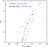 |
Fig. 1. MG − (GBP − GRP)0 CMD of M92, NGC 6809, and HD 122563 (see Sect. 2 for more details). |
| In the text | |
|
Fig. 2. H–R diagram of HD 122563. The different points with error bars correspond to the empirical measurements based on the two interferometric Teff estimates and the different methods for fixing the distance to the target (see Sect. 2.2 for more details). The various lines are the RGB evolutionary tracks of 0.8 M⊙α−enhanced stellar models with the labelled values of [Fe/H]. |
| In the text | |
|
Fig. 3. As Fig. 2, but in this case the lines correspond to RGB evolutionary tracks for the labelled masses and [Fe/H]= − 2.3. Selected values of the model ages are shown along the tracks. |
| In the text | |
|
Fig. 4. As Fig. 2, but in this case, the lines correspond to the RGB 0.8 M⊙ evolutionary tracks from various stellar model libraries and different assumptions about the chemical composition (see labels and the text for more details). |
| In the text | |
|
Fig. 5. As Fig. 6 but for various assumptions about the thermal stratification adopted in the atmospheric stellar layers (see labels) in the Basti models. The evolutionary track for the 0.8 M⊙ model as provided by the Victoria-Regina library is also shown for comparison. |
| In the text | |
|
Fig. 6. Same as Fig. 2 but for 0.8 M⊙ evolutionary tracks, computed by reducing the calibrated solar αMLT, ⊙ = 2.006 by various amounts (see labels). |
| In the text | |
Current usage metrics show cumulative count of Article Views (full-text article views including HTML views, PDF and ePub downloads, according to the available data) and Abstracts Views on Vision4Press platform.
Data correspond to usage on the plateform after 2015. The current usage metrics is available 48-96 hours after online publication and is updated daily on week days.
Initial download of the metrics may take a while.