| Issue |
A&A
Volume 689, September 2024
|
|
|---|---|---|
| Article Number | A235 | |
| Number of page(s) | 21 | |
| Section | Planets and planetary systems | |
| DOI | https://doi.org/10.1051/0004-6361/202449456 | |
| Published online | 16 September 2024 | |
The GAPS Programme at TNG
LVIII. Two multi-planet systems with long-period substellar companions around metal-rich stars★
1
Department of Physics and Astronomy, University of Padova,
Vicolo dell’Osservatorio 2,
35122
Padova,
Italy
2
INAF, Astrophysical Observatory of Padova,
Vicolo dell’Osservatorio 5,
35122
Padova,
Italy
3
INAF, Astrophysical Observatory of Turin,
Via Osservatorio 20,
10025
Pino Torinese (TO),
Italy
4
Department of Physics and Astronomy, University of Padova,
Via Marzolo 8,
35131
Padova,
Italy
5
INAF, Astronomical Observatory of Rome,
Via Frascati 33,
00178
Monte Porzio Catone (RM),
Italy
6
Department of Physics, University of Rome Tor Vergata,
Via della Ricerca Scientifica 1,
00133
Rome,
Italy
7
INAF, Astronomical Observatory of Palermo,
Piazza del Parlamento 1,
90134
Palermo,
Italy
8
INAF, Astronomical Observatory of Trieste,
Via Tiepolo 11,
34143
Trieste,
Italy
9
Laboratoire J. L. Lagrange, Université Côte d’Azur, CNRS,
Observatoire de la Côte d’Azur,
06304
Nice,
France
10
Department d’astronomie de l’Université de Genève,
Chemin Pegasi 51,
1290
Versoix,
Switzerland
11
Department of Physics, University of Rome “Tor Vergata”,
Via della Ricerca Scientifica 1,
00133
Rome,
Italy
12
INAF, Osservatorio Astrofisico di Catania,
Via S. Sofia 78,
95123
Catania,
Italy
13
Aix Marseille Univ., CNRS, CNES, LAM,
Marseille,
France
Received:
2
February
2024
Accepted:
26
July
2024
Context. Due to observational biases, a large fraction of known exoplanets are short-period objects. However, the search for planets began more than 20 yr ago, and so it is already possible – with the use of a suitable dataset – to begin exploring a wider range of the parameter space, such as that encompassing long-period planets.
Aims. The aim of this paper is to investigate the presence of long-period giant companions in two systems where one or more planets are already known and for which a long-term trend in the radial velocities (RVs) was noted in previous works.
Methods. Over the last 11 yr, we have collected 122 spectra of HD 75898 and 72 spectra of HD 11506 with the High Accuracy Radial velocity Planet Searcher for the Northern hemisphere (HARPS-N) in the framework of the Global Architecture of Planetary Systems (GAPS) project, from which we derived precise RV and activity indicator measurements. Additional RV data from the High-Resolution Echelle Spectrometer (HIRES) are also used here to increase the total time span. For our RV analysis, we used PyORBIT, an advanced Python tool for the simultaneous Bayesian analysis of RVs and stellar activity indicators. In addition, we used astrometric (Gaia DR3) and imaging archive data to complete our analysis. In particular, we combined RVs and astrometry to better constrain the mass and period of the new long-period companions.
Results. We find evidence for one additional long-period companion (gas giant planet or brown dwarf) in both systems considered. The new candidate for HD 75898 has a period of roughly 18 yr and a true mass of around 8.5 Mj. For HD 11506, we confirm the new object (planet d) recently announced using HIRES data but we find that the period and true mass are both almost double the values based on HIRES results (Pd ~ 72 yr, Md ~ 13 Mj). In addition, for HD 75898, we also find evidence of an activity cycle affecting RVs with a period of one order of magnitude lower than found in the literature.
Key words: techniques: radial velocities / planets and satellites: detection / stars: individual: HD 75898 / stars: individual: HD 11506 / stars: solar-type
© The Authors 2024
 Open Access article, published by EDP Sciences, under the terms of the Creative Commons Attribution License (https://creativecommons.org/licenses/by/4.0), which permits unrestricted use, distribution, and reproduction in any medium, provided the original work is properly cited.
This article is published in open access under the Subscribe to Open model. Subscribe to A&A to support open access publication.
1 Introduction
Since the discovery of the first exoplanet in the 1990s, many similar discoveries have been made, revealing a broad diversity in planetary system architectures. In particular, it seems that the architecture of our Solar System is not common at all, while there are classes of planets that are absent in the Solar System but are present around other stars, such as super-Earths and hot Jupiters. As more and more planets are discovered, it becomes possible to perform statistical analyses of the properties and demographics of these systems (e.g., Mayor et al. 2011, Barbato et al. 2018, and Pinamonti et al. 2022). Unfortunately, the two most common methods used to discover exoplanets – transits and radial velocities – suffer from strong observational biases that make it harder to find objects at long orbital periods. In addition, several sources of uncertainty complicate the situation, such as stellar activity (Santos et al. 2010; Dumusque et al. 2011; Lovis et al. 2011, and Carolo et al. 2014). Nevertheless, we can now find objects at even larger separations from their star, and indeed there are currently a few hundred planets known with P > 1000 days. This is possible thanks to a combination of different factors. From the instrumental point of view, there are now telescopes able to probe the sub-m s−1 regime and/or operate for decades: the High-Resolution Echelle Spectrometer (HIRES), the High Accuracy Radial velocity Planet Searcher (HARPS), its twin for the Northern hemisphere (HARPS-N), and the Echelle SPectrograph for Rocky Exoplanet and Stable Spectroscopic Observations (ESPRESSO), and this is important because the RV signal of long-period planets is lower compared to that of planets with the same mass but a shorter period. We have also developed advanced computational techniques, such as the Gaussian process (GP), which can handle stellar activity and take into account its contribution to the RV signal (e.g., Grunblatt et al. 2015; López-Morales et al. 2016; Perger et al. 2021; Mantovan et al. 2024). The best way to find giant planets with orbital periods similar to those of the Solar System is to perform long-term RV campaigns. As this was the first technique used to observe exoplanets, we have more than 20 years of data for certain stars, which – if properly combined – can reveal the presence of planetary signals with orbital periods lasting a few decades. Furthermore, direct imaging and astrom-etry provide deeper insights into planetary populations, because both are more sensitive to planets that are very far from their stars. Unfortunately, these are in turn biased towards more massive objects, although future instruments will hopefully display a greater sensitivity.
In 2012, the GAPS (Global Architecture of Planetary Sys-tems1) project was started, with the aim being to obtain a more complete comprehension of planetary bodies and their systems (e.g., Sozzetti et al. 2013 and Covino et al. 2013). The GAPS team includes a large fraction of the Italian astronomical community working in this field and has obtained great results in the last decade thanks to the awarded observing time at the Italian telescope TNG (La Palma, Canary Islands) with HARPS-N (Cosentino et al. 2012). For this paper, we consider the data obtained since the beginning of the GAPS project as part of the Known Planets (KP) sub-program. Our aim here is to search for additional companions in planetary systems where at least one object is already known in order to widen our knowledge of multiplanet systems. Some results from this project have already been published (e.g., Benatti et al. 2020). The original KP target list includes 16 objects, and in this work we investigate two of them: HD 75898 and HD 11506.
Section 2 describes our observations and the archive data. In Sect. 3, we describe our analysis of the target stars and our derivation of their physical and spectroscopic parameters. In Sect. 4, we outline the data-analysis tools that we used. In Sects. 5 and 6 we present the results for HD 75898 and HD 11506, respectively. Section 7 contains a discussion about the implications of our results. In Sect. 8 we summarize our conclusions.
2 Observations and data analysis
2.1 High-resolution spectroscopy
2.1.1 HARPS-N spectra
In the framework of the GAPS program, we have been observing our targets since 2012 with the HARPS-N spectrograph at TNG, with a typical integration time of 900 s for both stars. For HD 75898, we collected 122 spectra from November 13, 2012, to April 8, 2023. For HD 11506, we gathered 72 spectra between August 23, 2013, and November 25, 2022. For both stars, Radial Velocities (RVs) were obtained with the HARPS-N pipeline using the online tool YABI2 (Hunter et al. 2015), deployed at IA2 Data Centre, using a G2 mask for the cross-correlation function (CCF). We also exploited the YABI tool, with the procedure based on Lovis et al. (2011), to measure the S Index, calibrated onto the Mount Wilson scale, and the chromo-spheric activity index log R′HK. Six spectra of HD 75898, taken before October2012, with only one of the two CCDs sensor oper-ational (Desidera et al. 2013) were removed from the analysis, considering the additional free offset parameter, their larger RV errors, and lack of S -index measurements. The full HARPS-N RV time series is available at the CDS.
2.1.2 Archive and literature data
We used publicly available data taken with HIRES at Keck (Butler et al. 2017). These include 93 data points (RVs and SMW) for HD 75898 and 114 data points for HD 11506. The authors state that their S-index values are already calibrated to the Mount Wilson scale, and are therefore, in principle, homogeneously calibrated to the HARPS-N data; however, they do not provide errorbars for this quantity. Therefore, for each target, we took bunches of data points with very high temporal sampling (~ 1/day) and calculated their standard deviations. After doing so for as many clusters of points as possible, we made the average of all the sigmas and used the resulting value as the error bar for the whole set. We admit that the errors obtained in this way could be overestimated if there is a short-term scatter (e.g., stellar rotation) or underestimated if there is a long-term instrumental error. In any case, we introduced a jitter term in our analysis to account for additional sources of errors. The authors also describe the CCD upgrade that took place in August 2004, which significantly improved the quality of the measurements, and they did not find any significant offset between data taken before and after such an operation. Nevertheless, we decided to treat these as two different data sets (different offset and jitter terms) as a conservative approach for HD 11506. For HD 75898, since only 4 data points were taken before that date, we decided to use the same offset term for the whole HIRES time series.
We also acknowledge that there are some data taken with the instruments SOPHIE (Spectrographe pour l’Observation des Phénomènes des Intérieurs stellaires et des Exoplanètes) and ELODIE for HD 75898. However, we found that their addition does not bring significant improvements to our results. The ELODIE set includes 22 points, but their error bars range from 10 to 40 m s−1, so one order of magnitude greater than the other instruments. On the other hand, the SOPHIE set has an average error bar of around 2.7 m s−1 but there are only 5 points that do not extend the temporal baseline. The final data sets for each target are shown in Table 1, together with the total time span of the observations.
2.2 High-contrast imaging and relative astrometry
2.2.1 SPHERE
HD 11506 was observed with SPHERE (Spectro-Polarimetric High-contrast Exoplanet REsearch) at the Very Large Telescope (VLT) (Beuzit et al. 2019) during the GTO survey SHINE (Desidera et al. 2021). The observations were performed as part of the subprogram targeting stars with planets discovered with the RV technique (Hagelberg et al., in prep.). This is a filler program, with observations gathered in poor conditions or exploiting the gaps in the optimized schedule of the main scientific targets of the program considering the constraints on meridian passage required by the application of the angular differential imaging technique (Lagrange et al. 2016). Therefore, the observations are typically shorter and with smaller field rotation than those usually performed in the SHINE survey (Langlois et al. 2021).
Two observations were obtained in the IRDIFS mode, with the IFS instrument (Claudi et al. 2008) working in Y and J bands, and the IRDIS instrument (Dohlen et al. 2008) in the narrow band filters H2 and H3 (Vigan et al. 2010). The details of the observations are listed in Table 2.
The data were reduced through the SPHERE Data Center (Delorme et al. 2017), exploiting the instrument pipeline (Pavlov et al. 2008) and the SpeCal procedures (Galicher et al. 2018). No point sources were detected within the field of view of the instrument around HD 11506. The contrast curves were obtained as in Langlois et al. (2021) and they were transformed into mass detection limits using the Allard et al. (2003) models and adopting the stellar parameters from Sect. 3. The detection limits from the second epoch, which is of better quality, are shown in Fig. 1.
Properties of the data sets.
 |
Fig. 1 Detection limits in mass vs separation from the SPHERE observations of HD 11506. |
2.2.2 Archive and literature data
Additional adaptive optics observations were obtained by Bryan et al. (2016) and Dietrich & Ginski (2018) for HD 11506. We do not consider further these datasets being shallower than the SPHERE ones presented in Sect. 2.2.1.
For HD 75898, there are high-contrast observations obtained by Bryan et al. (2016) with NIRC2 at Keck, by Ginski et al. (2012) with AstraLux at Calar Alto 2.2m telescope, and Dalba et al. (2021) with NESS at WIYN telescope. No companion candidates were detected around the star. These observations are relatively shallow, and mostly sensitive only to stellar companions.
2.3 Absolute astrometry
Tangential acceleration information from absolute astrometry is available for the two stars, given their brightness. We make use of the proper motion anomaly (PMA hereafter) values for HD 11506 and HD 75898 from the cross-calibrated HIPPARCOS-Gaia catalog of astrometric accelerations published by Brandt (2021) based on the latest Gaia Early Data Release 3 (EDR3) astrometry. The values utilized in the joint RV+PMA analysis presented later on are listed in Table 3. The signal-to-noise ratio (S/N) of the PMA at the Gaia mean epoch varies from S/N ~ 2 for HD 75898 to S/N ~ 6 for HD 11506, indicating that a rather significant astrometric acceleration is detected for the second star.
3 Stellar parameters
3.1 Spectroscopic parameters
We exploited the co-added HARPS-N spectra for our sample stars in order to derive spectroscopic parameters (Teff, log ɡ, microturbulence velocity ξ, and [Fe/H]) through equivalent width (EW) measurements and the force-fitting abundance method. We adopted the q2 Python code (Ramírez et al. 2014), which allows us to call in silent mode the 2019 version of MOOG (Sneden 1973). As done in our previous investigations, we used the Castelli & Kurucz (2003) grid of model atmospheres (with no overshooting and new ODF) and the line list by D’Orazi et al. (2020), which contains 85 and 17 Fe I and Fe II lines, respectively. Effective temperature and surface gravity were derived via excitation/ionization equilibrium; microturbulence values were obtained by minimizing the trend between the reduced EW of Fe I lines and the corresponding iron abundance. The errors related to stellar parameters are evaluated by q2 as described in Epstein et al. (2010) and Bensby et al. (2014). Because each stellar parameter is dependent on the others in the fulfillment of the three equilibrium conditions, the propagation of the error also takes into account this relation between the parameters. The internal errors on metallicity result from the sum in quadrature of the errors due to EW measurements (as given by the error on the mean from the different lines) and uncertainties related to stellar parameters.
The stellar projected rotational velocity (v sin i★) was obtained using the spectral synthesis technique implemented in the iSpec package (Blanco-Cuaresma et al. 2014). In particular, we fixed the stellar parameters (Teff, log ɡ, ξ, [Fe/H]) to those previously derived as detailed above and we assumed the macroturbulence velocity obtained through the Doyle et al. (2014) relationships (i.e., 4.3 km s−1 for HD 11506 and 4.4 km s−1 for HD 75898). Moreover, we considered the same model atmospheres as those considered above for the stellar parameter measurements, the Gaia-ESO line list (version 5.0), and three different radiative transfer codes (SPECTRUM, Turbospectrum, SME), obtaining very close results among them (see Blanco-Cuaresma et al. 2014 for details). iSpec minimizes the difference between the observed spectrum and synthetic spectra (computed simultaneously) and takes the v sin i as a free parameter. We defined three different regions for the fitting (i.e., around 5400, 6200, 6700 Å), which include several iron peak lines useful to measure the rotational velocity. Final values are listed in Table 4 and are well consistent with the ones found by Rainer et al. (2023).
Main characteristics of the SPHERE observations of HD 11506.
Proper motion anomaly data for the two systems used in the analysis.
Stellar parameters.
3.2 Lithium abundance
The co-added spectra of the two targets clearly show the presence of the lithium line at λ = 6707.8 Å. We therefore estimated the lithium abundance log A(Li)NLTE measuring the lithium EW and considering our Teff, log ɡ, ξ, and [Fe/H] previously derived in Sect. 3.1, together with the NLTE corrections by Lind et al. (2009). The values of the lithium EWs and abundances are listed in Table 4. The positions of both targets in a log A(Li)-Teff diagram are compatible with ages in between the Hyades and NGC 752 (~0.6-2.0 Gyr; see, e.g., Sestito & Randich 2005).
3.3 Ages from chemical clocks
As already done in previous works, we tried to estimate stellar ages through abundance ratios of elements produced over different timescales (see details in Biazzo et al. 2022, and references therein). In particular, we considered yttrium as s-process element and magnesium and aluminum as α-elements, as the ratios [Y/Mg] and [Y/Al] were demonstrated to be useful chemical clocks (see, e.g., Casali et al. 2020, and references therein). We therefore considered the empirical relations proposed by the latter authors, which are available for solar-like stars (i.e.,with effective temperature and surface gravity close to the solar one) with [Fe/H] range between approximately -0.7 and 0.4dex. We obtained as final ages from these two elemental ratios 4.2 ± 1.7 Gyr for HD 11506 and 3.7 ± 1.3 Gyr for HD 75898. We are aware that our targets are not exactly solar analogs, in particular for what concerns their higher effective temperatures and a much higher metallicity when compared to the Sun, and therefore we are conscious that absolute ages with this method are out of the scope of this work for our targets.
3.4 Rotation and activity
We checked the TESS (Transiting Exoplanet Survey Satellite) photometry of our targets (Sectors 3 and 30 for HD 11506, and Sector 21 for HD 75898), using the tools described in Messina et al. (2022). No significant periodicity was identified. From the periodogram analysis of the activity indicators (see Sects. 5.2 and 6.2) a tentative rotation period of ~15 days is retrieved for HD 11506 while HD 75898 shows a well-defined activity cycle, further discussed in Sect. 5. The corresponding gyrochoronology age for HD 11506 (using the calibration by Mamajek & Hillenbrand 2008) is 2.1 Gyr, fully compatible with the isochrones fit (see below).
The mean activity level log R′HK, derived from the calibrated S index using Noyes et al. (1984) relationship and B – V colors from HIPPARCOS catalog, are shown in Table 4. Both targets have low activity, compatible with an age older than 1– 2 Gyr. Among our targets, only HD 11506 has X-ray detection (log LX/Lbol = −5.16, Miller et al. 2015), while upper limits on X-ray luminosities have been derived by Kashyap et al. (2008) for HD75898.
3.5 Kinematics
HD 11506 and HD 75898 have kinematic parameters slightly outside the typical loci of young stars (Montes et al. 2001), suggesting an age older than 1 Gyr and probably younger than the Sun.
3.6 Mass and age
The most reliable determination of the stellar ages for our targets is obtained through isochrone fitting. Indeed, HD 75898 is well evolved outside the main sequence, while HD11506 is closer to ZAMS but distinct from it. Exploiting the PARSEC isochrones (Bressan et al. 2012) for the spectroscopic metal-licities (and adopting errorbars of 70 K), we inferred ages of 2.5±0.9 for HD 11506 and 3.2±0.4 Gyr for HD 75898. For these ages, the corresponding stellar masses from isochrones result of 1.22±0.02 M⊙ for HD 11506 and 1.295±0.015 M⊙ for HD 75898.
The isochrone ages are consistent with those inferred from indirect methods, considering the limited sensitivity of some age diagnostics for our targets (e.g.,lithium), possible issues linked to the super-solar metallicity of HD 11506 and HD 75898, which would question the full validity of some of the age calibrations and the marginal/low significance of the possible rotation period of HD 11506. We then adopt in our analysis the results of the isochrone fit. Our results from isochrone fitting are shown in Figure 2.
4 Data analysis tools
4.1 Periodograms
We extracted periodograms using the astropy Python package. For all our targets, we first extracted the Generalized Lomb-Scargle periodogram (GLS, Zechmeister & Kürster 2009) of each data set separately to estimate the offset and subtract it before doing the same with the complete RV time series. In all cases, the reported False Alarm Probabilities (FAPs) have been calculated with the bootstrap method.
4.2 RV orbital fit
For the RV analysis in this work, we used the 9.1 version of the Python tool PyORBIT3 (Malavolta et al. 2016, 2018), a package for the Markov chain Monte Carlo (MCMC) modeling of RVs and activity indicators. In particular, it is based on the combination of the optimization algorithm PyDE4 (Storn & Price 1997) and the affine invariant MCMC sampler emcee5 (Foreman-Mackey et al. 2013). For the analysis of stellar activity data, we resorted to Gaussian Process (GP) regression with a quasi-periodic kernel as in the last years this technique has proven to be quite effective for this purpose (e.g., Grunblatt et al. 2015). In this context, the hyperparameter h can be seen as the amplitude of the activity contribution to the RV signal, while Ө is the period. In most cases, this formalism is used to model rotational modulations but it could also be used to model an activity cycle, when this is the dominant activity signal (e.g., Nardiello et al. 2022). In all cases, we ran the algorithm for 200 000 steps with a burn-in parameter of 50 000. For both RVs and activity indices, we introduced separate offset and jitter terms for HIRES and HARPS-N data, respectively. We performed several fits for each target, selecting the best ones based on the BIC (Bayesian Information Criterion) value (Schwarz 1978). In addition, we also considered the Gelman-Rubin diagnostic (Gelman & Rubin 1992) to check for convergence of the parameters. In all cases, the reference time is BJDTDB = 2453 000.
 |
Fig. 2 Isochrone fit for HD 11506 and HD 75 898. PARSEC isochrones of metallicity [Fe/H]=+0.30 and ages 1.0, 1.5, 2.0, 2.5, 3.0, and 3.5 Gyr are shown. |
4.3 Combined fits: Radial velocity and astrometry
For both targets, the PMA astrometric data and RVs are fitted together, adopting the spectroscopically determined orbital parameters as constraints. As described in Sozzetti (2023), the combined analysis utilizes a differential evolution Markov chain Monte Carlo (DE-MCMC) algorithm (Ter Braak 2006; Eastman et al. 2013), with the PMA model constructed by averaging over the actual observing windows of HIPPARCOS (utilizing the exact times of observations of both targets, see van Leeuwen 2007) and Gaia DR3 (based on the accurate representation of the actual Gaia transit times from the Gaia Observation Forecast Tool)6. The focus was on the determination of the possible values of orbital inclination i, longitude of the ascending node ω and mass ratio q, which can be directly constrained by the PMA astrometric data. We adopted uninformative priors for the model parameters derived by the RV-only analysis and uniform priors on cos(i), Ω, and q.
The DE-MCMC analysis was run with standard prescriptions on the burn-in phase and convergence conditions based on the Gelman-Rubin statistics (e.g.,Ter Braak 2006). The medians of the posterior distributions of the model parameters constituted the nominal best-fit values, with 1σ uncertainties determined evaluating the ±34th percentile intervals of the posteriors.
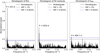 |
Fig. 3 Periodograms of HD 75 898. Left panel: GLS of the RV data. Central panel: GLS of the RV residuals after subtracting a sinusoidal with a period corresponding to the initial peak. Right panel: GLS of the stellar activity indicator SMW. |
5 HD 75898
5.1 Previous works
HD 75898 is a bright and metal-rich star about 80 pc away that was previously classified as a G0V. However, as pointed out by Robinson et al. (2007), it is more likely an F8V star that is starting to evolve along the subgiant branch. It is a bit larger and more massive than the Sun, but slightly younger. Planet b has been announced for the first time by the same authors, who also reported a long-period trend possibly indicating the presence of an additional object. The known planet has a minimum mass of ~2.5 MJ, with a period of around 420 days, and a moderate eccentricity (e = 0.1). Bryan et al. (2016) analyzed the long-term trend of this target, placing constraints on the mass and semimajor axis of a potential second planet: M = 2.8–199 My and a = 6.7–21 au. Successively, Ment et al. (2018) argued, based on periodogram analysis, that the long-period signal was due to an activity cycle. They dismissed the hypothesis of a second companion because of the similar periodicity of RV residuals and the S -index. In particular, they model the magnetic cycle with a Keplerian curve, obtaining a period of P = 6066 ± 337 d and an RV semi-amplitude of 44 ± 12 ms−1. The latter value is in strong contrast with the results obtained by Lovis et al. (2011, Fig. 19). In their work, the authors show the RV semi-amplitude induced by magnetic cycles for a sample of typical, old, solarlike stars in our neighborhood, with values ranging from 0 to about 12 m s−1 . HD 75898 is also an old, solar-like star with a temperature around 6000 K (Robinson et al. 2007), so the RV signal attributed by Ment et al. (2018) is one order of magnitude greater. This is the first hint that the observed long-term RV variation is more likely induced by the presence of a long-period giant planet rather than an activity cycle. The SMW time series of this target indeed shows a clear periodicity, and so we include it in our fit.
5.2 Periodogram analysis
We extracted the GLS to the RVs of HD 75898, finding that the signal corresponding to the known planet (~420 d) is well visible and is strongly dominant. The residuals show a peak at a period of 5555 d (FAP ≪ 0.001%), so the same order of magnitude as the signal observed by Ment et al. (2018) and mentioned in the previous section. However, in the periodogram of the activity index SMW, the highest signal is at 854 d (FAP ≲ 0.001%). Since the two peaks are at very different periods, it is more likely that the one observed for RV residuals is caused by a second planet rather than activity. However, since the peak in the GLS of the SMW is also significant, we include the activity indicator time series in our analysis to check whether stellar activity contributes to the overall RV signal on a timescale of about 854 d. The peri-odograms of the RVs, RV residuals, and S -index are shown in Fig. 3.
5.3 RV orbital fit
As previously mentioned, we used PyORBIT for the RV analysis. We set different offsets and jitters for HIRES and HARPS-N. We included a GP with a quasi-periodic kernel, following the definition of Rajpaul et al. (2015), trained on the activity indexes, in which the hyperparameter h can be seen as the activity contribution to the RV signal.
We performed different orbital fits. In the first case, we wanted to reproduce the result of Ment et al. (2018) to compare it with the other models in the Bayesian framework, so we used one Keplerian term with a quasi-periodic GP (Model 1, M1). To make sure we obtained a period on the same order of magnitude as they found, we limited the period of the GP to the range [2000, 10 000] d but we put no constraints on its contribution to the RV signal. In the second case, we used two Keplerian terms without activity: this model takes into account the possibility that, despite the signal visible in the GLS of the SMW time series, activity does not contribute to the RV signal (Model 2, M2). As boundaries, we placed the limits 2000 ≤ Pc ≤ 20 000 d and 20 ≤ Kc ≤ 80 m s−1. The choice of the boundaries on the period has been done in the following way. Since the GLS peak is at 5555 d, we expect the second planet to be at a period of a few thousand days, so we set 2000 d as the minimum. On the other hand, 20 000 d is almost 4 times the nominal peak so with this as the maximum we are still exploring a large portion of the parameter space but without going into regions where we don’t expect to find any signal, making the analysis less computationally expensive. Next, we considered the residuals of M2 and searched for a correlation with activity indicators. For this step, we only used the HARPS-N set because we have more information and details about it, while for the HIRES set we only have the SMW value. First of all, we looked at the S/N of the spectra in the 6th order, which corresponds to the spectral region where the Ca H & K lines are found. The values for this quantity range from 4.2 to 79.1, with a mean and a median of 34.3 and 32.5, respectively. This indicates that they are mostly of good quality, and therefore we did not remove any of them. We calculated the Spearman’s rank coefficient and the corresponding p-value between the SMW values and the RV residuals. These are shown in Fig. 4 with the corresponding linear best fit. In particular, we find r = 0.64, which indicates a good correlation. Furthermore, we also obtain a p-value of p = 2 × 10⁻¹⁵, proving that such a correlation is very significant. We applied the same procedure to the correlations with the Bisector Inverse Span (BIS) of the CCF as derived from the spectra with the HARPS-N pipeline. We obtain r = 0.34 and p = 10−4, indicating that there is no correlation.
As explained above, we find a significant peak in the GLS of the S -index time series and this is correlated with RVs. In addition, as shown in Fig. 5, correlated noise is visible by eye (especially in the HARPS-N data set) in our data so, following these results, we performed an additional analysis combining RVs and SMW with a model including two Keplerian terms with quasi-periodic GP: this has been done to consider both the presence of an additional long-period planet and an activity cycle (Model 3, M3). We used the same boundaries as in M2 for planet c and, in addition, we set 1 ≤ h ≤ 15 m s−1, since these values are consistent with the results of Lovis et al. (2011) mentioned before. What’s more, in our first tests, we obtained two very different offsets for the HIRES and HARPS-N SMW time series, faking a very long-term (P > 10000 d) signal. To avoid this computational problem, we limited the period of the GP to 2 ≤ Pcycle ≤ 1200 d, a range that includes the strongest peak found in the GLS. We find BIC(M1) = −247.6, BIC(M2) = −194.5, and BIC(M3) = −276.2. We consider the model selection criterion by Kass & Raftery (1995) according to which a model (A) is strongly favored over another (B) when ∆BICBA > 10. In our case, we have ∆BIC = 28.6 and 81.7 in favor of M3 compared to M1 and M2, respectively, and therefore conclude that there is strong evidence that Model 3 is the most convincing representation of the actual RV data. The nominal period obtained for the putative second planet is slightly lower (18.3 yr vs 19.3 yr) than the time span covered by our data set, meaning that we have a full-phase coverage of its orbit. As a final step, we extracted the GLS of the RV residuals from Model 3. The nominal highest peak is at a period of 17 d but with FAP= 34%, indicating that there are no other significant signals in our time series. However, since the GLS assumes zero eccentricity, one cannot rule out the presence of additional planets on eccentric orbits. Thus, we fitted our data with another model (Model 4, M4) including a third planet in addition to Model 3. We obtain BIC(M4) = −236.8 and so ∆BIC = 39.4 in favor of M3, indicating once again that this model is to be preferred. With these results, we find that the total RV signal is explained by the known planet of the system, a new companion to be named HD 75898 c, and an activity cycle with an intermediate period (~800 d). The final parameters of the best fit are shown in Table 5.
 |
Fig. 4 Chromospheric activity indicator and RV residuals obtained from a model without GP, and corresponding linear best fit. |
5.4 Orbital parameters and true mass of HD 75898 c
We used the DE-MCMC algorithm described in Sect. 4.3 to fit the combined PMA+RV model to the HIPPARCOS-Gaia absolute astrometry of HD 75898 reported in Table 3 and to the offset-corrected RV dataset from which the signal of HD 75898 b had been removed. The choice is justified by the fact that, as shown in Fig. 6, the inner planet falls in the region of significantly reduced sensitivity of the PMA technique, given its orbital period and minimum mass. We therefore assumed that the combined analysis can only constrain the orbit and mass of the outer companion, HD 75898 c. From Fig. 6 we also see that, at the separation of HD 75898 c its minimum mass falls below the PMA sensitivity curve. The low significance (S/N~ 2) of the PMA should then possibly indicate that the true mass of HD 75898 c is higher than its m sin i value. This is indeed what we found in our analysis.
Table 6 reports the best-fit orbital solution for HD 75898 c in the case of both a prograde and a retrograde direction of motion7. We derive  deg and
  deg for a pro-grade and retrograde orbit, respectively. The fitted mass ratio, qc = 0.0063 ± 0.0005 (for the prograde orbit), implies a (derived) true mass of
  MJup. For the case of the prograde orbit, the joint posteriors of these parameters are shown in Fig. A.1 while Fig. A.2 shows the best-fit orbital solution superposed to the observational data.
Assuming coplanarity, the true mass of HD 75898 b might be closer to 6 MJup, not yet sufficient to produce any detectable perturbation in the HIPPARCOS-Gaia absolute astrometry, as seen in Fig. 6. Following Sozzetti (2023), we performed a sensitivity analysis of Gaia DR3 astrometry to companions of a given mass and orbital separation based on the RUWE (Renormal-ized Unit Weight Error) statistic (Lindegren et al. 2021). This quantity corresponds to the square root of the reduced χ2 of the single-star fit to the along-scan observations normalized by an empirical scaling factor that depends on G magnitude and the color index GBP + GRP in order to account for calibration errors. In this way, well-behaved stars will have RUWE ≈ 1.0 (see Lindegren et al. 2021 for details). The RUWE value of 0.93 for HD 75898, as reported in the Gaia archive, therefore implies a single-star model suffices to describe the variability in the Gaia DR3 astrometric time series. Indeed, as shown in Fig. 6, at the orbital separation of HD 75898 b, only companions with a mass ~10 times larger than its minimum mass would have had a high chance of producing excess residuals in Gaia DR3 astrometry, and therefore a RUWE larger than the measured one. Thus, we are not able to make any meaningful statements on the possible relative alignment between the orbits of the two planets.
 |
Fig. 5 Chromospheric activity indicator time series and best-fit solution of the Gaussian Process with quasi-periodic kernel. Table 5 – Planetary parameters obtained from the RV analysis using full-Keplerian models. |
Planetary parameters obtained from the RV analysis using full-Keplerian models.
 |
Fig. 6 HIPPARCOS-Gaia PMA and Gaia DR3 sensitivity to companions of a given mass (in MJup) as a function of the orbital semi-major axis (in au) orbiting HD 75898. Dashed, dashed-dotted, and long-dashed lines correspond to iso-probability curves for 50, 90, and 99% probability of a companion of given properties to produce RUWE > 0.93. The solid black line identifies the combinations of mass and separation explaining the observed astrometric acceleration at the mean epoch of Gaia DR3 (based on the analytical formulation of Kervella et al. 2019). The shaded light-blue region corresponds to the 1σ uncertainty domain. The black star and red hexagon indicate the m sin i value (from RVs only) and the true mass value (combining RVs with astrometry, prograde orbit case) for HD 75898 c obtained in this work, respectively. The black cross identifies the location of HD 75898 b. |
Orbital parameters and true mass for HD 75898 c from the combined RV+astrometry analysis.
6 HD 11506
6.1 Previous works
HD 11506 is very similar to the previous target in mass and metallicity but is slightly younger and less evolved. It is located at a distance of about 50 pc and is classified as a G0V star. This star is already known to host two planets. The first one was announced by Fischer et al. (2007), who obtained an orbital period of around 1400 days and a minimum mass of 4.74 MJ. They also reported several peaks in the periodogram of the residuals, suggesting the presence of at least one additional companion. A couple of years later, Tuomi & Kotiranta (2009) analyzed the system and obtained significantly different results, as they reported a period of 3.48 yr (1270 d) and a minimum mass of 3.44 MJ for planet b. They also announced a second planet with P = 0.467 yr = 170 d and m sin i = 0.82 MJ. Interestingly, they find a rather high eccentricity of e = 0.42 for this second planet. Giguere et al. (2015) used a larger data set to better constrain the parameters of these two planets, obtaining Pb = 1627.5 d, mb sin ib = 4.21 MJ, Pc = 223.6 d, and mc sin ic = 0.36 MJ. They also reported the presence of a linear trend suggesting that another long-period planet might be present. Such a linear trend has been quantified as −7.4 ± 0.47 m s−1 /yr by Bryan et al. (2016). Their constraints on the mass and semi-major axis of the external planet are M = 9.6–72 MJ and a = 14–40 au. Both Fischer et al. (2007) and Giguere et al. (2015) investigated the activity index SMW and found that, for this object, activity does not have a significant impact on radial velocities. Recently, Feng et al. (2022) announced the discovery of a third planet in this system, with a period of about 14 700 days and a mass of 7.38 MJ. These values have been obtained by combining the HIPPARCOS-Gaia absolute astrometry with their RV data set. Thanks to our larger RV dataset from HARPS-N observations, we can put additional constraints on the mass and period of planet d.
6.2 Periodogram analysis
The periodogram of the RVs of HD 11506 shows the peak corresponding to planet b, which is around 1700 d, and a significant signal at long periods. After removing a sinusoidal term with a 1700 d period, we find a new peak at 826 d that does not correspond to planet c. This is close to half the orbital period of planet b and it is not surprising because we removed a signal corresponding to a circular orbit while planet b has a significant eccentricity. After removing this additional signal, the residuals show a peak corresponding to planet c (223 d, FAP ≪0.001%) and, again, additional residual power at long periods.
6.3 RV orbital fit
For this object, we used three different offset and jitter terms: HIRES pre-upgrade, HIRES post-upgrade, and HARPS-N (as described in Sect. 2.1.2). We fitted our data with three Keplerian terms. As mentioned, previous works demonstrated that no activity cycles are affecting RVs for this target. As a first test, we included activity in our analysis using a GP with a quasi-periodic kernel but we immediately confirmed that it did not give an important contribution to the RV signal: the hyperparameter h was always compatible with zero within 1σ and the period was highly unconstrained. Therefore, we excluded the SMW time series from the subsequent models.
Unfortunately, in the best-fit solution, the period of the putative third planet turns out to be highly unconstrained as our data cover only ~33% of the nominal period value. For this reason, we tried two more models with linear and quadratic trends instead of the third Keplerian. In both cases, the parameters obtained for the two known planets are compatible with each other and the literature. In the former case, we obtain a linear coefficient of  , which allows us to make a rough estimate of the minimum mass and period. Since the observed slope covers, at best, half of the height between the RV maximum and minimum (considering low-eccentricity orbits), we can calculate
 (1)
(1)
where AT is the length of the time baseline. In addition, AT can be at most about one-quarter of the orbital period, so we can estimate this as P ≥ 4 ⋅ ∆T. Then, we can find the minimum mass as
 (2)
(2)
with Ms mass of the star in solar units, K is the RVs semiamplitude of the planet in m s−1 and P period of the planet in years. In this case, we obtain Pd ≥ 27579 days, Kd ≥ 125 m s−1, and therefore md sin id ≥ 21.25 MJ. Both the period and the minimum mass are compatible with the ones obtained with the Keplerian orbit. Both results show that this should be a Brown Dwarf (BD) rather than a planet.
Similarly, we can make a guess using the results of the fit with the quadratic trend, from which we obtained  and
and  . We can estimate the amplitude as the difference between the maximum and minimum value of RVs, that is K ≥ RVmax − RVmin. For the period, we use the expression derived by Kipping et al. (2011):
 (3)
(3)
In this case, we obtain Kd ≥ 130 m s−1, Pd ≥ 234 yr, and therefore md sin id ≥ 32.14 MJ, which is far greater than the previous two values (Keplerian and linear models). This period corresponds to ~234 years or ~40.2 au, making it an extremely distant object, and we believe that this is probably an overestimate. What’s more, a minimum mass of ~32 MJ is in contrast with the results shown in Fig. 1. In particular, at these orbital separations, the SPHERE nondetection should exclude companions with m ≳ 30 MJ.
We now point out that the BICs are 1385 for the 3-planets model, 1292 for the 2-planets + linear trend model, and 1278 for the 2-planets + quadratic trend model, so that the last model is to be favored. These three are shown together in Fig. 7. As we can see, the three models are very hard to distinguish because there is almost no curvature in this trend. We conclude that, with RVs alone, we cannot reach a definitive conclusion on the nature of this third object at present. The results obtained with the three Keplerian terms are shown in Table 5.
As a final check, we performed the same analysis as the previous target, searching for a correlation between RV residuals and activity indicators. In particular, we used the residuals obtained from the model with three Keplerians and, as done before, we only used the HARPS-N dataset. As we can see in Fig. 8, two points are clear outliers. The leftmost one was taken on 3 January 2022 and differs by 8σ from the mean of the whole time series. It has S/N = 4, the lowest of the dataset, and an RV error bar of 10 m s−1, the highest of all. After removing this point, we considered the other one, taken on 24 November 2015. For this observation, we have S/N = 4.9 and an RV uncertainty of 8.4 m s−1, the second lowest and highest of the time series, respectively. In addition, it differs by about 4σ from the mean (recalculated after removing the first outlier). Upon removal of these two data points, we calculated Spearman’s rank coefficient, obtaining r = 0.37, indicating no correlation and confirming that does not seem to contribute to the RV signal. Additionally, we extracted the GLS of the RV residuals and found a nominal highest peak at 173 d with FAP = 0.5%. This FAP is not low enough to motivate the search for an additional planet at this period. What’s more, as shown in Sect. 6.6, a planet with such a period is very unlikely to be present as it would be very close to planet c.
 |
Fig. 7 Keplerian, linear, and quadratic models for the RVs of HD 11506 after subtracting the two known planets. |
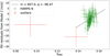 |
Fig. 8 Chromospheric activity indicators and RV residuals obtained from a three-planet model without accounting for stellar activity and corresponding linear best fit (obtained after removing the two outliers). |
6.4 Orbital parameters and true mass of HD 11506 d from combined fits
As in the case of the HD 75898 system, we ran the DE-MCMC analysis with the PMA+RV model fitted to the HIPPARCOS-Gaia absolute astrometry of HD 11506 from Table 3 and the offset-corrected RV dataset with the signals of both HD 11506 b and HD 11506 c removed. On the one hand, the orbital separation of the former companion, just below 3 au, places it close to the region of highest sensitivity of the PMA technique, as shown in Fig. 9. However, its minimum mass is still significantly lower than the one required in order to be compatible with the clearly detected (S/N~ 6) astrometric acceleration. On the other hand, the inferred intervals of minimum mass and orbital semi-major axis for HD 11506 d based on the tentative RV orbit presented in the previous section are compatible with the observed PMA being entirely due to the effect of orbital motion induced by the outermost companion, presumably with a true mass close to its minimum and therefore with an inclination not far from 90 deg.
We report in Table 7 the best-fit orbital solution for HD 11506 d. Despite only seeing a long-term trend in the RV data covering ~30% of the period, we can set precise constraints on the orbital parameters of the companion. In particular, we obtain an inclination  deg, which is compatible with an almost perfectly edge-on configuration. We determine a mass ratio
  , corresponding to a true mass of
  MJup, exactly at the commonly used mass thresh- . old used to distinguish planets from brown dwarfs. The results fully confirm the initial assumption that the observed PMA is dominated by the contribution to orbital motion effects due to HD 11506 d. The joint posteriors of the parameters mentioned above are shown in Fig. A.3, while Fig. A.4 shows the best-fit orbital solution superposed to the observational data. We do note that the formally very precise combined solution we obtain is surprising. In similar cases studied in the recent past, such as the 14 Her system (Bardalez Gagliuffi et al. 2021 and Benedict et al. 2023), uncertainties in the orbital parameters and true mass for the outermost companion with only partial phase coverage are significantly larger. One possible reason could be due to our choice to model the combination of RVs and absolute astrometry only for HD 11506 d, with the contributions from the inner two planets subtracted. Given the data at hand, we stress the orbital solution for HD 11506 d should be regarded as preliminary.
The Gaia archive entry for HD 11506 reports RUWE = 1.27. The threshold for establishing a clear departure from a good single-star fit to Gaia-only astrometry is usually placed at 1.40 (e.g., Lindegren et al. 2018, 2021). While we cannot claim strong evidence of orbital motion in the Gaia DR3 astrometry of HD 11506, the sensitivity analysis (see Fig. 9) shows that there is ~ 50% probability that the observed RUWE is due to orbital effects induced by HD 11506 b, and the likelihood increases if its true mass were to be larger than the m sin i value. This would imply a possible departure from coplanarity with (at least) HD 11506 d. We explored this possibility by performing a combined fit of the PMA data with the RV signals ofHD 11506 b and HD 11506 d, removing from the RV datasets only the signal of HD 11506 c. Indeed, we obtained a solution statistically favored with respect to that of the 1-planet combined fit (log-likelihood In ℒ = −95 and In ℒ = -104 for the 2-planet and 1-planet fit, respectively). The orbital elements and mass of HD 11506 d remained essentially indistinguishable from those reported in Table 7, while for HD 11506 b we obtained ib = 31 ± 7 deg, Ωb = 116 ± 22 deg, and mb = 9 ± 2 MJup. This translates into a mutual inclination angle irel = 80 ± 11 deg. As we discuss in the following section, such a strong degree of misalignment between planet b and d implies dynamical instability and system disruption on short time-scales, independent of the orbital alignment and true mass of planet c. We attempted to force orbital solutions with much longer orbital periods for HD 11506 d (up to 250 yr), but the DEMCMC analysis never reached convergence (i.e.,good mixing of the chains). We therefore interpreted the favorable outcome of the two-planet combined orbital fit as a result of overfitting the PMA data, and decided to keep the (preliminary) solution presented in Table 7 as baseline.
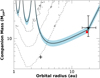 |
Fig. 9 HIPPARCOS-Gaia PMA and Gaia DR3 sensitivity to companions of a given mass (in MJup) as a function of the orbital semi-major axis (in au) orbiting HD 11506. Dashed, dashed-dotted, and long-dashed lines correspond to iso-probability curves for 50, 90, and 99% probability that a companion of given properties will produce RUWE > 1.27. The solid black line identifies the combinations of mass and separation explaining the observed astrometric acceleration at the mean epoch of Gaia DR3 (based on the analytical formulation of Kervella et al. 2019). The shaded light-blue region corresponds to the 1σ uncertainty domain. The black star and red hexagon indicate the m sin i value(from RVs only) and the true mass value (combining RVs with astrometry) for HD 11506 d obtained in this work, respectively. The black cross identifies the location of HD 11506 b. |
Orbital parameters and true mass for HD 11506 d from the combined RV+astrometry analysis.
6.5 Orbital stability of misaligned system architectures
The identification of a potential orbital solution on which planet b and d have highly misaligned orbits calls for a dedicated check of the orbital stability of this configuration, considering the rather large planetary masses, the moderately large eccentricity of planet b and the presence of the additional planet c. The direct N-body numerical integration of the system over 50 Myr for increasing values of the inclination ib of planet b shows that for values of ib higher than 35–40 deg the planetary system becomes unstable. A period of chaotic evolution, caused by repeated mutual close encounters, follows until a collision with the star or another planet or the ejection from the system of one body occurs. This behavior is shown in Fig. 10 where the timescale for the onset of instability is computed for different values of ib . The initial values of the remaining orbital angles are selected randomly (together with the nominal ones) to make the exploration more general. We conclude that the possibility that planet b is on a highly inclined orbit with respect to the orbital plane of the other two planets is excluded by dynamical reasons.
6.6 The complex dynamics of the system
To further investigate the stability of the system in the assumption of low mutual inclinations of the planetary orbits we have used the FMA (Frequency Map Analysis, Laskar 1993, Šidlichovský & Nesvorný 1996). This method allows us to quantitatively measure the stability of an orbit by determining the diffusion rate of intrinsic dynamical frequencies of the planetary system in the Fourier space. We tested the variation of the main secular frequency g of the inner planet over a timescale of 10 Myr (g is of the order of 105 yr) and computed its diffusion rate as f = − log10(σg/g) where σg is the standard deviation of the frequency g computed over running windows of 106 yr spanning the full numerical integration. The lower the value of f the more stable is the planetary system since its fundamental frequencies are constant. We sampled different initial dynamical configurations close to the nominal one by varying the semi-major axis of the outer planet from 17.7 to 18.7 au and the inclination of the inner planet up to 25 deg. The other orbital angles of the two inner planets have been randomly selected between 0 and 2π while those of the outer planet have been kept constant. The outcome of the FMA analysis is shown in Fig. 11. Configurations with high (yellow to red) and low changes (blue to black) in the frequency are mixed up implying that chaotic and quasistable solutions are dense within each other. This is surprising because, in this kind of analysis, it is typically expected to find an extended area of stable motion possibly surrounded by chaotic regions. A very similar result has been obtained by using as chaos indicator MEGNO (the Mean Exponential Growth factor of Nearby Orbits; Cincotta & Simó 2000 and Gozdziewski et al. 2001) closely related to the maximum Lyapunov exponent.
This peculiar behavior is due to the strong secular perturbations of the outer planets on the inner one which can pump up its eccentricity to values as high as 0.65. High values of eccentricity easily lead to a chaotic evolution and explain why, for different initial values of the pericenter longitudes (ϖ), the behavior is more or less chaotic. Since, in our sampling procedure, the orbital angles are chosen randomly, it is expected that stable systems (low eccentricity) are mixed up with chaotic ones (high eccentricity). For example, in Fig. 12 the semi-major axis evolution of the inner planet is shown for different initial values of the planet ϖ. In the first case, the maximum eccentricity is 0.25 (the lowest value of eccentricity due to the secular perturbations and compatible with the nominal configuration) and the variation of the secular frequency is f = 4 × 10⁻⁶ while in the second case, the maximum eccentricity is about 0.65 (the highest value) and the secular frequency variation is f = 3 × 10⁻⁴. The semi-major axis in the low eccentricity case is stable and periodic while in the high eccentricity case it shows random changes suggestive of a chaotic nature confirmed by the higher value of f.
However, this chaotic nature does not seem to lead to instability on a short timescale. The direct numerical integration of the nominal system over 3 Gyr (see Fig. 13), where a small orbital inclination of 1° is assumed for the two inner planets, shows a chaotic evolution but the system remains stable. This may be a case of “stable chaos” (as described in Milani & Nobili 1992 and Gayon et al. 2008) where the unstable region is bounded and the chaotic wandering does not lead to close encounters with one of the other two planets. The chaotic evolution is evident from the random jumps both in semi-major axis and eccentricity but the system is stable at least over 4.5 Gyr.
This dynamical behavior may be a consequence of the initial evolution of the system. One or more additional planets in the system, subsequently ejected after a period of planet-planet scattering, may have dynamically heated the system explaining the high eccentricities and therefore the strong secular perturbations.
 |
Fig. 10 Lifetime of the planetary system for different values of the inclination of planet b (the mass is changed accordingly). The time span of the integration is 50 Myr and random initial orbital angles (mean anomaly, pericenter argument, and nodal longitude) have been adopted in addition to the nominal ones in order to make the exploration more complete. The green dot represents the nominal case. For inclinations higher than 30–40 deg, the system becomes unstable on a timescale of shorter than 50 Myr. |
 |
Fig. 11 Diffusion portrait of the secular frequency g of the inner planet for different initial values of its inclination (y-axis) and of the semimajor axis of the outermost planet. The different color levels mark the value of f, the negative value of the logarithm of the relative dispersion of the secular frequency g. Smaller values of f correspond to more stable systems. |
7 Discussion
7.1 Detection limits for additional planets
We tested the presence of additional RV planetary companions around the two stars, deriving the detection limits from the combined RV datasets. We performed injection-recovery simulations to compute the detection functions for each system. We followed a procedure similar to those performed in Bonomo et al. (2023) and Naponiello et al. (2023); in addition, to correctly take into account the effects of the stellar activity cycle, we injected the simulated signals in the real RV data, after correcting for instrumental offsets, and then tested the recovery by comparing the BIC of the final RV models (see Table 5) to that obtained by adding the simulated planetary signal, thus including the GP regression in the analysis. We performed this analysis in a logarithmic grid of 80 × 70 in minimum mass and orbital period, respectively, covering the ranges [1, 3 × 10³] M⊗ and [1,104] d.
The resulting detection maps are shown in Fig. 14. As the dynamical analysis from Sect. 6.6 did not point out any preferred stability regions, we tested the limits on the presence of undetected short-period companions, in the two intervals [1,10] d, and [10,100] d as shown by the highlighted regions in Fig. 14. The 90% detection threshold for HD 75898 are Mp sin i > 16.5 M⊗ and Mp sin i > 36.7 M⊗ for [1,10] d and [10,100] d, respectively. For HD 11506 the detection thresholds are Mp sin i > 8.3 M⊗ and Mp sin i > 16.5 M⊗ for [1,10] d and [10, 100] d, respectively.
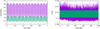 |
Fig. 12 Evolution of the inner planet eccentricity (left panel) for two different initial values of ϖ. The corresponding evolution of the semi-major axis, over a longer timescale, is illustrated on the right panel. The higher eccentricity case shows chaotic behavior. |
 |
Fig. 13 Long-term evolution (4.5 Gyr) of the nominal planetary system. The eccentricity is shown on the right panel. Here, the lower limit on the vertical axis has been set to outline the chaotic evolution. |
7.2 Gaia DR4 simulations
The mutual inclination between the planetary orbits is one of the most important parameters in the study of multiple systems. As discussed in Sect. 6.6, different mutual inclinations can greatly change the stability of the system and, moreover, the relative orientation of the orbits is one of the driving factors in many dynamical interaction mechanisms such as the Lidov-Kozai effect (Lidov 1962; Kozai 1962). However, the only information concerning the orbital orientation of the studied systems comes from the PMA analyses of the outer planets (see Sects. 5.4 and 6.4), the inner planets, observed only with RVs, have no information on their inclinations. This ambiguity could be solved with time-series astrometry from Gaia. However, to date, Gaia DR3 has not found any orbital solutions for companions around either HD 75898 orHD 11506. Therefore we decided to perform a series of numerical simulations to test whether some of the planets in the systems could be detected by the future Gaia DR4.
We followed a similar setup to Sozzetti et al. (2023), acquiring the transit information from the Gaia Observation Forecast Tool (GOST)8, and the stellar motion five-parameter solution from Gaia DR3 (see Table 4). We simulated separately each of the planets in the two systems, taking the RV orbital parameters from Table 5. For each planet, we generated 100 astrometric time series, with the longitude of the ascending node, Ω, drawn from a uniform distribution [0, π], and the inclination, i, drawn from a uniform distribution of cos i ∈ [−1,1]. Each time series was fitted with a 12-parameter stellar-motion + orbital motion partly linearized model, using the emcee Affine Invariant MCMC Ensemble sampler by Foreman-Mackey et al. (2013). We performed a blind search, to test whether the signal could be recovered by the astrometric data alone. The full results of these analyses for each planet are shown in detail in Appendix B, here we shall discuss the main features.
Of the two planets orbiting HD 75898, neither was significantly detected in the simulated astrometric time series: HD 75898 b has a too small projected semi-major axis, 〈a〉 ≃4 0 µas; HD 75898 c instead has an orbital period of more than three times longer than Gaia DR4 timespan, and thus cannot be significantly recovered from the astrometric data alone. HD 11506 shows instead some promising features: the injected astrometric signal of planet b is significantly (ΔBIC < –10) recovered 47% of the times and, as shown in Fig. 15, the fitted values of i and Ω are very close to the input values. It is worth noting that we based these simulations on the current noise levels for Gaia DR3 for stars of similar magnitude (i.e., σw = 0.1 mas Holl et al. 2023), while the noise level for DR4 is expected to be significantly lower, thus improving the recovery rate of the planet’s astrometric signal. The signal of HD 11506 c instead is not recovered in any of the simulated time series, as due to its short period and low mass, it has a median projected semi-major axis of 6 µas, well below the noise threshold. Planet d instead has an orbital period more than 10 times longer than the DR4 time span, and thus cannot be recovered as an orbital motion. However, as discussed in Sect. 6.4, the orbit of HD 11506 d can be recovered with good precision with the combination of RVs and PMA analysis, and thus the orientation of the orbit (e.g., id and Ωd) is already known: this means that if, as expected, the astrometric signal of planet b is recovered in Gaia DR4, it will be possible to determine the relative inclination of the two planets.
 |
Fig. 14 Detection function maps of the RV time-series of HD 75898 (upper panel) and HD 11506 (lower panel). The gray-scale indicates the detection probability in the orbital period – minimum mass parameter space. The planets orbiting the two stars are shown as red dots. The colored regions show the intervals of periods investigated for additional planets, while the dotted lines mark the respective 90% detection thresholds. |
8 Conclusion
In this paper, we analyze two well-known solar-like stars, namely HD 75898 and HD 11056. Both were already known to host planets, with evidence of long-term RV signals.
For HD 75898, we demonstrate that the activity cycle mentioned by Ment et al. (2018) includes the contribution of a second massive planet and a medium-period activity cycle with a contribution to the RV signal similar to that of the Sun. Thanks to the combination of full-phase coverage with RV data and astrometry, we are able to put precise constraints on the mass and orbital parameters of this new candidate.
For HD 11506, we confirm the candidate presented by Feng et al. (2022); however, thanks to a larger RV data set, we demonstrate that the reported mass and period for this object are likely underestimated. Once again, the combination of RVs and astrometry allows us to constrain the mass and period of this object in a way that would not be possible with RVs alone due to the very long period. We also illustrate the peculiar dynamic situation of this system with three gaseous planets, of which at least two have large masses, which makes it a very interesting science case.
We would like to stress the importance of long-term RV monitoring with high-accuracy instruments like HARPS, HARPS-N, and HIRES, which remain stable over several years, because, as shown, these can bring scientific results of great value. This becomes even more important considering the synergy between RVs, astrometry, and direct imaging when detecting long-period planets. Unfortunately, planets at wider orbital separations are more difficult to study, unless they are very young and massive. However, studying this part of the parameter space is essential in order to gain a complete understanding of these planetary systems. In this context, maintaining stable high-resolution instruments active is of vital importance for the whole exoplanetary community.
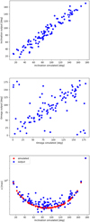 |
Fig. 15 Gaia astrometry simulation results for HD 11506 b. Top panel: derived inclination vs. simulated value. Middle panel: derived longitude of the ascending node vs. simulated value. Bottom panel: derived (blue) and simulated (red) astrometric semimajor axis vs injected orbital inclination. |
Data availability
The full HARPS-N RV time series are available at the CDS via anonymous ftp to cdsarc.cds.unistra.fr (130.79.128.5) or via https://cdsarc.cds.unistra.fr/viz-bin/cat/J/A+A/689/A235
Acknowledgements
This work has made use of data from the European Space Agency (ESA) mission Gaia (https://www.cosmos.esa.int/gaia), processed by the Gaia Data Processing and Analysis Consortium (DPAC, https://www.cosmos.esa.int/web/gaia/dpac/consortium). Funding for the DPAC has been provided by national institutions, in particular the institutions participating in the Gaia Multilateral Agreement. A.S. and M.P. acknowledge support from the Italian Space Agency (ASI) under contract 2018-24- HH.0 “The Italian participation in the Gaia Data Processing and Analysis Consortium (DPAC)” in collaboration with the Italian National Institute of Astrophysics. We acknowledge the financial support of the European Union – NextGenerationEU (RRF M4C2 1.1 PRIN 2022, Project 20229R43BH) and the “Programma di Ricerca Fondamentale INAF 2023” of the National Institute of Astrophysics (Large Grant 2023 EXODEMO). SPHERE is an instrument designed and built by a consortium consisting of IPAG (Grenoble, France), MPIA (Heidelberg, Germany), LAM (Marseille, France), LESIA (Paris, France), Laboratoire Lagrange (Nice, France), INAF – Osservatorio di Padova (Italy), Observatoire de Genève (Switzerland), ETH Zurich (Switzerland), NOVA (Netherlands), ONERA (France), and ASTRON (Netherlands), in collaboration with ESO. SPHERE was funded by ESO, with additional contributions from CNRS (France), MPIA (Germany), INAF (Italy), FINES (Switzerland), and NOVA (Netherlands). SPHERE also received funding from the European Commission Sixth and Seventh Framework Programs as part of the Optical Infrared Coordination Network for Astronomy (OPTICON) under grant number RII3-Ct-2004-001566 for FP6 (2004–2008), grant number 226604 for FP7 (2009–2012), and grant number 312430 for FP7 (2013–2016) This work has made use of the SPHERE Data Centre, jointly operated by OSUG/IPAG (Grenoble), PYTHEAS/LAM/CeSAM (Marseille), OCA/Lagrange (Nice), Observatoire de Paris/LESIA (Paris), and Observatoire de Lyon, also supported by a grant from Labex OSUG@2020 (Investissements d’avenir – ANR10 LABX56).
Appendix A Orbital solutions and posterior distributions
Fig. A.1 shows joint posteriors for relevant parameters only constrained by the PMA+RV combination (inclination, longitude of the ascending node, true mass) in the case of HD 75898 c. Fig. A.2 shows the best-fit Keplerian solution superposed to the RV time series and the calibrated HIPPARCOS and Gaia proper motions. Fig. A.3 and Fig. A.4 show the same information in the case of HD 11506 d.
 |
Fig. A.1 Joint posterior distributions for inclination, longitude of the ascending node and true mass for HD 75898 c. |
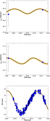 |
Fig. A.2 Best-fit orbital solution (solid black line) for HD 75898 c, superposed to the calibrated proper motions from HIPPARCOS and Gaia (top and middle panels) and to the RV time series (bottom panel). The dashed orange lines represent random selections of orbital solutions drawn from the posterior distributions. |
 |
Fig. A.3 Joint posterior distributions for inclination, longitude of the ascending node and true mass for HD 11506 d. |
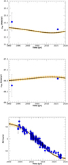 |
Fig. A.4 Best-fit orbital solution (solid black line) for HD 11506 d, superposed to the calibrated proper motions from HIPPARCOS and Gaia (top and middle panels) and to the RV time series (bottom panel). The dashed orange lines represent random selections of orbital solutions drawn from the posterior distributions. |
Appendix B Gaia DR4 simulations: results
Here we showcase all the results for the Gaia DR4 astromet-ric time series simulations discussed in Sect. 7.2. Figures B.1 and B.2 show the results for the analyses of the two planets orbiting HD 75898: as can be seen from the two top panels of both figures, in neither case it is possible to correctly recover the orientation of the orbits; in the case of planet b, it is because the amplitude of the signal is below the noise level, σw = 0.1 mas, as shown in the bottom panel; on the other hand for planet c, while the amplitude of the signal would be more than significant (see bottom panel of Fig. B.2), it cannot be recovered due to its too long period compared to the 66-month timespan of Gaia DR4.
The results for HD 11506 c and HD 11506 d are shown in Figs. B.3 and B.4. HD 11506 c has an even lower astrometric amplitude than HD 75898 b, and thus cannot be detected in the simulated time series, while the even longer period of HD 11506 d compared to HD 75898 c also makes it impossible to detect as a Keplerian orbit in the data (as discussed in Sect. 7.2).
 |
Fig. B.1 Gaia astrometry simulations results for HD75898 b. Top panel: derived inclination vs simulated value; middle panel: derived longitude of the ascending node vs simulated value; bottom panel: derived (blue) and simulated (red) astrometric semimajor axis vs injected orbital inclination. |
 |
Fig. B.2 Gaia astrometry simulations results for HD75898 c. Top panel: derived inclination vs simulated value; middle panel: derived longitude of the ascending node vs simulated value; bottom panel: derived (blue) and simulated (red) astrometric semimajor axis vs injected orbital inclination. |
 |
Fig. B.3 Gaia astrometry simulations results for HD 11506 c. Top panel: derived inclination vs simulated value; middle panel: derived longitude of the ascending node vs simulated value; bottom panel: derived (blue) and simulated (red) astrometric semimajor axis vs injected orbital inclination. |
 |
Fig. B.4 Gaia astrometry simulations results for HD 11506 d. Top panel: derived inclination vs simulated value; middle panel: derived longitude of the ascending node vs simulated value; bottom panel: derived (blue) and simulated (red) astrometric semimajor axis vs injected orbital inclination. |
References
- Allard, F., Guillot, T., Ludwig, H.-G., et al. 2003, IAU Symp., 211, 325 [Google Scholar]
- Barbato, D., Bonomo, A. S., Sozzetti, A., & Morbidelli, R. 2018, arXiv e-prints [arXiv: 1811.08249] [Google Scholar]
- Bardalez Gagliuffi, D. C., Faherty, J. K., Li, Y., et al. 2021, ApJ, 922, L43 [NASA ADS] [CrossRef] [Google Scholar]
- Benatti, S., Damasso, M., Desidera, S., et al. 2020, A&A, 639, A50 [NASA ADS] [CrossRef] [EDP Sciences] [Google Scholar]
- Benedict, G. F., McArthur, B. E., Nelan, E. P., & Bean, J. L. 2023, AJ, 166, 27 [NASA ADS] [CrossRef] [Google Scholar]
- Bensby, T., Feltzing, S., & Oey, M. S. 2014, A&A, 562, A71 [NASA ADS] [CrossRef] [EDP Sciences] [Google Scholar]
- Beuzit, J. L., Vigan, A., Mouillet, D., et al. 2019, A&A, 631, A155 [NASA ADS] [CrossRef] [EDP Sciences] [Google Scholar]
- Biazzo, K., D’Orazi, V., Desidera, S., et al. 2022, A&A, 664, A161 [NASA ADS] [CrossRef] [EDP Sciences] [Google Scholar]
- Blanco-Cuaresma, S., Soubiran, C., Heiter, U., & Jofré, P. 2014, A&A, 569, A111 [CrossRef] [EDP Sciences] [Google Scholar]
- Bonomo, A. S., Dumusque, X., Massa, A., et al. 2023, A&A, 677, A33 [NASA ADS] [CrossRef] [EDP Sciences] [Google Scholar]
- Brandt, T. D. 2021, ApJS, 254, 42 [NASA ADS] [CrossRef] [Google Scholar]
- Bressan, A., Marigo, P., Girardi, L., et al. 2012, MNRAS, 427, 127 [NASA ADS] [CrossRef] [Google Scholar]
- Bryan, M. L., Knutson, H. A., Howard, A. W., et al. 2016, ApJ, 821, 89 [NASA ADS] [CrossRef] [Google Scholar]
- Butler, R. P., Vogt, S. S., Laughlin, G., et al. 2017, AJ, 153, 208 [Google Scholar]
- Carolo, E., Desidera, S., Gratton, R., et al. 2014, A&A, 567, A48 [NASA ADS] [CrossRef] [EDP Sciences] [Google Scholar]
- Casali, G., Spina, L., Magrini, L., et al. 2020, A&A, 639, A127 [NASA ADS] [CrossRef] [EDP Sciences] [Google Scholar]
- Castelli, F., & Kurucz, R. L. 2003, ASP Conf. Ser., 210, A20 [NASA ADS] [Google Scholar]
- Cincotta, P. M., & Simó, C. 2000, A&AS, 147, 205 [NASA ADS] [CrossRef] [EDP Sciences] [Google Scholar]
- Claudi, R. U., Turatto, M., Gratton, R. G., et al. 2008, Proc. SPIE Conf. Ser., 7014, 70143E [NASA ADS] [CrossRef] [Google Scholar]
- Cosentino, R., Lovis, C., Pepe, F., et al. 2012, SPIE Conf. Ser., 8446, 84461V [Google Scholar]
- Covino, E., Esposito, M., Barbieri, M., et al. 2013, A&A, 554, A28 [NASA ADS] [CrossRef] [EDP Sciences] [Google Scholar]
- Dalba, P. A., Kane, S. R., Howell, S. B., et al. 2021, AJ, 161, 123 [NASA ADS] [CrossRef] [Google Scholar]
- Delorme, P., Meunier, N., Albert, D., et al. 2017, in SF2A-2017: Proceedings of the Annual meeting of the French Society of Astronomy and Astrophysics, eds. C. Reylé, P. Di Matteo, F. Herpin, E. Lagadec, A. Lançon, Z. Meliani, & F. Royer, Di [Google Scholar]
- Desidera, S., Sozzetti, A., Bonomo, A. S., et al. 2013, A&A, 554, A29 [NASA ADS] [CrossRef] [EDP Sciences] [Google Scholar]
- Desidera, S., Chauvin, G., Bonavita, M., et al. 2021, A&A, 651, A70 [EDP Sciences] [Google Scholar]
- Dietrich, J., & Ginski, C. 2018, A&A, 620, A102 [NASA ADS] [CrossRef] [EDP Sciences] [Google Scholar]
- Dohlen, K., Langlois, M., Saisse, M., et al. 2008, SPIE Conf. Ser., 7014, 70143L [Google Scholar]
- D’Orazi, V., Oliva, E., Bragaglia, A., et al. 2020, A&A, 633, A38 [NASA ADS] [CrossRef] [EDP Sciences] [Google Scholar]
- Doyle, A. P., Davies, G. R., Smalley, B., Chaplin, W. J., & Elsworth, Y. 2014, MNRAS, 444, 3592 [Google Scholar]
- Dumusque, X., Lovis, C., Ségransan, D., et al. 2011, A&A, 535, A55 [NASA ADS] [CrossRef] [EDP Sciences] [Google Scholar]
- Eastman, J., Gaudi, B. S., & Agol, E. 2013, PASP, 125, 83 [Google Scholar]
- Epstein, C. R., Johnson, J. A., Dong, S., et al. 2010, ApJ, 709, 447 [NASA ADS] [CrossRef] [Google Scholar]
- Feng, F., Butler, R. P., Vogt, S. S., et al. 2022, ApJS, 262, 21 [NASA ADS] [CrossRef] [Google Scholar]
- Fischer, D. A., Vogt, S. S., Marcy, G. W., et al. 2007, ApJ, 669, 1336 [NASA ADS] [CrossRef] [Google Scholar]
- Foreman-Mackey, D., Hogg, D. W., Lang, D., & Goodman, J. 2013, PASP, 125, 306 [Google Scholar]
- Gaia Collaboration (Smart, R. L., et al.) 2021, A&A, 649, A6 [EDP Sciences] [Google Scholar]
- Galicher, R., Boccaletti, A., Mesa, D., et al. 2018, A&A, 615, A92 [NASA ADS] [CrossRef] [EDP Sciences] [Google Scholar]
- Gayon, J., Marzari, F., & Scholl, H. 2008, MNRAS, 389, L1 [CrossRef] [Google Scholar]
- Gelman, A., & Rubin, D. B. 1992, Statist. Sci., 7, 457 [NASA ADS] [Google Scholar]
- Giguere, M. J., Fischer, D. A., Payne, M. J., et al. 2015, ApJ, 799, 89 [NASA ADS] [CrossRef] [Google Scholar]
- Ginski, C., Mugrauer, M., Seeliger, M., & Eisenbeiss, T. 2012, MNRAS, 421, 2498 [NASA ADS] [CrossRef] [Google Scholar]
- Gozdziewski, K., Bois, E., Maciejewski, A. J., & Kiseleva-Eggleton, L. 2001, A&A, 378, 569 [NASA ADS] [CrossRef] [EDP Sciences] [Google Scholar]
- Grunblatt, S. K., Howard, A. W., & Haywood, R. D. 2015, ApJ, 808, 127 [NASA ADS] [CrossRef] [Google Scholar]
- Holl, B., Sozzetti, A., Sahlmann, J., et al. 2023, A&A, 674, A10 [NASA ADS] [CrossRef] [EDP Sciences] [Google Scholar]
- Hunter, A. A., Macgregor, A. B., Szabo, T. O., Wellington, C. A., & Bellgard, M. I. 2015, Source Code Biol. Medicine, 7, 1 [Google Scholar]
- Kashyap, V. L., Drake, J. J., & Saar, S. H. 2008, ApJ, 687, 1339 [NASA ADS] [CrossRef] [Google Scholar]
- Kass, R. E., & Raftery, A. E. 1995, J. Am. Statist. Assoc., 90, 773 [CrossRef] [Google Scholar]
- Kervella, P., Arenou, F., Mignard, F., & Thévenin, F. 2019, A&A, 623, A72 [NASA ADS] [CrossRef] [EDP Sciences] [Google Scholar]
- Kipping, D. M., Hartman, J., Bakos, G. Á., et al. 2011, AJ, 142, 95 [NASA ADS] [CrossRef] [Google Scholar]
- Kozai, Y. 1962, AJ, 67, 591 [Google Scholar]
- Lagrange, A.-M., Rubini, P., Brauner-Vettier, N., et al. 2016, SPIE Conf. Ser., 9910, 991033 [NASA ADS] [Google Scholar]
- Langlois, M., Gratton, R., Lagrange, A. M., et al. 2021, A&A, 651, A71 [NASA ADS] [CrossRef] [EDP Sciences] [Google Scholar]
- Laskar, J. 1993, Celest. Mech. Dyn. Astron., 56, 191 [NASA ADS] [CrossRef] [Google Scholar]
- Li, Y., Brandt, T. D., Brandt, G. M., et al. 2021, AJ, 162, 266 [NASA ADS] [CrossRef] [Google Scholar]
- Lidov, M. L. 1962, Planet. Space Sci., 9, 719 [Google Scholar]
- Lind, K., Asplund, M., & Barklem, P. S. 2009, A&A, 503, 541 [NASA ADS] [CrossRef] [EDP Sciences] [Google Scholar]
- Lindegren, L., Hernández, J., Bombrun, A., et al. 2018, A&A, 616, A2 [NASA ADS] [CrossRef] [EDP Sciences] [Google Scholar]
- Lindegren, L., Klioner, S. A., Hernández, J., et al. 2021, A&A, 649, A2 [EDP Sciences] [Google Scholar]
- López-Morales, M., Haywood, R. D., Coughlin, J. L., et al. 2016, AJ, 152, 204 [Google Scholar]
- Lovis, C., Dumusque, X., Santos, N. C., et al. 2011, A&A, submitted [arXiv:1107.5325] [Google Scholar]
- Mackereth, J. T., & Bovy, J. 2018, PASP, 130, 114501 [Google Scholar]
- Malavolta, L., Nascimbeni, V., Piotto, G., et al. 2016, A&A, 588, A118 [NASA ADS] [CrossRef] [EDP Sciences] [Google Scholar]
- Malavolta, L., Mayo, A. W., Louden, T., et al. 2018, AJ, 155, 107 [NASA ADS] [CrossRef] [Google Scholar]
- Mamajek, E. E., & Hillenbrand, L. A. 2008, ApJ, 687, 1264 [Google Scholar]
- Mantovan, G., Malavolta, L., Desidera, S., et al. 2024, A&A, 682, A129 [NASA ADS] [CrossRef] [EDP Sciences] [Google Scholar]
- Mayor, M., Marmier, M., Lovis, C., et al. 2011, A&A, submitted [arXiv: 1109.2497] [Google Scholar]
- Ment, K., Fischer, D. A., Bakos, G., Howard, A. W., & Isaacson, H. 2018, AJ, 156, 213 [NASA ADS] [CrossRef] [Google Scholar]
- Messina, S., Nardiello, D., Desidera, S., et al. 2022, A&A, 657, L3 [NASA ADS] [CrossRef] [EDP Sciences] [Google Scholar]
- Milani, A., & Nobili, A. M. 1992, Nature, 357, 569 [Google Scholar]
- Miller, B. P., Gallo, E., Wright, J. T., & Pearson, E. G. 2015, ApJ, 799, 163 [NASA ADS] [CrossRef] [Google Scholar]
- Montes, D., López-Santiago, J., Gálvez, M. C., et al. 2001, MNRAS, 328, 45 [NASA ADS] [CrossRef] [Google Scholar]
- Naponiello, L., Mancini, L., Sozzetti, A., et al. 2023, Nature, 622, 255 [NASA ADS] [CrossRef] [Google Scholar]
- Nardiello, D., Malavolta, L., Desidera, S., et al. 2022, A&A, 664, A163 [NASA ADS] [CrossRef] [EDP Sciences] [Google Scholar]
- Noyes, R. W., Hartmann, L. W., Baliunas, S. L., Duncan, D. K., & Vaughan, A. H. 1984, ApJ, 279, 763 [Google Scholar]
- Pavlov, A., Möller-Nilsson, O., Feldt, M., et al. 2008, Proc. SPIE Conf. Ser., 7019, 701939 [NASA ADS] [CrossRef] [Google Scholar]
- Perger, M., Anglada-Escudé, G., Ribas, I., et al. 2021, A&A, 645, A58 [EDP Sciences] [Google Scholar]
- Pinamonti, M., Sozzetti, A., Maldonado, J., et al. 2022, A&A, 664, A65 [NASA ADS] [CrossRef] [EDP Sciences] [Google Scholar]
- Rainer, M., Desidera, S., Borsa, F., et al. 2023, A&A, 676, A90 [NASA ADS] [CrossRef] [EDP Sciences] [Google Scholar]
- Rajpaul, V., Aigrain, S., Osborne, M. A., Reece, S., & Roberts, S. 2015, MNRAS, 452, 2269 [Google Scholar]
- Ramírez, I., Meléndez, J., Bean, J., et al. 2014, A&A, 572, A48 [Google Scholar]
- Robinson, S. E., Laughlin, G., Vogt, S. S., et al. 2007, ApJ, 670, 1391 [NASA ADS] [CrossRef] [Google Scholar]
- Santos, N. C., Gomes da Silva, J., Lovis, C., & Melo, C. 2010, A&A, 511, A54 [NASA ADS] [CrossRef] [EDP Sciences] [Google Scholar]
- Schwarz, G. 1978, Ann. Statis., 6, 461 [NASA ADS] [CrossRef] [Google Scholar]
- Sestito, P., & Randich, S. 2005, A&A, 442, 615 [NASA ADS] [CrossRef] [EDP Sciences] [Google Scholar]
- Šidlichovský, M., & Nesvorný, D. 1996, Celest. Mech. Dyn. Astron., 65, 137 [CrossRef] [Google Scholar]
- Sneden, C. A. 1973, PhD thesis, University of Texas, Austin, USA [Google Scholar]
- Sozzetti, A. 2023, A&A, 670, L17 [NASA ADS] [CrossRef] [EDP Sciences] [Google Scholar]
- Sozzetti, A., Desidera, S., Bonomo, A. S., et al. 2013, European Planetary Science Congress, 40 [Google Scholar]
- Sozzetti, A., Pinamonti, M., Damasso, M., et al. 2023, A&A, 677, L15 [NASA ADS] [CrossRef] [EDP Sciences] [Google Scholar]
- Storn, R., & Price, K. 1997, Journal of Global Optimization, 11, 341 [CrossRef] [Google Scholar]
- Ter Braak, C. J. F. 2006, Statis. Comput., 16, 239 [Google Scholar]
- Tuomi, M., & Kotiranta, S. 2009, A&A, 496, L13 [NASA ADS] [CrossRef] [EDP Sciences] [Google Scholar]
- van Leeuwen, F. 2007, A&A, 474, 653 [CrossRef] [EDP Sciences] [Google Scholar]
- Vigan, A., Moutou, C., Langlois, M., et al. 2010, MNRAS, 407, 71 [Google Scholar]
- Zechmeister, M., & Kürster, M. 2009, A&A, 496, 577 [CrossRef] [EDP Sciences] [Google Scholar]
As it is often the case in such applications of the PMA technique (e.g., Li et al. 2021; Sozzetti 2023), the inclination distribution is bimodal with very similar likelihoods.
All Tables
Orbital parameters and true mass for HD 75898 c from the combined RV+astrometry analysis.
Orbital parameters and true mass for HD 11506 d from the combined RV+astrometry analysis.
All Figures
|
Fig. 1 Detection limits in mass vs separation from the SPHERE observations of HD 11506. |
| In the text | |
|
Fig. 2 Isochrone fit for HD 11506 and HD 75 898. PARSEC isochrones of metallicity [Fe/H]=+0.30 and ages 1.0, 1.5, 2.0, 2.5, 3.0, and 3.5 Gyr are shown. |
| In the text | |
|
Fig. 3 Periodograms of HD 75 898. Left panel: GLS of the RV data. Central panel: GLS of the RV residuals after subtracting a sinusoidal with a period corresponding to the initial peak. Right panel: GLS of the stellar activity indicator SMW. |
| In the text | |
|
Fig. 4 Chromospheric activity indicator and RV residuals obtained from a model without GP, and corresponding linear best fit. |
| In the text | |
|
Fig. 5 Chromospheric activity indicator time series and best-fit solution of the Gaussian Process with quasi-periodic kernel. Table 5 – Planetary parameters obtained from the RV analysis using full-Keplerian models. |
| In the text | |
|
Fig. 6 HIPPARCOS-Gaia PMA and Gaia DR3 sensitivity to companions of a given mass (in MJup) as a function of the orbital semi-major axis (in au) orbiting HD 75898. Dashed, dashed-dotted, and long-dashed lines correspond to iso-probability curves for 50, 90, and 99% probability of a companion of given properties to produce RUWE > 0.93. The solid black line identifies the combinations of mass and separation explaining the observed astrometric acceleration at the mean epoch of Gaia DR3 (based on the analytical formulation of Kervella et al. 2019). The shaded light-blue region corresponds to the 1σ uncertainty domain. The black star and red hexagon indicate the m sin i value (from RVs only) and the true mass value (combining RVs with astrometry, prograde orbit case) for HD 75898 c obtained in this work, respectively. The black cross identifies the location of HD 75898 b. |
| In the text | |
|
Fig. 7 Keplerian, linear, and quadratic models for the RVs of HD 11506 after subtracting the two known planets. |
| In the text | |
|
Fig. 8 Chromospheric activity indicators and RV residuals obtained from a three-planet model without accounting for stellar activity and corresponding linear best fit (obtained after removing the two outliers). |
| In the text | |
|
Fig. 9 HIPPARCOS-Gaia PMA and Gaia DR3 sensitivity to companions of a given mass (in MJup) as a function of the orbital semi-major axis (in au) orbiting HD 11506. Dashed, dashed-dotted, and long-dashed lines correspond to iso-probability curves for 50, 90, and 99% probability that a companion of given properties will produce RUWE > 1.27. The solid black line identifies the combinations of mass and separation explaining the observed astrometric acceleration at the mean epoch of Gaia DR3 (based on the analytical formulation of Kervella et al. 2019). The shaded light-blue region corresponds to the 1σ uncertainty domain. The black star and red hexagon indicate the m sin i value(from RVs only) and the true mass value (combining RVs with astrometry) for HD 11506 d obtained in this work, respectively. The black cross identifies the location of HD 11506 b. |
| In the text | |
|
Fig. 10 Lifetime of the planetary system for different values of the inclination of planet b (the mass is changed accordingly). The time span of the integration is 50 Myr and random initial orbital angles (mean anomaly, pericenter argument, and nodal longitude) have been adopted in addition to the nominal ones in order to make the exploration more complete. The green dot represents the nominal case. For inclinations higher than 30–40 deg, the system becomes unstable on a timescale of shorter than 50 Myr. |
| In the text | |
|
Fig. 11 Diffusion portrait of the secular frequency g of the inner planet for different initial values of its inclination (y-axis) and of the semimajor axis of the outermost planet. The different color levels mark the value of f, the negative value of the logarithm of the relative dispersion of the secular frequency g. Smaller values of f correspond to more stable systems. |
| In the text | |
|
Fig. 12 Evolution of the inner planet eccentricity (left panel) for two different initial values of ϖ. The corresponding evolution of the semi-major axis, over a longer timescale, is illustrated on the right panel. The higher eccentricity case shows chaotic behavior. |
| In the text | |
|
Fig. 13 Long-term evolution (4.5 Gyr) of the nominal planetary system. The eccentricity is shown on the right panel. Here, the lower limit on the vertical axis has been set to outline the chaotic evolution. |
| In the text | |
|
Fig. 14 Detection function maps of the RV time-series of HD 75898 (upper panel) and HD 11506 (lower panel). The gray-scale indicates the detection probability in the orbital period – minimum mass parameter space. The planets orbiting the two stars are shown as red dots. The colored regions show the intervals of periods investigated for additional planets, while the dotted lines mark the respective 90% detection thresholds. |
| In the text | |
|
Fig. 15 Gaia astrometry simulation results for HD 11506 b. Top panel: derived inclination vs. simulated value. Middle panel: derived longitude of the ascending node vs. simulated value. Bottom panel: derived (blue) and simulated (red) astrometric semimajor axis vs injected orbital inclination. |
| In the text | |
|
Fig. A.1 Joint posterior distributions for inclination, longitude of the ascending node and true mass for HD 75898 c. |
| In the text | |
|
Fig. A.2 Best-fit orbital solution (solid black line) for HD 75898 c, superposed to the calibrated proper motions from HIPPARCOS and Gaia (top and middle panels) and to the RV time series (bottom panel). The dashed orange lines represent random selections of orbital solutions drawn from the posterior distributions. |
| In the text | |
|
Fig. A.3 Joint posterior distributions for inclination, longitude of the ascending node and true mass for HD 11506 d. |
| In the text | |
|
Fig. A.4 Best-fit orbital solution (solid black line) for HD 11506 d, superposed to the calibrated proper motions from HIPPARCOS and Gaia (top and middle panels) and to the RV time series (bottom panel). The dashed orange lines represent random selections of orbital solutions drawn from the posterior distributions. |
| In the text | |
|
Fig. B.1 Gaia astrometry simulations results for HD75898 b. Top panel: derived inclination vs simulated value; middle panel: derived longitude of the ascending node vs simulated value; bottom panel: derived (blue) and simulated (red) astrometric semimajor axis vs injected orbital inclination. |
| In the text | |
|
Fig. B.2 Gaia astrometry simulations results for HD75898 c. Top panel: derived inclination vs simulated value; middle panel: derived longitude of the ascending node vs simulated value; bottom panel: derived (blue) and simulated (red) astrometric semimajor axis vs injected orbital inclination. |
| In the text | |
|
Fig. B.3 Gaia astrometry simulations results for HD 11506 c. Top panel: derived inclination vs simulated value; middle panel: derived longitude of the ascending node vs simulated value; bottom panel: derived (blue) and simulated (red) astrometric semimajor axis vs injected orbital inclination. |
| In the text | |
|
Fig. B.4 Gaia astrometry simulations results for HD 11506 d. Top panel: derived inclination vs simulated value; middle panel: derived longitude of the ascending node vs simulated value; bottom panel: derived (blue) and simulated (red) astrometric semimajor axis vs injected orbital inclination. |
| In the text | |
Current usage metrics show cumulative count of Article Views (full-text article views including HTML views, PDF and ePub downloads, according to the available data) and Abstracts Views on Vision4Press platform.
Data correspond to usage on the plateform after 2015. The current usage metrics is available 48-96 hours after online publication and is updated daily on week days.
Initial download of the metrics may take a while.