| Issue |
A&A
Volume 688, August 2024
|
|
|---|---|---|
| Article Number | A124 | |
| Number of page(s) | 11 | |
| Section | Stellar structure and evolution | |
| DOI | https://doi.org/10.1051/0004-6361/202349112 | |
| Published online | 12 August 2024 | |
A new dimension in the variability of AGB stars: Convection patterns size changes with pulsation⋆
1
Instituto de Astronomía, Universidad Nacional Autónoma de México, Apdo. Postal 70264, Ciudad de México 04510, Mexico
e-mail: jarosales@astro.unam.mx
2
European Southern Observatory (ESO), Alonso de Córdova 3107, Vitacura, Santiago, Chile
3
Max-Planck-Institut für Astronomie, Königstuhl 17, 69117 Heidelberg, Germany
4
Theoretical Astrophysics, Department of Physics and Astronomy, Uppsala University, Box 516 751 20 Uppsala, Sweden
5
European Southern Observatory (ESO), Karl-Schwarzschild-Str. 2, 85748 Garching bei München, Germany
6
Instituto de Astrofísica de Andalucía, Glorieta de la Astronomía s/n, 18008 Granada, Spain
7
Center for High Angular Resolution Astronomy and Department of Physics and Astronomy, Georgia State University, PO Box 5060 Atlanta, GA 30302-5060, USA
8
UJF-Grenoble 1/CNRS-INSU, Institut de Planétologie et d’Astrophysique de Grenoble (IPAG) UMR 5274, Grenoble, France
9
Université Côte d’Azur, Observatoire de la Côte d’Azur, CNRS, Laboratoire Lagrange, Nice, France
10
Institut d’Astronomie et d’Astrophysique, Université Libre de Bruxelles, CP 226, Boulevard du Triomphe 1050, Brussels, Belgium
11
LESIA, Observatoire de Paris, Université PSL, CNRS, Sorbonne Université, Université Paris Cité, 5 place Jules Janssen, 92195 Meudon, France
12
Dipartimento di Fisica e Astronomia Galileo Galilei, Universita‘ di Padova, Vicolo dell’Osservatorio 3, 35122 Padova, Italy
13
Institute of Astronomy and NAO, Bulgarian Academy of Sciences, 72 Tsarigradsko shose, 1784 Sofia, Bulgaria
Received:
28
December
2023
Accepted:
15
May
2024
Context. Stellar convection plays an important role in atmospheric dynamics, wind formation, and the mass-loss processes in asymptotic giant branch stars. However, a direct characterization of convective surface structures in terms of size, contrast, and lifespan is quite challenging, as spatially resolving these features requires the highest angular resolution.
Aims. We aim to characterize the size of convective structures on the surface of the O-rich AGB star R Car to test different theoretical predictions based on mixing-length theory from solar models.
Methods. We used infrared low-spectral resolution (R ∼ 35) interferometric data in the H-band (∼1.76 μm) obtained by the instrument PIONIER at the Very Large Telescope Interferometer (VLTI) to image the star’s surface at two epochs separated by approximately six years. Using a power spectrum analysis, we estimated the horizontal size of the structures on the surface of R Car. The sizes of the stellar disk at different phases of a pulsation cycle were obtained using parametric model fitting in the Fourier domain.
Results. Our analysis supports that the sizes of the structures in R Car are correlated with variations in the pressure scale height in the atmosphere of the target, as predicted by theoretical models based on solar convective processes. We observed that these structures grow in size when the star expands within a pulsation cycle. While the information is still scarce, this observational finding highlights the role of convection in the dynamics of those objects. New interferometric imaging campaigns with the renewed capabilities of the VLTI are envisioned to expand our analysis to a larger sample of objects.
Key words: techniques: high angular resolution / stars: AGB and post-AGB / stars: imaging / stars: individual: R Car
© The Authors 2024
 Open Access article, published by EDP Sciences, under the terms of the Creative Commons Attribution License (https://creativecommons.org/licenses/by/4.0), which permits unrestricted use, distribution, and reproduction in any medium, provided the original work is properly cited.
This article is published in open access under the Subscribe to Open model. Subscribe to A&A to support open access publication.
1. Introduction
After a long life (∼109 − 1010 years) on the main sequence, low-to-intermediate-mass stars (M ≤ 8 M⊙) evolve into the asymptotic giant branch (AGB) phase. During this evolutionary stage, their diameters grow to be up to several hundred times larger than their main-sequence ones, while their surface temperatures drop to T ∼ 2000 − 3000 K. Hence, they become redder in the Hertzsprung–Russell (H–R) diagram.
The late phases of stellar evolution are largely affected by mass loss due to convection and pulsation processes, which in turn significantly affect the structure and evolution of stars (Kupka 2004). In the case of convection, despite its importance, our current knowledge is still limited. Observationally, we mainly rely on studying the convective cells on the surface of the Sun. Schwarzschild (1975) suggested that the convection length scale is proportional to the pressure scale height of a stellar atmosphere. Hence, while the Sun has a couple of million cells on its surface, AGB stars will have (up to) a few tens of them. However, testing this hypothesis directly on resolved stellar surfaces has not been possible until very recently. More recent mixing-length theoretical models (e.g., Freytag et al. 1997; Trampedach et al. 2013; Tremblay et al. 2013) have established a relation between the convection length and stellar parameters, such as effective temperature or gravity for different stars across the H–R diagram.
High angular resolution techniques are necessary to resolve those structures, and IR interferometers have played an important role in the last decade in measuring the diameters of stellar disks and later in resolving smaller-scale structures that were related to convection (see e.g., Le Bouquin et al. 2011; Wittkowski et al. 2017; Perrin et al. 2020). One of the main challenges of studying convection in AGB stars is that their atmospheres are composed of molecular gases (e.g., H2O, CO, HCN) and dust, obscuring the photosphere and making it difficult to observe the convective patterns. This is particularly important for carbon-rich AGBs, as shown in the H-band images by Wittkowski et al. (2017). Oxygen-rich AGBs are therefore better-suited targets to study convection because the dust is mostly transparent at the H (λ0 = 1.76 μm) and K (λ0 = 2.2 μm) bands, thus allowing the photosphere to be probed observationally.
Paladini et al. (2018) used the PIONIER (Precision Integrated-Optics Near-infrared Imaging ExpeRiment; Le Bouquin et al. 2011) instrument to image the stellar disk of the AGB star π1 Gru in the H-band. The interferometric images revealed the presence of bright spots that were associated with convective patterns. Those authors characterized the size of these patterns to compare them, for the first time, with predictions from mixing-length theoretical models (e.g., Freytag et al. 1997; Trampedach et al. 2013; Tremblay et al. 2013). This revealed that the observational size of the convective structures agrees with a scale proportional to approximately ten times the pressure scale height of the atmosphere. Climent et al. (2020) and Norris et al. (2021) conducted similar comparisons for a couple of red supergiant (RSG) stars. However, the estimated size of the convective patterns in the RSG stars did not follow the theoretical predictions extrapolated from the Sun’s convection.
The target of this study is R Car, an M-type Mira star that is bright in the near-infrared (NIR) and is located at 182 ± 16 pc from Earth (Brown et al. 2021). The light curve of this source exhibits an amplitude of 7.4 mag in the V-band and of −1.23 mag in the K-band (Whitelock et al. 2008), with a period of 314 days (Samus et al. 2017; Lebzelter et al. 2005; McDonald et al. 2012). Its light curve is reasonably sinusoidal and shows no obvious signature of a (superimposed) secondary period. McDonald et al. (2012) derived an effective temperature, Teff = 2800 K; bolometric luminosity, L = 4164 L⊙, for R Car by comparing BT-Settl model atmospheres (Allard et al. 2003) to spectral energy distributions (SEDs) created from different surveys spanning wavelengths from 420 nm to 25 μm, including data from HIPPARCOS, Tycho, and the Sloan Digital Sky Survey (SDSS), among others. Groenewegen et al. (1999) found a mass-loss rate of M⊙ < 1.6 × 10⁻⁹ for R Car through model fitting of the SED in the NIR and from the observed CO (3–2) line intensities. Takeuti et al. (2013) employed the relation between the period and the mean density of a pulsating star (see e.g., Cox 2017) to derive a mass of M = 0.87 M⊙ for this source.
The photosphere of R Car was imaged with PIONIER as part of the “Interferometric Imaging Contest” (Monnier et al. 2014). The data used by those authors were obtained in 2014 January at the pulsation phase ϕ = 0.78 ± 0.02, where the pulsation phases of R Car are defined as ϕ = (t − t0)/P, with t being the mean observing epoch, calculated as the median epoch between the start and end of the observations; t0 being the reference epoch corresponding to the first maximum of the light curve; and P being the period of the star. These phases were obtained from the visual light curve of the object (see Fig. B.1). The reconstructed image shows a disk with an angular diameter of about 10 mas (∼1.9 au) and a couple of bright spots interpreted as convective cells. No further analysis has been conducted on those images until now.
More recently, Rosales-Guzmán et al. (2023) used GRAVITY-VLTI (GRAVITY Collaboration 2017) data to image this source in the K-band. The study has revealed changes in the angular size of the target from 14.84 ± 0.06 mas to 16.67 ± 0.05 mas (∼2.7–3 au) at two different phases (ϕ = 0.56 and 0.66) within the same pulsation period. The detected CO inner-most layers appear to have a clumpy structure, and their elevation (∼2.3 R*) above the stellar disk is consistent with a dust-formation region that favors magnesium composites (Mg2SiO4 and MgSiO3; see e.g., Bladh & Höfner 2012; Höfner et al. 2022) as the origin of dust-driven winds in M-type AGB stars.
In this work, we analyze the 2014 PIONIER R Car data together with more recent data obtained with the same instrument in 2020. Our goal is to further characterize the structures on R Car’s surface and connect them with the pulsation of the star. Section 2 describes our observations and data reduction process. Section 3 presents our image analyses and results. In Sect. 4, we discuss our results in terms of the physical parameters of the star and the angular scales obtained for the convective elements. Finally, we present our conclusions in Sect. 5.
2. Observations and data reduction
Two data sets of observations were considered for our analysis. Both of them were taken using the four-telescope beam combiner PIONIER. The first one consists of archival data from February of 2014; the second one corresponds to observations taken between January and March of 20201 (see Tables A.1 and A.2). The observations were taken at pulsation phases ϕ = 0.78 ± 0.02 and ϕ = 1.01 ± 0.1 for 2014 and 2020, respectively. To calculate the phase for the 2020 data, we followed the same methodology as for the 2014 data.
All data were taken with the four Auxiliary Telescopes (ATs). The baselines used reached a minimum and maximum resolution of 23.5 and 1.2 mas (at λ0 = 1.67 μm and in the super-resolution regime of λ/2B − B is the baseline length), respectively. The observations provided six spectral channels across the H-band between 1.516 and 1.760 μm. The scientific data of R Car were interleaved with interferometric calibrators (i.e., point-like sources with a brightness similar to the science target and within a few degrees of distance) to estimate the atmospheric and instrumental response function (the calibrators are listed in Tables A.1 and A.2).
It is worth noting that for PIONIER, it is necessary to use calibration stars with a brightness within ∼2 mag of the science star. This ensures that the same instrument setup is consistently used across the entire sequence. As a consequence, the calibration stars might be significantly resolved on the longest baseline (raw visibility at about 10%). However, this effect is taken into account by the pipeline, which corrects it by using the theoretical size of the calibrator spectral type. The transfer functions measured with the two different calibration stars are compatible with each other. The uncertainty on the calibration star diameters is propagated through the pipeline up to the calibrated visibilities.
The calibrated interferometric observables, squared visibilities (V2), and closure phases (CPs) were obtained using the pndrs package (Le Bouquin et al. 2011). The final calibrated observables are the average of five consecutive five-minute object observations. Considering the calibration error in the observables, the V2 and CPs reached a precision of σV2 ∼ 0.0025 and σCP ∼ 1 deg, respectively. The calibrated data from 2014 were obtained from the Optical Interferometry Data Base (OiDB) archive, which is supported by the Jean-Marie Mariotti Center. The interferometric observables and the u − v coverage(s) of both epochs are included in Fig. B.2.
3. Analysis and results
3.1. Diameter estimation: Parametric uniform disk model
To obtain the H-band angular size of R Car, we applied the geometrical model of a uniform disk (UD) to the V2 data. The visibility function of this model is defined by the following equation (Hanbury Brown et al. 1974):
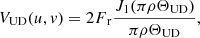
where J1 is the first-order Bessel function;  , where u and v are the spatial frequencies sampled by the interferometric observations; ΘUD is the angular diameter of the UD profile; and Fr is the scaling factor that accounts for the overresolved flux in the observations. To fit the data, we used a Markov chain Monte Carlo (MCMC) algorithm based on the Python package emcee (Foreman-Mackey et al. 2013). We let 250 independent chains evolve for 1000 steps, using the data of each one of the spectral bins independently. Finally, we averaged the best-fit UD diameters. This gave us an estimate of
  = 10.23 ± 0.05 mas (1.86 ± 0.01 au) for the 2014 epoch and
  = 13.77 ± 0.14 mas (2.51 ± 0.23 au) for the 2020 epoch.
3.2. Asymmetries in the stellar disk: Regularized image reconstruction
To characterize the asymmetric structure of R Car observed in the large CP variations, we reconstructed aperture-synthesis images. For the 2014 image, we adopted the methodology outlined by J. Sanchez-Bermudez and detailed in Monnier et al. (2014). Initially, geometrical models were fitted to the interferometric observables, starting with a single component, such as Gaussians or disks. Then, additional components were successively added to minimize the difference between the data and the models through a χ2 minimization process. Once a relatively good approximation to the data was achieved, an image was generated using the best-fit model. This best-fit model was employed as a prior image in BSMEM (Baron & Young 2008). The pixel sampling for the image reconstruction was selected to be 0.3 mas pixel−1, with a pixel grid of 135 × 135 pixels. After the reconstruction process, a χ2 ∼ 6 was achieved. No further adjustments were made to this image setup, as the resulting image had been previously compared with other methods and reconstructions, confirming the validity of the observed structures.
For the 2020 data, we recovered images using a combination of SQUEEZE (Baron et al. 2010) and BSMEM (Baron & Young 2008). We recovered the images using a pixel sampling of 0.3 mas pixel, with a pixel grid of 256 × 256 pixels (which enclosures a field of view of ∼77 mas). First, we ran SQUEEZE using 17 000 iterations over 1000 independent chains. The images were recovered independently at each of the six wavelength channels. Two regularization functions were used: total variation and compactness with hyperparameter values of one and twenty (see Sanchez-Bermudez et al. 2018, for a more complete description of each regularizer). With this setup, we ensured the convergence of most of the chains with χ2 < 4. When comparing the images, we did not find significant differences across spectral channels, so we averaged the chains that converged into a single image. Finally, that mean image was used as a starting point for BSMEM (which uses entropy as a regularizer) to smooth it without increasing the residuals in the model fitting. BSMEM converged in less than 100 iterations. Figure 1 shows our mean best-fit images from the 2014 and 2020 data. Figures C.1 and C.2 show the comparison between the synthetic V2 and CPs, extracted from the two reconstructed images, and the data.
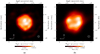 |
Fig. 1. Best-fit reconstructed images for the 2014 (left) and 2020 (right) data sets. The white circles located in the right corner of the images correspond to the maximum resolution of the interferometer. |
3.3. Power spectrum analysis
The H-band images of R Car’s surface shown in Fig. 1 reveal the presence of several large bright spots. Comparison between the two images showed that those features have undergone changes over the course of seven pulsation periods from 2014 to 2020. We performed the analysis of the images’ power spectral density (PSD) to estimate the characteristic size of the structures (Paladini et al. 2018). The first step was to calculate the squared modulus of the Fourier transform of the reconstructed images. The power spectrum of an image shows the flux distribution per spatial scale or spatial frequency. The smallest frequency is the one that encloses all the normalized intensity in the image, and the highest frequency is the one that maps the normalized intensity of the most compact features. To remove the stellar disk contribution from the PSD, we set the images’ pixel values below 70% and 90% of the intensity’s peak (for the 2014 and 2020 epochs, respectively) to the median flux of the pixels above the mentioned threshold values. To characterize the weight of the power, P(k), at a given frequency, k, we computed the momentum of the power spectrum PSD(k) = k × P(k)/Ptot.
In order to estimate the loci of the spatial frequencies that dominate the PSDs, we averaged them radially. Figure 2 shows the resulting radial averaged PSDs for both epochs. We fit a Gaussian to the PSDs’ peaks to determine the dominant spatial frequencies that trace the characteristic sizes of the structures in the surface of our object. For the Gaussian fitting, we used the Python tool lmfit (Newville et al. 2016). Since we only have a single image from the 2014 epoch, the reported uncertainties correspond to the standard deviation of the Gaussian fit. For the 2020 data, the model fitting was performed individually per spectral channel, and the reported errors correspond to the mean of the standard deviation of the best-fit peak positions across the wavelengths. The Gaussian center was limited within the range of −0.6 < log(k) < − 0.2 for the 2014 epoch and −0.7 < log(k) < − 0.3 for the 2020 epoch. The measured maxima in the PSDs trace sizes of 1.82 ± 0.16 mas (4.94 × 10¹⁰ ± 4.89 × 10⁹ m) and 2.51 ± 0.32 mas (6.82 × 10¹⁰ ± 9.59 × 10⁹ m) for the 2014 and 2020 epochs, respectively.
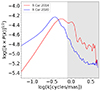 |
Fig. 2. Radial averaged power spectra of the reconstructed images. The red and blue lines show the logarithm of the radial averaged power spectrum versus the logarithm of the spatial frequencies (in cycles mas−1) of the 2014 and 2020 data, respectively. The gray shaded area corresponds to spatial frequencies higher than the best resolution element of the interferometer. |
The derived sizes are bigger than the effective resolution elements of both epochs. However, since the PSD of our images can be affected by the interferometer resolution and the image reconstruction process, we quantified their impact on the determination of the measured sizes of the structures. For that purpose, we simulated two models with the following setups: In the first one, we created two UD spots with a diameter equal to the maximum angular resolution of the interferometer (1.2 mas), and in the second one, we generated two UD spots with a diameter equal to the size of the surface structures derived from the 2020 image (1.8 mas).
We extracted the interferometric observables from these two models using the interferometric u − v coverage from the 2020 epoch. We used this epoch because those data are sparser than the 2014 data. Hence, we expected bigger u − v plane systematics on the reconstructed images. We performed the reconstructions following the same process as the original data. After convolving our images with the resolution of the interferometer and extracting the characteristic (dominant) size of the structures in the images using the PSD analysis, we found that the sizes of the reconstructed spots were quite similar to the original diameters used in the models: 1.30 ± 0.01 mas and 1.81 ± 0.03 mas for the first and second simulated reconstructed images, respectively. The biggest effect was observed in the reconstructed image of the first model, with a difference of Δ ∼ 0.1 mas when the simulated spot diameter is at the maximum resolution of the interferometer. However, when the simulated spot diameter equals the minimum sizes of the measured structures, the size is properly recovered with the PSD analysis. Hence, with those tests, we confirmed that the effect of the interferometer resolution and u − v coverage do not appear to have a significant effect on the sizes of the bright spots on the surface of R Car measured with the used analysis.
4. Discussion
4.1. Sizes of the stellar disk and of the surface structures
The analyzed epochs were obtained on a time baseline larger than the pulsation period of the star and hence are part of different pulsation cycles. However, because of the stable nature of the visual light curve (e.g., no sudden flux drops observed and/or secondary periods), it is reasonable to assume that the star’s properties have not changed fundamentally across the time span between our observations. Thus, throughout rest of the text, we speak in terms of pulsation phase rather than in years of observation.
The PSD analysis showed that the diameter of the star is smaller in phase 0.78, and larger after the photometric maximum at phase 1.01. Ireland et al. (2004) used self-excited pulsation models for M-type Mira stars to make predictions of diameter variations with pulsation for the broad H-band (Hofmann et al. 1998). Those models predict a shift between the size variation and the light curve. The phase shift depends on the band of observation. In the H-band, the object is expected to be smaller around phase 0.8 and larger before the minimum of the pulsation phase. The computed diameters agree with this trend.
It is even more remarkable that the surface patterns change in size between the two pulsation phases. On average, they are smaller when the star is smaller and larger when the star is larger. While this effect is expected from basic physics, to our knowledge, this is the first time that it is shown for the same star using images and with a quantitative analysis such as the PSD. These recovered PIONIER-VLTI images thus open a new dimension in the study of the pulsation of stars. After several years of optical interferometry measuring diameter changes through the pulsation of the AGBs, the time and technology seem mature enough to measure the change in diameter of surface structures throughout the pulsation cycle.
4.2. Convective pattern size(s) and their correlation with the stellar parameters
Paladini et al. (2018) used interferometric observations to compare the structures on the surface of the S-type AGB star π1 Gru with theoretical predictions derived from the mixing-length theory of convection (Ulrich 1970). Those authors used empirical relations of convective cell sizes obtained from 2D and 3D convective models calibrated with solar cell sizes and applied to different stellar types (Freytag et al. 1997; Trampedach et al. 2013; Tremblay et al. 2013). These authors found that the convective structures on the surface of π1 Gru were consistent with the extrapolations of those convection models, suggesting that the convective process could be similar for different stellar types across the H–R diagram.
To uncover the nature of the observed bright structures on the surface of R Car, we conducted the same experiment and compared our measurements described in Sect. 3.3 with the extrapolations of the models used by Paladini et al. (2018). First, according to Freytag et al. (1997; hereafter FR97), the horizontal granulation size, xg, is related to the characteristic pressure scale height, Hp, by the following expression:

where Hp = RgasTeff/μ g, with Teff as the effective temperature of the star, μ as the mean-molecular weight, g as the surface gravity of the star, and Rgas as the ideal gas constant. Equation (2) could be rewritten using the following logarithmic form:

We calculated the predicted convective cell size of R Car using Teff = 2800 K (McDonald et al. 2012), Rgas = 8.314 × 10⁷ erg K−1 mol−1, and μ = 1.3 g mol−1 for a non-ionized solar mixture with 70% hydrogen, 28% helium, and 2% heavier elements (Grevesse & Sauval 1998). To estimate log(g), we used the mass reported in Takeuti et al. (2013) of 0.87 M⊙. Considering the radii derived in Sect. 3.1, we estimated log(g) values of −0.241 and −0.498 for the 2014 and 2020 epochs, respectively2.
Second, Trampedach et al. (2013; hereafter TRA13) defined the following expression to calculate the cell size:
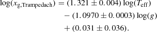
The same Teff and log(g) values used in Eq. (3) are employed in this prescription. Third, using the CIFIST grid, Ludwig et al. (2009) and Tremblay et al. (2013; hereafter TRE13) derived the following equation for xg:
![$$ \begin{aligned} \log (x_{\rm g,Tremblay})&= 1.75\log [T_{\rm eff}-300\log (g)]\nonumber \\&\quad -\log (g) + 0.05[Fe/H] - 1.87. \end{aligned} $$](/articles/aa/full_html/2024/08/aa49112-23/aa49112-23-eq8.gif)
In this formula, we assumed solar metallicity [Fe/H] = 0 and the same values of Teff and log(g) as in TRA13 and FR97. The logarithms of the previously derived values of xg are reported in Table 1. Figure 3 also displays the logarithm of the derived xg for the two reconstructed images as well as the three prescriptions. For comparison, we plotted the value of xg reported by Paladini et al. (2018) for π1Gru.
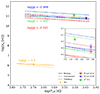 |
Fig. 3. Logarithmic scale of the convective patterns (xg) versus effective temperature (Teff). The different lines correspond to the predictions of convective cell sizes from Freytag et al. (1997), Trampedach et al. (2013), and Tremblay et al. (2013; see the labels on the plot). The blue and red circles correspond to the characteristic scale of the surface structures obtained directly from the reconstructed images of R Car, and the green triangle shows the logarithmic value of xg reported by Paladini et al. (2018) for π1Gru. |
Logarithm of the characteristic size of the patterns observed on the surface R Car.
In angular scales, the xg from the models vary from 1 to 5 mas, which are the lower and upper boundaries set by the TRE13 and TRA13 prescriptions, respectively. The xg derived from our reconstructed images have the sizes 1.82 ± 0.16 mas and 2.51 ± 0.32 mas for the 2014 and 2020 data, respectively, situating them between the boundaries predicted by the models. This would imply a maximum of ∼127 cells existing on the surface of the star if we assume that all structures have a single size and can be considered circular. This is below the limit of 400 cells predicted by Schwarzschild (1975). We find it is important to highlight that the derived sizes are larger than the minimum resolution of our interferometer (1.3 mas), even when including the effects introduced by the image reconstruction process.
Our estimations of the characteristic size of the bright structures on the surface of R Car also follow the predicted pattern from different pulsation phases, as they are smaller when the star is contracted and larger when the star expands. Despite this agreement with the theoretical predictions, recent 3D convection models for AGB stars have suggested that convection acts in a more complex way than the FR97, TRA13, and TRE13 scale relationships suggest (see e.g., Colom i Bernadich 2020). For example, a lower surface gravity implies low densities in both the atmosphere and in the outer layers of the convection zone. This effect leads to large convective velocities, which imply much more violent convection when compared with, for example, the Sun. Moreover, large convective velocities cause large amounts of material to overshoot above the top of the convective-unstable layers. This causes the material to cool down and become optically thick due to molecular opacities. In this case, what could be observed as bright structures on the surface of the star are not the characteristic cell sizes but the material as seen through the gaps created between the elevated, optically thick material.
This effect appears to be more important in more massive objects. For example, Chiavassa et al. (2011) have already suggested that the radiative energy transport in RSGs is more efficient than in the Sun. RSGs are prone to higher pressure fluctuations than AGBs. As a consequence, two kinds of surface structures might appear in those kinds of stars: (i) small-scale short-lived convective features whose sizes are consistent with the models used in Paladini et al. (2018) and in this work but cannot be resolved by the interferometers due to the (on average) more distant location of RSGs (as highlighted by Climent et al. 2020) and (ii) large-scale long-lived features whose sizes are consistent with modified scale relationship predictions in which turbulent motions are included (Norris et al. 2021; Chiavassa et al. 2011).
Nonetheless, the fact that for R Car and π1 Gru the measured bright spot sizes are consistent with the extrapolations from the FR97, TRA13, and TRA13 scale relationships suggests that we are observing the typical convective cell sizes, probably because both AGB stars have similar surface gravities and progenitor masses close to solar. Thus, their convective processes are more similar to those of the Sun, which appears not to be the case for more massive objects.
5. Conclusions
We report the analysis of PIONIER-VLTI interferometric data of the M-type Mira star R Car. Those data consist of archival observations from 2014 and new data obtained in 2020. As a first step, we measured the stellar disk size and its change (ΔR ∼ 0.3R*) at different pulsation phases using parametric model fitting.
The asymmetries observed on the surface of this object were characterized by using image reconstruction and power spectrum analyses. Our findings suggest that the characteristic sizes of these structures are consistent with the extrapolations of three different models of convection. Those models establish convective cell sizes proportional to approximately ten times the pressure scale height in the atmosphere of the target. Our measurements of the convective structures on the surface of R Car support that these structures grow when the stellar disk expands and that they decrease when the star contracts within a pulsation cycle. This work is the first to report this finding for Mira-type AGB stars.
These results add important evidence to the still scarce observational proofs of the role of convection in the evolution of AGB stars. However, state-of-the-art simulations and interferometric observations of more massive objects suggest that convection is more complex. Therefore, the FR97, TRE13, and TRA13 scale relationships differ from predictions for more massive objects and/or when AGB stellar parameters change considerably from the ones tested with R Car.
To better constrain the existing models, future H-band aperture-synthesis (dynamic) images with a time baseline smaller than the pulsation cycle of R Car are thus necessary, with the aim of describing the time evolution of the convective cell patterns and characterizing the living time of such structures. A proper comparison of such observations with hydrodynamic radiative transfer models will be mandatory. Further VLTI observations of additional AGB stars using different infrared bands (from 2.2 to 12 μm) are also part of our current and future efforts to characterize the role of convection and pulsation in shaping the evolution of O-rich Miras.
We note that we also expected a change in temperature as a function of the radius for the two phases. This effect should not be large given that the maximum variability in the H-band is around 0.5 mag (Ireland et al. 2004). However, with the actual data, we could not quantify this change, so we used the same effective temperature for the two data sets.
Acknowledgments
A.R.-G. acknowledges the support received through the Ph.D. scholarship (No. 760678) granted by the Mexican Council of Science CONAHCyT. A.R.-G. acknowledges the support received from the SSDF 2023-5 project “Scanning the atmosphere of R Car” from the European Southern Observatory. J.S.-B. and A.R.-G. acknowledge the support received from the UNAM PAPIIT project IA 105023; and from the CONAHCyT “Ciencia de Frontera” project CF-2019/263975. J.S.-B. acknowledges the support received from the “Science Visitor Programme” from the European Southern Observatory and from the “Fizeau Exchange Programme” funded by WP 17 via OPTICON/RadioNET PIlot Program (grant agreement 101004719). The research leading to these results has received funding from the European Union’s Horizon 2020 research and innovation programme under Grant Agreement 101004719 (ORP). BF and SH acknowledge funding from the European Research Council (ERC) under the European Union’s Horizon 2020 research and innovation programme (Grant agreement No. 883867, project EXWINGS). MM acknowledges funding from the Programme Paris Region fellowship supported by the Région Ile-de-France. This project has received funding from the European Union’s Horizon 2020 research and innovation program under the Marie Skłodowska-Curie Grant agreement No. 945298. RS acknowledges financial support from the State Agency for Research of the Spanish MCIU through the “Center of Excellence Severo Ochoa” award for the Instituto de Astrofísica de Andalucía (SEV-2017-0709), from grant EUR2022-134031 funded by MCIN/AEI/10.13039/501100011033 and by the European Union NextGenerationEU/PRTR, and from grant PID2022-136640NB-C21 funded by MCIN/AEI 10.13039/501100011033 and by the “European Union”. This research has made use of the Jean-Marie Mariotti Center OIFits Explorer service (Available at http://www.jmmc.fr/oifitsexplorer). We acknowledge with thanks the variable star observations from the AAVSO (Available at https://www.aavso.org/) International Database contributed by observers worldwide and used in this research.
References
- Allard, F., Guillot, T., Ludwig, H. G., et al. 2003, Symposium-International Astronomical Union (Cambridge: Cambridge University Press), 211, 325 [CrossRef] [Google Scholar]
- Baron, F., & Young, J. S. 2008, in Optical and Infrared Interferometry, International Society for Optics and Photonics, 7013, 70133X [NASA ADS] [CrossRef] [Google Scholar]
- Baron, F., Monnier, J. D., & Kloppenborg, B. 2010, in Optical and Infrared Interferometry II, International Society for Optics and Photonics, 7734, 77342I [CrossRef] [Google Scholar]
- Bladh, S., & Höfner, S. 2012, A&A, 546, A76 [NASA ADS] [CrossRef] [EDP Sciences] [Google Scholar]
- Brown, A. G., Vallenari, A., Prusti, T., et al. 2021, A&A, 649, A1 [NASA ADS] [CrossRef] [EDP Sciences] [Google Scholar]
- Chiavassa, A., Freytag, B., Masseron, T., & Plez, B. 2011, A&A, 535, A22 [NASA ADS] [CrossRef] [EDP Sciences] [Google Scholar]
- Climent, J., Wittkowski, M., Chiavassa, A., et al. 2020, A&A, 635, A160 [NASA ADS] [CrossRef] [EDP Sciences] [Google Scholar]
- Colom i Bernadich, M. 2020, Measuring the Characteristic Sizes of Convection Structures in AGB Stars with Fourier Decomposition Analyses: the Stellar Intensity Analyzer (SIA) Pipeline [Google Scholar]
- Cox, J. P. 2017, Theory of Stellar Pulsation.(PSA-2), Volume 2 (Princeton: Princeton University Press), 31 [Google Scholar]
- Foreman-Mackey, D., Hogg, D. W., Lang, D., & Goodman, J. 2013, PASP, 125, 306 [Google Scholar]
- Freytag, B., Holweger, H., Steffen, M., & Ludwig, H. G. 1997, Science with the VLT Interferometer: Proceedings of the ESO Workshop Held at Garching, Germany, 18–21 June 1996 (Springer), 316 [CrossRef] [Google Scholar]
- GRAVITY Collaboration (Abuter, R., et al.) 2017, A&A, 602, A94 [NASA ADS] [CrossRef] [EDP Sciences] [Google Scholar]
- Grevesse, N., & Sauval, A. 1998, Space Sci. Rev., 85, 161 [NASA ADS] [CrossRef] [Google Scholar]
- Groenewegen, M., Baas, F., Blommaert, J., et al. 1999, A&AS, 140, 197 [NASA ADS] [CrossRef] [EDP Sciences] [Google Scholar]
- Hanbury Brown, R., Davis, J., & Allen, L. 1974, MNRAS, 167, 121 [NASA ADS] [CrossRef] [Google Scholar]
- Hofmann, K.-H., Scholz, M., & Wood, P. 1998, A&A, 339, 846 [NASA ADS] [Google Scholar]
- Höfner, S., Bladh, S., Aringer, B., & Eriksson, K. 2022, A&A, 657, A109 [NASA ADS] [CrossRef] [EDP Sciences] [Google Scholar]
- Ireland, M., Scholz, M., Tuthill, P. G., & Wood, P. R. 2004, MNRAS, 355, 444 [NASA ADS] [CrossRef] [Google Scholar]
- Kupka, F. 2004, Proc. Int. Astron. Union, 2004, 119 [CrossRef] [Google Scholar]
- Le Bouquin, J. B., Berger, J. P., Lazareff, B., et al. 2011, A&A, 535, A67 [NASA ADS] [CrossRef] [EDP Sciences] [Google Scholar]
- Lebzelter, T., Hinkle, K. H., Wood, P. R., Joyce, R. R., & Fekel, F. C. 2005, A&A, 431, 623 [NASA ADS] [CrossRef] [EDP Sciences] [Google Scholar]
- Ludwig, H. G., Caffau, E., Steffen, M., et al. 2009, Mem. Soc. Astron. It., 80, 711 [Google Scholar]
- McDonald, I., Zijlstra, A. A., & Boyer, M. L. 2012, MNRAS, 427, 343 [Google Scholar]
- Monnier, J. D., Berger, J.-P., Le Bouquin, J.-B., et al. 2014, in Optical and Infrared Interferometry IV, International Society for Optics and Photonics, 9146, 91461Q [NASA ADS] [Google Scholar]
- Newville, M., Stensitzki, T., Allen, D. B., et al. 2016, Astrophysics Source Code Library [record ascl:1606.014] [Google Scholar]
- Norris, R. P., Baron, F. R., Monnier, J. D., et al. 2021, ApJ, 919, 124 [NASA ADS] [CrossRef] [Google Scholar]
- Paladini, C., Baron, F., Jorissen, A., et al. 2018, Nature, 553, 310 [NASA ADS] [CrossRef] [Google Scholar]
- Perrin, G., Ridgway, S. T., Lacour, S., et al. 2020, A&A, 642, A82 [NASA ADS] [CrossRef] [EDP Sciences] [Google Scholar]
- Rosales-Guzmán, A., Sanchez-Bermudez, J., Paladini, C., et al. 2023, A&A, 674, A62 [NASA ADS] [CrossRef] [EDP Sciences] [Google Scholar]
- Samus, N., Kazarovets, E., Durlevich, O., Kireeva, N., & Pastukhova, E. 2017, Astron. Rep., 61, 80 [CrossRef] [Google Scholar]
- Sanchez-Bermudez, J., Millour, F., Baron, F., et al. 2018, Exp. Astron., 46, 457 [NASA ADS] [CrossRef] [Google Scholar]
- Schwarzschild, M. 1975, ApJ, 195, 137 [NASA ADS] [CrossRef] [Google Scholar]
- Takeuti, M., Nakagawa, A., Kurayama, T., & Honma, M. 2013, PASJ, 65, 60 [NASA ADS] [CrossRef] [Google Scholar]
- Trampedach, R., Asplund, M., Collet, R., Nordlund, Å., & Stein, R. F. 2013, ApJ, 769, 18 [NASA ADS] [CrossRef] [Google Scholar]
- Tremblay, P.-E., Ludwig, H.-G., Freytag, B., Steffen, M., & Caffau, E. 2013, A&A, 557, A7 [NASA ADS] [CrossRef] [EDP Sciences] [Google Scholar]
- Ulrich, R. K. 1970, Astrophys. Space Sci., 7, 71 [NASA ADS] [CrossRef] [Google Scholar]
- Whitelock, P. A., Feast, M. W., & Van Leeuwen, F. 2008, MNRAS, 386, 313 [CrossRef] [Google Scholar]
- Wittkowski, M., Hofmann, K.-H., Höfner, S., et al. 2017, A&A, 601, A3 [NASA ADS] [CrossRef] [EDP Sciences] [Google Scholar]
Appendix A: PIONIER observations list
Log of the observations for the 2014 data.
Log of the observations for the 2020 data.
Appendix B: Visual light curve and interferometric u-v coverage
In this section, we present the visual light curve of R Car as a function of the phase and the interferometric u-v coverage of our observed data. Table B.1 displays the different observation epochs from the 2020 data set, which are color coded in the same way as they appear in Fig. B.1. We have included the maximum achievable angular resolution for each configuration as well as the percentage of the total data covered by each epoch. Considering that the reported size of the convective structures is 1.82 ± 0.16 mas and that the highest resolution is achieved with the A0-G1-J2-K0 configuration (1.29 mas), we could conclude that configurations with the largest time interval (A0-B2-C1-D0) map larger structures, such as the stellar disk, while configurations that trace the smaller structures, such as the convective structures, are less temporally spaced. Therefore, we did not expect including this data set in our data to cause a change in the smaller structures.
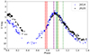 |
Fig. B.1. Visual light curves of R Car obtained from the https://www.aavso.org/ database as a function of the pulsation phase around the dates of our interferometric observations. The blue stars and the black circles correspond to the data of the 2014 and 2020 epochs, respectively. The vertical red-shaded area indicates the phase of the 2014 interferometric observations, while the green, orange, and purple areas correspond to the 2020 ones at different station configurations: short, long, and astrometric, respectively (see Tables A.1 and A.2). |
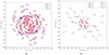 |
Fig. B.2. PIONIER u-v coverages of the data sets used in this study. The left panel corresponds to the 2014 data set, and the right one corresponds to the 2020 one. The colors in the panels show the different wavelengths covered with the bandpass of the instrument (see the labels in the plot). |
Description of our 2020 observations.
Appendix C: Interferometric observables
In this section, we show the comparison between the synthetic and observed V2 and CPs for our 2014 and 2020 epochs (see Sect. 3.2). In both figures, the red dots correspond to the synthetic V2 and CPs extracted from the raw reconstructed images, while the data are shown with gray dots. For a better visualization, the insets show a zoom-in, in logarithmic scale, of the region between 1.5 and 9 × 10⁷ rad−1. The lower panels show the residuals (in terms of the number of standard deviations) coming from the comparison between the data and the best-reconstructed images.
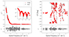 |
Fig. C.1. Fit to the observed V2 (left panel) and CPs (right panel) from the 2014 mean reconstructed image as a function of the spatial frequency. |
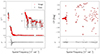 |
Fig. C.2. Fit to the observed V2 (left panel) and CPs (right panel) from the 2020 mean reconstructed image as a function of the spatial frequency. |
All Tables
Logarithm of the characteristic size of the patterns observed on the surface R Car.
All Figures
|
Fig. 1. Best-fit reconstructed images for the 2014 (left) and 2020 (right) data sets. The white circles located in the right corner of the images correspond to the maximum resolution of the interferometer. |
| In the text | |
|
Fig. 2. Radial averaged power spectra of the reconstructed images. The red and blue lines show the logarithm of the radial averaged power spectrum versus the logarithm of the spatial frequencies (in cycles mas−1) of the 2014 and 2020 data, respectively. The gray shaded area corresponds to spatial frequencies higher than the best resolution element of the interferometer. |
| In the text | |
|
Fig. 3. Logarithmic scale of the convective patterns (xg) versus effective temperature (Teff). The different lines correspond to the predictions of convective cell sizes from Freytag et al. (1997), Trampedach et al. (2013), and Tremblay et al. (2013; see the labels on the plot). The blue and red circles correspond to the characteristic scale of the surface structures obtained directly from the reconstructed images of R Car, and the green triangle shows the logarithmic value of xg reported by Paladini et al. (2018) for π1Gru. |
| In the text | |
|
Fig. B.1. Visual light curves of R Car obtained from the https://www.aavso.org/ database as a function of the pulsation phase around the dates of our interferometric observations. The blue stars and the black circles correspond to the data of the 2014 and 2020 epochs, respectively. The vertical red-shaded area indicates the phase of the 2014 interferometric observations, while the green, orange, and purple areas correspond to the 2020 ones at different station configurations: short, long, and astrometric, respectively (see Tables A.1 and A.2). |
| In the text | |
|
Fig. B.2. PIONIER u-v coverages of the data sets used in this study. The left panel corresponds to the 2014 data set, and the right one corresponds to the 2020 one. The colors in the panels show the different wavelengths covered with the bandpass of the instrument (see the labels in the plot). |
| In the text | |
|
Fig. C.1. Fit to the observed V2 (left panel) and CPs (right panel) from the 2014 mean reconstructed image as a function of the spatial frequency. |
| In the text | |
|
Fig. C.2. Fit to the observed V2 (left panel) and CPs (right panel) from the 2020 mean reconstructed image as a function of the spatial frequency. |
| In the text | |
Current usage metrics show cumulative count of Article Views (full-text article views including HTML views, PDF and ePub downloads, according to the available data) and Abstracts Views on Vision4Press platform.
Data correspond to usage on the plateform after 2015. The current usage metrics is available 48-96 hours after online publication and is updated daily on week days.
Initial download of the metrics may take a while.