| Issue |
A&A
Volume 687, July 2024
|
|
|---|---|---|
| Article Number | A72 | |
| Number of page(s) | 13 | |
| Section | Catalogs and data | |
| DOI | https://doi.org/10.1051/0004-6361/202449831 | |
| Published online | 01 July 2024 | |
The solar cycle 25 multi-spacecraft solar energetic particle event catalog of the SERPENTINE project★
1
Department of Physics and Astronomy, University of Turku,
Finland
e-mail: This email address is being protected from spambots. You need JavaScript enabled to view it.
2
Department of Physics, University of Helsinki,
PO Box 64,
00014
Helsinki,
Finland
3
Institute of Experimental and Applied Physics, Kiel University,
Kiel,
Germany
4
Universidad de Alcalá, Department of Physics, Space Research Group,
Alcalá de Henares,
Spain
5
Leibniz-Institut für Astrophysik Potsdam (AIP),
An der Sternwarte 16,
14482
Potsdam,
Germany
6
The Blackett Laboratory, Department of Physics, Imperial College London,
London
SW7 2AZ,
UK
7
Fachhochschule Nordwestschweiz,
Bahnhofstrasse 6,
5210
Windisch,
Switzerland
8
ETH Zürich,
Rämistrasse 101,
8092
Zürich,
Switzerland
9
European Space Agency, ESTEC,
Keplerlaan 1,
2201 AZ
Noordwijk,
The Netherlands
10
NASA Goddard Space Flight Center,
Greenbelt,
MD
20771,
USA
11
California Institute of Technology,
Pasadena,
CA
91125,
USA
12
Johns Hopkins University Applied Physics Laboratory,
Laurel,
MD
20723,
USA
Received:
1
March
2024
Accepted:
19
April
2024
Abstract
Context. The solar energetic particle analysis platform for the inner heliosphere (SERPENTINE) project, funded through the H2020-SPACE-2020 call of the European Union’s Horizon 2020 framework program, employs measurements of the new inner heliospheric spacecraft fleet to address several outstanding questions on the origin of solar energetic particle (SEP) events. The data products of SERPENTINE include event catalogs, which are provided to the scientific community.
Aims. In this paper, we present SERPENTINE’s new multi-spacecraft SEP event catalog for events observed in solar cycle 25. Observations from five different viewpoints are utilized, provided by Solar Orbiter, Parker Solar Probe, STEREO A, BepiColombo, and the near-Earth spacecraft Wind and SOHO. The catalog contains key SEP parameters for 25–40 MeV protons, ~1 MeV electrons, and ~100 keV electrons. Furthermore, basic parameters of associated flares and type II radio bursts are listed, as are the coordinates of the observer and solar source locations.
Methods. An event is included in the catalog if at least two spacecraft detect a significant proton event with energies of 25–40 MeV. The SEP onset times were determined using the Poisson-CUSUM method. The SEP peak times and intensities refer to the global intensity maximum. If different viewing directions are available, we used the one with the earliest onset for the onset determination and the one with the highest peak intensity for the peak identification. We furthermore aimed to use a high time resolution to provide the most accurate event times. Therefore, we opted to use a 1-min time resolution, and more time averaging of the SEP intensity data was only applied if necessary to determine clean event onsets and peaks. Associated flares were identified using observations from near Earth and Solar Orbiter. Associated type II radio bursts were determined from ground-based observations in the metric frequency range and from spacecraft observations in the decametric range.
Results. The current version of the catalog contains 45 multi-spacecraft events observed in the period from November 2020 until May 2023, of which 13 events were found to be widespread (observed at longitudes separated by at least 80° from the associated flare location) and four could be classified as narrow-spread events (not observed at longitudes separated by at least 80° from the associated flare location). Using X-ray observations by GOES/XRS and Solar Orbiter/STIX, we were able to identify the associated flare in all but four events. Using ground-based and space-borne radio observations, we found an associated type II radio burst for 40 events. In total, the catalog contains 142 single event observations, of which 20 (45) have been observed at radial distances below 0.6 AU (0.8 AU). It is anticipated that the catalog will be extended in the future.
Key words: Sun: flares / Sun: heliosphere / Sun: particle emission / solar-terrestrial relations
Available at https://doi.org/10.5281/zenodo.10732268
© The Authors 2024
 Open Access article, published by EDP Sciences, under the terms of the Creative Commons Attribution License (https://creativecommons.org/licenses/by/4.0), which permits unrestricted use, distribution, and reproduction in any medium, provided the original work is properly cited.
This article is published in open access under the Subscribe to Open model. This email address is being protected from spambots. You need JavaScript enabled to view it. to support open access publication.
1 Introduction
Solar energetic particle (SEP) events are large outbursts of energetic particle radiation from the Sun associated with solar eruptions; that is, solar flares and coronal mass ejections (CMEs). They can be classified based on their key observational properties; for example, in impulsive and gradual classes (e.g., Reames 1999). The classical picture relates impulsive events with flares and gradual events with fast and wide CMEs. While the broad lines of the origin of SEP events are mostly understood, many of the key aspects of the acceleration and transport of ions and electrons in these events have remained elusive. The main obstacle preventing us from achieving a complete understanding has been the lack of observational coverage in the heliosphere: solar eruptions often fill a major part of the inner heliosphere with energetic particles, and using a scarce set of observing spacecraft (S/C) does not allow one to conclusively separate the effects of particle transport from the properties of the source.
With the launch of the new space missions Solar Orbiter (Müller et al. 2020) and Parker Solar Probe (Parker; Fox et al. 2016), a unique era for multi-S/C observations of SEP events has begun. Combined with established space missions near Earth, such as the SOlar and Heliospheric Observatory (SOHO; Domingo et al. 1995) and Wind (Ogilvie & Desch 1997), the Ahead S/C of the Solar Terrestrial Relations Observatory (STEREO A; Kaiser et al. 2008), and the BepiColombo mission on its cruise to Mercury (Benkhoff et al. 2021), these S/C form an unprecedented fleet during the rising phase of solar cycle 25. The various orbits of the missions provide ever-changing S/C constellations covering different heliocentric distances and heliolongitudes. Some SEP events are observed over wide longitudinal ranges in the inner heliosphere (e.g., Kollhoff et al. 2021; Dresing et al. 2023); others by a fleet of closely spaced observers, allowing the study of local effects (e.g., Lario et al. 2022; Palmerio et al. 2024). Sometimes different S/C are radially aligned, permitting one to study radial dependencies, especially during interplanetary CME (ICME) and interplanetary (IP) shock crossings (e.g., Kilpua et al. 2021; Trotta et al. 2023c, 2024). Other events are observed by magnetically aligned S/C; that is, when they are nearly situated on the same Parker spiral magnetic field, connecting them to the same region of the Sun (e.g., Rodríguez-García et al. 2023b; Kollhoff et al. 2023). Such constellations are ideal to investigate radial effects of the parallel transport of SEPs along the same magnetic field line. Inner heliospheric observations can be complemented by SEP measurements at farther distances, such as Mars (e.g., Palmerio et al. 2022; Guo et al. 2023); for example, detection on the surface (Hassler et al. 2012) and in orbit by the MAVEN S/C (Jakosky et al. 2015).
This powerful S/C fleet opens up new opportunities to answer many outstanding questions on the generation of SEP events. One such question is why widespread SEP events show SEP distributions up to all around the Sun, as has been recorded by S/C located at various longitudes. Other questions include how SEPs of different species and energies are accelerated, what the relative roles of associated flares and CME-driven shocks are in particle acceleration and spatial SEP distribution, and what the role is of particle transport in spreading the particles over wide longitudinal regions.
The new knowledge generated with these unprecedented observations will not only further our understanding of the fundamental processes, dominating several astrophysical systems, but eventually lead to better forecasting abilities of space-weather-relevant SEP events at Earth or elsewhere in the Solar System.
This paper describes the building and content of a multi-S/C SEP event catalog of SEP events detected in solar cycle 25 by inner heliospheric space missions; that is, Solar Orbiter, Parker Solar Probe, STEREO A, BepiColombo, and the near-Earth S/C Wind and SOHO. The presented catalog was compiled within the scope of the solar energetic particle analysis platform for the inner heliosphere (SERPENTINE1) project, which is funded through the European Union’s Horizon 2020 framework program under the H2020-SPACE-2020 call topic addressing “Scientific data exploitation”.
The main objective of SERPENTINE is to uncover the primary causes of large, gradual, and widespread SEP events; that is, the respective role of the broad sources and efficient cross-field particle transport in their genesis. The project tackles the challenge through comprehensive analyses, both case studies and statistical investigations, of historical and current SEP measurements and solar context observations (Kollhoff et al. 2021; Dresing et al. 2022, 2023; Rodríguez-García et al. 2023a,b; Wijsen et al. 2023; Jebaraj et al. 2023b,a; Trotta et al. 2022a; Dimmock et al. 2023; Lorfing et al. 2023; Kilpua et al. 2023; Trotta et al. 2023c,b,a, 2024). One of the most important outcomes of the project is the public release of data analysis tools (Kouloumvakos et al. 2022; Palmroos et al. 2022; Price et al. 2022; Trotta et al. 2022b; Gieseler et al. 2023; Kouloumvakos et al. 2023) and catalogs of SEP events, IP shocks, and CMEs for historical and solar cycle 25 events. The tools and catalogs were built for easy access and are released in the hope of broad use by the heliophysics community. Altogether, five catalogs, two based on Helios data and three based on modern observations, have been released through the project data server2. Additionally, the presented SEP catalog is accessible and citable as Dresing et al. (2024) through Zenodo3.
This paper presents the SERPENTINE catalog of the SEP events of solar cycle 25 to date. The catalog focuses on energetic SEP events, those producing at least 25 MeV protons, which are potentially relevant for space weather, and aims to provide a comprehensive resource to exploit the novel multi-S/C observations of solar cycle 25.
The paper is organized as follows. In Sect. 2, we introduce the data and energetic particle instruments used; in Sect. 3, we explain the selection criteria for listed events; and in Sect. 4 we present the contents of the catalog and how the parameters were determined. Section 5 presents the results, and Sect. 6 summarizes the work.
2 Data and instrumentation
We utilize energetic particle measurements taken by six space missions: Solar Orbiter, Parker, STEREO A, Wind, SOHO, and BepiColombo. In order to cover the three different SEP energy-species combinations of the catalog, >25-MeV protons as well as ~ 100-keV and ~ 1 -MeV electrons, we use the following instruments: the Energetic Particle Detector (EPD; Rodríguez-Pacheco et al. 2020) instrument suite of Solar Orbiter, the Integrated Science Investigation of the Sun (IS⊙IS; McComas et al. 2016) suite of Parker, the Solar Electron Proton Telescope (SEPT; Müller-Mellin et al. 2008) and the High Energy Telescope (HET, von Rosenvinge et al. 2008) of the STEREO mission, the Three-Dimensional Plasma and Energetic Particle Investigation (3DP; Lin et al. 1995) of the Wind S/C, the Energetic and Relativis-tic Nuclei and Electron (ERNE; Torsti et al. 1995) experiment, and the Electron Proton Helium Instrument (EPHIN), which is part of the Comprehensive Suprathermal and Energetic Particle Analyser (COSTEP; Müller-Mellin et al. 1995) suite of SOHO, as well as the Solar Intensity X-Ray and Particle Spectrometer (SIXS; Huovelin et al. 2020) on board BepiColombo’s Mercury Planetary Orbiter (MPO).
For each of the three energy-species combinations, we aim to provide the SEP parameters at the same energy range as that observed by the different S/C. Because of the different instrumentation on board the various S/C, no perfect overlap is possible. Table 1 summarizes the chosen S/C and instruments (column 1), the energy channels and corresponding mean energies (E) (Cols. 3–5) that were used in the catalog, and the available viewing directions of the instruments (Col. 2). We note that the data product of Parker/EPI-Lo changed in June 2021, which led to a changed energy range and different energy channels being used. In the case of BepiColombo/SIXS, only effective energies of the channels can be determined because of the complex instrument response functions. The energy-range limits provided for BepiColombo/SIXS in Cols. 2 and 4 of Table 1 therefore represent the effective mean energies of the used energy channels. This means that the actual energy channels are significantly wider. For SOHO/EPHIN, it should be noted that the instrument was switched to failure modes D and E in 2017, which excluded the two deepest detectors from any coincidence logic. This resulted in a significant widening of the electron channel E1300. Therefore, the effective mean energy has a strong spectral dependence. The corresponding value of 1.47 MeV shown in Table 1 has been calculated for a spectral index of −24. This corresponds to the average slope of the events considered in this paper (see Sect. 4.4).
Near-relativistic electron measurements employed in our catalog, like the ~100-keV electron channel, are typically realized through a single-detector measurement and the magnet-foil principle, whereby a foil is used to stop protons and ions from reaching the detector. However, ions that penetrate the foil can contaminate the electron measurements, especially during periods when ion fluxes are large compared to the electron fluxes (e.g., Wraase et al. 2018). This is more often the case during SEP peak phases than during SEP onsets due to the usually earlier arrival times of electrons. Therefore, we checked all ~100-keV electron peaks by comparing the electron-intensity time series with those of ions in the contaminating energy ranges and excluded the peaks from the catalog if in doubt.
Key parameters of the associated flare rely on GOES X-ray observations provided by SolarMonitor5. The presence of metric type II radio bursts was also investigated using event lists provided by the Space Weather Prediction Center (SWPC)6. The SWPC collects reports from contributing stations on the ground that provide 24-h coverage. These stations are the Culgoora spectrograph, Learmonth spectrograph, Holloman Solar Observatory, and San Vito Solar Observatory, and they form the Radio Solar Telescope Network (RSTN).
3 Selection criteria
Following previous SEP event catalogs (e.g., Richardson & Cane 2010; Richardson et al. 2014), we based our event selection on energetic proton events observed in the energy range of ~25–40 MeV (see Table 1, column 3). An event was identified based on a visual inspection of 1-h averaged data, requiring a significant increase above the background. Aiming for a multi-S/C catalog, we then selected an event if it was observed by at least two different S/C. Due to the constantly changing S/C constellations, this includes both events observed over wide longitudinal regions (widespread events, cf. Fig. 1) and those observed in only a narrow longitudinal sector (cf. Fig. 2). The latter also includes S/C constellations with radial alignments or those where different S/C are magnetically aligned; that is, where they are situated along the same nominal Parker spiral connecting to the Sun (cf. BepiColombo and STEREO A in Fig. 2). Therefore, one column of the catalog provides cases of potential scientific interest based on the multi-S/C constellation of the observing S/C. Among these science cases are “widespread” and “narrow-spread” events. A widespread event is defined as an event observed by at least one observer with a longitudinal separation, Φ, between the observer’s magnetic footpoint and a flare longitude of ≥80 degrees, following Dresing et al. (2014). Analogously, we call an event a “narrow-spread event” if it is not observed by an observer who has a longitudinal separation angle of Φ ≤ 80 degrees. We note that the ability to identify these wide and narrow particle spreads depends on the specific S/C constellation. Therefore, more wide-or narrow-spread events might be in the sample.
The multi-S/C SEP events were identified based on the observations of temporal coincident enhancements of energetic particle fluxes at the different S/C. Key information about the associated flare is also listed when a flare was reported in the Earth’s or Solar Orbiter’s visible hemisphere.
4 Contents of the catalog and parameter determination
The current version of the catalog is archived and citable as Dresing et al. (2024) through Zenodo,7 where newer versions will be added after every update. The latest version of the catalog can also be accessed via the SERPENTINE data center8 along with (and linked to) further data products and catalogs provided by the SERPENTINE project. In addition to downloading the catalog from the data center, the platform provides various filtering options. Figure 3 shows a screenshot of the catalog’s starting page, which contains only a selection of parameters for each event. After clicking an event ID, a detailed event page opens (see Fig. 4) that presents all event parameters as well as a plot showing the S/C constellation and their nominal magnetic connections with the Sun determined by the Solar-MACH tool (Gieseler et al. 2023). For those events for which an associated flare was identified (see details below), its position was added as a reference (arrow) to the Solar-MACH plot. We note that the Solar-MACH tool provides further coordinate information such as the locations of the S/C magnetic footpoints estimated via ballistic backmapping (using the measured solar wind speed or assuming a solar wind speed of 400 km s−1) as well as the longitudinal separation angles with the flare location. Those values can be retrieved from the Solar-MACH webpage9, when clicking the link below the plot on the catalog page. We note that the SERPENTINE project provides further Python-based tools on the SERPENTINE Hub10, which can be used to perform more in-depth analyses of SEP events. These include tools to load and visualize various SEP measurements as well as a magnetic connectivity tool combining ballistic backmapping with magnetic field extrapolations in the lower corona based on a potential field source surface (PFSS) model (see also, Gieseler et al. 2023; Palmroos et al. 2022).
For each SEP event, the catalog provides various SEP parameters obtained by the five different observer locations as well as flares based on GOES and Solar Orbiter observations, and the presence of type II radio bursts along with their occurrence time and frequency range. The columns of the catalog for each SEP event are as follows:
Event ID: Unique identifier of each SEP event used for linking different SERPENTINE catalogs.
Science case: For example: “widespread event,” “narrow-spread event,” “magnetic alignment of STEREO A and L1,” “radial alignment of BepiColombo and L1.”
Event start date: Date of the associated flare or earliest SEP onset (in case no flare observations are available).
Flare time11 (UT)
Flare latitude12 (º)
Flare longitude12 (º)
Flare class (GOES or GOES equivalent13)
Flare comments
Radio type II burst: Observer names14 are provided in the case of a type II observation, but otherwise left empty.
Decametric radio type II burst start time (UT)
Decametric radio type II burst stop time (UT)
Frequency range of decametric type II burst (MHz)
Metric radio type II burst start time (UT)
Metric radio type II burst stop time (UT)
Frequency range of metric type II burst (MHz)
Metric radio imaging available (yes/no)
Radio comments15
ID of associated CMEs16
-
Solar-MACH link: Link to an S/C constellation plot of the event17
The following columns are provided for each S/C:
S/C latitude12 (º)
S/C longitude12 (º)
S/C radial distance from the Sun (au)
-
ID of associated IP shocks18.
The following columns are provided for each of the three particle species or energy combinations, (i) >25-MeV protons, (ii) ~100-keV electrons, and (iii) ~1-MeV electrons:
- (a)
Onset date: Date of the energetic particle onset at the S/C
- (b)
Onset time: Time of the energetic particle onset at the S/C (UT)
- (c)
Time averaging used for the onset determination (min)
- (d)
Sector used for onset determination: This applies only to those instruments that provide directional energetic particle measurements (see Table 1)
- (e)
Peak date: Date of maximum intensity (UT)
- (f)
Peak time: Time of maximum intensity (UT)
- (g)
Peak flux: Maximum intensity ((s cm2 sr MeV)−1) of the event in the selected energy channel
- (h)
Averaging used for peak determination (min)
- (i)
Sector used for peak determination: Same as (d) (see above)
- (j)
Inferred injection date (UT)
- (k)
Inferred injection time (UT)19, based on the onset time of the selected species and energy channel considering the distance of the S/C and assuming a nominal Parker spiral (see more detail in Sect. 4.3)
- (l)
Path length (au) used for inferred injection time: Length of the nominal Parker spiral considering the distance of the S/C and using the measured solar wind speed
- (m)
Solar wind speed (km s−1) used to determine path length20
- (n)
Event comments21.
- (a)
Electron-proton ratio
Energetic particle instruments, their available viewing directions, and energy channels used for the catalog.
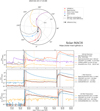 |
Fig. 1 Multi-S/C events of February 24 and 25, 2023. The top plot presents the longitudinal configuration of S/C in the heliographic equatorial plane with respect to the longitude of the associated flare (black arrow) for the event starting on 24 February. The plot was produced with the Solar-MACH tool (Gieseler et al. 2023). The colored spirals denote the magnetic field lines connecting each observer with the Sun. The dashed black spiral represents the field line connecting with the flare. The bottom plot shows the intensity time series of ~100-keV electrons (top), ~1-MeV electrons (middle), and >25-MeV protons (bottom). Parker did not observe the events but a previous event happening earlier on 24 February. Since there is no obvious electron foreground in the EPI-Lo electron measurements (top panel) during the second event, the counts during this time period are background, assumed to be primarily caused by galactic cosmic rays. Parker/HET data were not available during the shown time period. The black arrow on top of the upper panel denotes the times of the associated flares. Solid (dotted) lines mark the onset (peak) times, with colors corresponding to those of the S/C time series. |
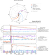 |
Fig. 2 Figure structure as in Fig. 1, but for the event of March 28, 2022. This event was only observed by STEREO A and near-Earth S/C (Wind and SOHO), but not at Solar Orbiter or Parker (BepiColombo/SIXS data were not available). The science case of this event is a “narrow-spread event.” |
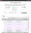 |
Fig. 3 Starting page of the multi-S/C SEP event catalog at the SERPENTINE data center. Various filtering options can be applied by the user. Below, the resulting list of events, including several of the main event parameters, is shown. |
4.1 Flare identification
Several sources were employed to find the most appropriate solar flare that could have produced the observed multi-S/C event. The majority of associated flares were found with the help of SolarMonitor, based on observations of the X-ray sensor (XRS) on board the GOES S/C covering the visible hemisphere of Earth. We also used other resources if no flare candidate was listed at SolarMonitor, which is the catalog of flares observed by the Hinode satellite (Watanabe et al. 2012)22 and the Space Weather Prediction Center.23 If the flare was not visible from Earth’s viewpoint we used flare observations by Solar Orbiter’s X-ray telescope STIX (Krucker et al. 2020) that are provided in the Solar Orbiter flare catalog24. Potentially corresponding flares were identified based on timing coincidence. As a first step, we looked for flares within a time window several hours before the first particle onset until this first onset. Afterward, the flare candidate was corroborated by its location with respect to the S/C constellation, assuming that the magnetically best connected would observe the highest SEP intensities and earliest onset times. If there were several flares that could serve as a potential source, from the point of view of their location, preference was given to the most powerful one and the one which was temporally the closest associated with the first observed SEP onset. For each flare, the catalog records the time of the flare, its Carrington longitude and latitude, and the GOES class, which is based on the X-ray observations. In cases of flares for which Solar Orbiter was viewing the backside of the Sun (i.e., flares not observed with GOES), an estimated GOES class is given based on the counts in the STIX 4–10 keV channel. This estimate is based upon a statistical correlation between the GOES 1–8 Å flux and the STIX 4–10 keV channel for flares observed by both for all events from January 2021 to November 2023 (see Xiao et al. 2023, for further details). We note, however, that this temporal association does not exclude other potential flares in longitudinal sectors not observed with X-ray telescopes that could have contributed to the multi-S/C SEP observations. The user is therefore advised to take this possibility into account and if necessary to analyze the events in more detail themselves.
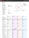 |
Fig. 4 Detailed view of a selected event at the SERPENTINE data center. This page shows all parameters of the selected event. |
4.2 Type II radio burst identification
For each event in the SEP event catalog, the presence of metric and decametric type II radio bursts was investigated. To identify IP type II bursts in the decametric range, we visually inspected daily radio spectrograms25 of Parker Solar Probe, STEREO A, Solar Orbiter, and Wind, and listed which S/C observed the type II. For the metric type II bursts, we used event lists provided by SWPC. In rare cases in which a type II burst was not present in the SWPC lists, we identified the burst from the eCALLISTO event lists26 that are used for confirmation. These lists contain information on solar eruptions, including the presence of radio burst types and their properties obtained from dynamic spectra from the ground-based RSTN telescope network. We extracted only type II radio bursts as these are signatures of shock-accelerated electron beams at the Sun (e.g., Nelson & Melrose 1985; Jebaraj et al. 2020, 2021; Kouloumvakos et al. 2021; Morosan et al. 2019, 2023) and can be used to indicate the presence of a coronal shock, which is relevant for SEP events.
Corresponding bursts were identified based on a temporal association with the flare start time. We only considered those type II bursts that occurred at most 1 h from the flare start time. For both metric and decametric type II bursts we provide timing and frequency information. In the case of the decamet-ric type II burst, we used the S/C that observed the brightest type II burst. In the case of the metric type II bursts, the parameters were extracted from the SWPC event lists. Following the identification of type II bursts associated with SEP events, we also investigated the availability of radio imaging with the Low Frequency Array (LOFAR; van Haarlem et al. 2013) and the Nançay Radioheliograph (NRH; Kerdraon & Delouis 1997). The availability of radio imaging and the imaging instrument are provided in the column of the radio comments.
4.3 Determination of solar energetic particle parameters
The SEP onset times were determined with the Poisson-CUSUM method (Huttunen-Heikinmaa et al. 2005) using the SEP analysis tools of the SERPENTINE project (Palmroos et al. 2022). Figure 1 shows an example of two consecutive SEP events observed on February 24 and 25, 2023. The top plot shows the longitudinal configuration of the S/C fleet with respect to the associated flare (called the “reference longitude”) for the first of the two SEP events. The bottom plot shows the intensity time series of the three energy–species combinations of the catalog: ~100 keV electrons (top), ~1-MeV electrons (middle), and >25 MeV protons (bottom). Onset and peak times are marked by solid and dotted lines, respectively, with the color coding according to the different S/C. We define the event’s peak as the global intensity maximum, which can in some cases be strongly delayed with respect to the onset time. For each onset and peak time the catalog provides the time resolution that was used to determine these parameters. We aim to use 1-min averages for the onset determination if the onset is well defined. For the peak time and peak intensity, we used at least a time averaging of 10 min. However, if the onset determination required more time averaging – that is, more than 10 min – we used at least the same averaging as the one applied for the peak determination.
If the instrument used provided different viewing directions (cf. Table 1), we used the viewing direction that observed the earliest onset time for the onset determination and that had the highest maximum intensity for the peak determination. The respective viewing directions employed are also provided in the catalog.
In case of late intensity maxima, which could be associated with IP shock acceleration, the 100-keV electron measurements can suffer from contamination by ions, which can dominate during later phases of SEP events. In those cases we excluded the 100-keV-electron peak times and intensities. This information is also marked in the respective comments columns.
Although the first event in Fig. 1 was observed by four observers (L1, STEREO A, Solar Orbiter, and BepiColombo), it was not classified as a widespread event because none of the observers’ magnetic footpoints at the Sun has a longitudinal separation with the flare greater than 80 degrees, which would prove a wide SEP spread.
In cases in which an event was not observed by a certain S/C, the catalog still provides the coordinates of the observer location. The value in the peak intensity column then corresponds to the background intensity observed by the respective S/C during the time of the event observed by other S/C, but no peak time is pro-vided27. This allows the user to estimate if the S/C was situated in an environment with increased SEP background levels. An S/C that did not observe an event also serves as an upper limit for the longitudinal extent of the SEP event. Figure 2, for example, shows a narrow-spread event constrained by Solar Orbiter, which did not detect the event.
For each of the three energy species combinations we also provide an inferred solar injection time based on a simple time-shift analysis (e.g., Paassilta et al. 2018) assuming a particle energy corresponding to the mean energy of the used energy channels. Therefore, the onset time is shifted back in time based on the expected travel time of the particles based on their speeds and an assumed path length along a nominal Parker spiral field line. To determine the length of the Parker spiral, we used a 1-h average of the measured solar wind speed at the onset time of the event. If no solar wind speed measurement was available, a speed of 400 km s–1 was used. These measured solar wind speeds are provided in the catalog for each of the three particle types, as their onset times might be different.
4.4 Determination of electron to proton ratios
The catalog contains the electron-to-proton intensity ratio of ~1-MeV electrons and 25–40 MeV protons. The instruments, energy channels, and corresponding mean energies used to determine the electron-to-proton ratios are summarized in Table 2. if not stated otherwise, the mean energies were calculated using a geometric mean of the energy range limits. For the protons, we used the peak intensities that are directly provided in the catalog. The mean energies of the used energy channels provided by the different instruments are very similar, at ~32 MeV. For electrons, we tried to match an energy of ~l MeV as best as possible. This required, however, a more complex utilization of instrument data products, which is described in the following. In the case of STEREO/HET, we used channel 0, which has a geometric mean energy of 0.99 MeV. For SolO/EPD, the energy of 0.99 MeV is situated between the energy ranges covered by the EPT and HET instruments. We therefore used both telescopes and determined the ~ 1-MeV peak intensity using an interpolation between peak intensities determined for channel 1 of HET (1.053–2.401 MeV) and the combined channel 31–33 for EPT (0.37–0.47 MeV), assuming a power law. In those cases in which the event was not observed in the HET energy channel, we extrapolated the EPT peak intensity using an average slope determined from 26 events, where this was possible. The average slope and its standard deviation are −4.87 ± 1.72.
In the case of SOHO/EPHIN, we made use of a new data product. While the previously used level2 data product relied on detector combinations with only a limited energy resolution for electrons, the other extreme was the oft-used so-called pulse height analysis (PHA) data, which provides detailed energy losses in each detector for only a statistical sample of measured particles. Here, we use neither of those but rather the onboard histogram data, which provides a good compromise between counting statistics and energy resolution. Utilizing the bow-tie method (e.g., Raukunen et al. 2020), we were able to derive several energy channels based on this dataset in the energy range between 0.15 MeV to about 1.1 MeV. In this work we make use of two of those new energy channels, E5 (0.45–0.5 MeV) and E15 (0.7–1.1 MeV). The effective mean energy of the E15 channel is 0.955 MeV. To match the desired 0.99 MeV even better, we interpolated between the two intensity values, assuming a spectral slope of a power law just like for the Solar Orbiter measurements (see above). Because we require the intensity peaks in both energy channels to occur within two neighboring time steps based on the used time resolution, some events did not qualify for the interpolation method. In those cases, we corrected the peak intensity of E15, assuming a power law with a spectral slope that had been determined from the 17 events in which the interpolation method could be applied. The average slope used and its standard deviation are −2.46 ± 0.46.
For BepiColombo we used the electron channel 5, which has a nominal mean energy of 0.96 MeV. We note that no exact energy ranges can be provided for BepiColombo/SIXS due to the complex response functions of the instrument. The mean energy provided in Table 2 was determined using a bow-tie analysis with a simulated instrument response function (Huovelin et al. 2020).
Energetic particle instruments, energy channels, and corresponding mean energies used to determine the electron-to-proton ratios.
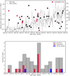 |
Fig. 5 Top: highest > 25 MeV-proton peak intensity observed (black dots) in each event as a function of time, with widespread events marked in red. Daily and monthly sunspot numbers are shown by gray curves (right axis) provided by WDC-SILSO, Royal Observatory of Belgium, Brussels. Bottom: histogram of event occurrences, with all events in gray, widespread events in red, and narrow-spread events in blue. |
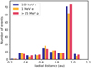 |
Fig. 6 Histogram of S/C distances during event observations for the three different energy-species combinations. |
5 Results
The current version of the catalog contains 45 events covering the period from November 2020 to May 2023. The histogram shown in Fig. 5 (bottom) shows the number of events over time and indicates when widespread and narrow-spread events were observed. The top plot of Fig. 5 shows the highest proton peak intensity observed in each event as a function of time, marking all widespread events in red. We neither observe a clear correspondence between the highest peak intensities and sunspot numbers (also shown in the plot) nor between peak intensities and the occurrence of widespread events. However, we note that our ability to detect a widespread event, or even a narrow-spread one, strongly depends on the available S/C constellation during an event. Therefore, several more of the black points in Fig. 5 (top) could also be widespread events. Furthermore, some of those could even be narrow-spread events as some events occurred during periods when all S/C were located within a narrow longitudinal sector.
Counting all single S/C SEP event observations of the current version of the catalog yields 142 events in total. Counting each energy-species combination separately, we get 414 events for which the catalog provides key parameters. Figure 6 shows the radial distances at which the S/C observed these events. The slight differences in the event numbers based on the different energy-species combinations can be caused by a few events being observed only at lower energies but not extending to higher energies, or by data gaps. With Parker, Solar Orbiter, and BepiColombo, events were also observed at smaller heliocentric distances, with 20 (45) single-S/C events at radial distances below 0.6 AU (0.8 AU).
Figure 7 (top) shows a histogram of the longitudinal separation angles between S/C magnetic footpoints at the Sun and the flare location of all S/C for all events in the catalog, even if no associated SEP event was observed. The three panels below show the longitudinal separation angles only for those observers who detected a ~100-keV electron, ~1-MeV electron, or >25-MeV proton event. These lower three panels show very similar Gaussian-like distributions, indicating that an SEP event is only rarely observed at longitudinal separation angles larger than 100 degrees. The red lines in Fig. 7 represent Gaussian fits to the histograms and the corresponding mean values, µ, and standard deviations, σ, are provided in the figure legends. Only the ~100-keV electron distribution seems to deviate significantly from a separation angle of 0º with µ = 9.8º, meaning a slight shift toward the west of the flare longitude. In terms of the widths, the distributions of all particle types show rather similar values of σ ≈ 60°. These rather wide distributions could point toward a common, likely shock-related source for the majority of the cataloged events, which is able to distribute the SEPs over wider angular regions than expected from a flare-related source (e.g., Richardson et al. 2014; Dresing et al. 2014). However, transport processes, such as perpendicular particle diffusion, could also be involved in causing these wide particle spreads (e.g., Strauss et al. 2020). Nonetheless, the rather similar widths suggest that the particles are spread by the same mechanisms in a similarly efficient way. Because only events for which the flare location was known could be included in Fig. 7, the total number of events (stated in the figure legend) is slightly lower here.
Figure 8 shows how many events were observed by how many S/C. The majority of events were observed by three S/C. In the case of the ~100-keV electrons, even more 3-S/C events and fewer 2-S/C events were observed than for the higher energy particles. We note that the constantly varying S/C locations and their relative longitudinal differences do not allow us to infer from Fig. 8 any general trends regarding the width of SEP events.
Figure 9 shows the fraction of events for which we found an associated flare (left) or type II radio burst (center). The four missing flares are most likely caused by missing X-ray coverage at these specific flare locations. Most events in the catalog are associated with a shock, as is marked by the larger number of 40 type II radio bursts out of the total 45 events. The right-hand plot of Fig. 9 shows the number of events for which we could infer a wide or narrow SEP spread. Because our ability to characterize the absolute spread strongly depends on the individual observer positions, most of the events (shown in gray) could not be characterized in this way.
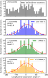 |
Fig. 7 Distribution of longitudinal separation angles between observers’ magnetic footpoints and the associated flare location. Positive (negative) separation angles denote a magnetic footpoint connecting west (east) of the flare longitude. Top: all events, including separation angles of observers not observing an event. Below: longitudinal separation angles of observers who observe a ~100-keV electron event (blue), a ~1-MeV electron event (green), and a > 25-MeV proton event (yellow). |
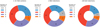 |
Fig. 8 Number of observers per event for > 25 MeV protons (left), ~l-MeV electrons (middle), and ~100 keV electrons (right). |
 |
Fig. 9 Number of events for which an associated flare (left) or an associated type II radio burst (center) was identified. The right-hand plot depicts the fraction of events that were widespread or narrow-spread SEP events. |
6 Summary
We present a new multi-S/C catalog of SEP events detected during solar cycle 25 that reached proton energies of 25 MeV, as was observed by at least two different S/C in the inner heliosphere. The catalog contains key SEP parameters (see Sect. 4) for ∽25–40 MeV protons as well as ~100-keV and ~l-MeV electrons utilizing five different observer locations provided by six space missions; that is, Solar Orbiter, Parker, STEREO A, BepiColombo, SOHO, and Wind, with the latter two both being situated close to the Lagrangian point L1.
Aiming for a most accurate determination of SEP parameters such as onset and peak times, we individually chose the most appropriate time averaging and made use of different viewing directions of the instruments, if those were available, using the viewing direction that was best aligned with the magnetic field during each respective SEP event. For each event, the location of all S/C is provided, regardless of whether one detected the SEP event or not. We also provide the background intensity level in case an observer does not detect the event.
Although each of the SEP events in the catalog is a multi-S/C event, not all of these are observed over a wide longitudinal range. The catalog therefore contains a variety of science cases; for example, widespread SEP events, narrow-spread events, or events with some observers magnetically or radially aligned.
The catalog is provided online as a .csv-file via a citable Zenodo entry (Dresing et al. 2024) and at the SERPENTINE data center. The latter provides in addition a more sophisticated web interface, allowing one to apply various filtering options and to explore the links with other event catalogs provided by the SERPENTINE project, which have a supporting role with respect to the SEP event catalog. These are in situ shock catalogs as well as a catalog of CMEs that were potentially associated with the SEP events. Also available at the SERPENTINE data center are two historic data catalogs based on observations of the Helios S/C: a SEP event catalog and an in situ shock catalog.
Acknowledgements
We acknowledge funding by the European Union’s Horizon 2020 research and innovation program under grant agreement No. 101004159 (SERPENTINE). ND is grateful for support by the Research Council of Finland (SHOCKSEE, grant No. 346902). DEM acknowledges the Academy of Finland project ‘SolShocks’ (grant number 354409). The computer resources of the Finnish IT Center for Science (CSC) and the FGCI project (Finland) are acknowledged. Some of the Parker data analysis is supported by NASA’s Parker Solar Probe Mission, contract NNN06AA01C. Parker Solar Probe was designed, built, and is now operated by the lohns Hopkins Applied Physics Laboratory as part of NASA’s Living with a Star (LWS) program. The ISOIS data are available to the community at https://spacephysics.princeton.edu/missions-instruments/isois; data are also available via the NASA Space Physics Data Facility (https://spdf.gsfc.nasa.gov/). BH, PK and SI thank the German Federal Mnistry for Economic Affairs and Energy and the German Space Agency (Deutsches Zentrum für Luft- und Raum-fahrt, e.V., (DLR)) for their support of Solar Orbiter EPT and HET, STEREO SEPT and SOHO EPHIN under grants number 50OT2002 and 50OC2102. The UAH team acknowledges the financial support by the Spanish Mnis-terio de Ciencia, Innovación y Universidades project PID2019-104863RBI00 /AEI/10.13039/501100011033. The AIP team was supported by the German Space Agency (DLR) under grant numbers 50 OT 1904 and 50 OT 2304. BH acknowledges the support of German research foundation under grant number GI 1352/1-1. We also acknowledge SolarMonitor.org, the online catalog of flares observed by the Hinode satellite, and SpaceWeather prediction Center for providing information about solar flares included in the present catalog. EA acknowledges support from the Academy of Finland/Research Council of Finland (Academy Research Fellow grant number 355659-Project SOFTCAT). The work in the University of Turku and University of Helsinki is performed under the umbrella of Finnish Centre of Excellence in Research of Sustainable Space funded by the Research Council of Finland (2018–2025).
References
- Benkhoff, J., Murakami, G., Baumjohann, W., et al. 2021, Space Sci. Rev., 217, 90 [NASA ADS] [CrossRef] [Google Scholar]
- Dimmock, A. P., Gedalin, M., Lalti, A., et al. 2023, A&A, 679, A106 [NASA ADS] [CrossRef] [EDP Sciences] [Google Scholar]
- Domingo, V., Fleck, B., & Poland, A. I. 1995, Sol. Phys., 162, 1 [Google Scholar]
- Dresing, N., Gómez-Herrero, R., Heber, B., et al. 2014, A&A, 567, A27 [NASA ADS] [CrossRef] [EDP Sciences] [Google Scholar]
- Dresing, N., Kouloumvakos, A., Vainio, R., & Rouillard, A. 2022, ApJ, 925, L21 [NASA ADS] [CrossRef] [Google Scholar]
- Dresing, N., Rodríguez-García, L., Jebaraj, I. C., et al. 2023, A&A, 674, A105 [NASA ADS] [CrossRef] [EDP Sciences] [Google Scholar]
- Dresing, N., Yli-Laurila, A., Valkila, S., et al. 2024, https://doi.org/10.5281/zenodo.10732268 [Google Scholar]
- Fox, N. J., Velli, M. C., Bale, S. D., et al. 2016, Space Sci. Rev., 204, 7 [Google Scholar]
- Gieseler, J., Dresing, N., Palmroos, C., et al. 2023, Front. Astron. Space Sci., 9, 384 [NASA ADS] [CrossRef] [Google Scholar]
- Guo, J., Li, X., Zhang, J., et al. 2023, Geophys. Res. Lett., 50, e2023GL103069 [NASA ADS] [CrossRef] [Google Scholar]
- Hassler, D. M., Zeitlin, C., Wimmer-Schweingruber, R. F., et al. 2012, Space Sci. Rev., 170, 503 [Google Scholar]
- Huovelin, J., Vainio, R., Kilpua, E., et al. 2020, Space Sci. Rev., 216 [CrossRef] [Google Scholar]
- Huttunen-Heikinmaa, K., Valtonen, E., & Laitinen, T. 2005, A&A, 442, 673 [NASA ADS] [CrossRef] [EDP Sciences] [Google Scholar]
- Jakosky, B. M., Grebowsky, J. M., Luhmann, J. G., & Brain, D. A. 2015, Geophys. Res. Lett., 42, 8791 [NASA ADS] [CrossRef] [Google Scholar]
- Jebaraj, I. C., Magdalenic, J., Podladchikova, T., et al. 2020, A&A, 639, A56 [NASA ADS] [CrossRef] [EDP Sciences] [Google Scholar]
- Jebaraj, I. C., Kouloumvakos, A., Magdalenic, J., et al. 2021, A&A, 654, A64 [NASA ADS] [CrossRef] [EDP Sciences] [Google Scholar]
- Jebaraj, I. C., Dresing, N., Krasnoselskikh, V., et al. 2023a, A&A, 680, A7 [Google Scholar]
- Jebaraj, I. C., Kouloumvakos, A., Dresing, N., et al. 2023b, A&A, 675, A27 [NASA ADS] [CrossRef] [EDP Sciences] [Google Scholar]
- Kaiser, M. L., Kucera, T. A., Davila, J. M., et al. 2008, Space Sci. Rev., 136, 5 [Google Scholar]
- Kerdraon, A., & Delouis, J.-M. 1997, in Coronal Physics from Radio and Space Observations, ed. G. Trottet, Lecture Notes in Physics, 483 (Berlin: Springer Verlag) 192 [NASA ADS] [CrossRef] [Google Scholar]
- Kilpua, E. K. J., Good, S. W., Dresing, N., et al. 2021, A&A, 656, A8 [NASA ADS] [CrossRef] [EDP Sciences] [Google Scholar]
- Kilpua, E., Vainio, R., Cohen, C., et al. 2023, Ap&SS, 368, 66 [NASA ADS] [CrossRef] [Google Scholar]
- Kollhoff, A., Kouloumvakos, A., Lario, D., et al. 2021, A&A, 656, A20 [NASA ADS] [CrossRef] [EDP Sciences] [Google Scholar]
- Kollhoff, A., Berger, L., Brüdern, M., et al. 2023, A&A, 675, A155 [NASA ADS] [CrossRef] [EDP Sciences] [Google Scholar]
- Kouloumvakos, A., Rouillard, A., Warmuth, A., et al. 2021, ApJ, 913, 99 [NASA ADS] [CrossRef] [Google Scholar]
- Kouloumvakos, A., Rodríguez-García, L., Gieseler, J., et al. 2022, Front. Astron. Space Sci., 9 [Google Scholar]
- Kouloumvakos, A., Vainio, R., Gieseler, J., & Price, D. J. 2023, A&A, 669, A58 [NASA ADS] [CrossRef] [EDP Sciences] [Google Scholar]
- Krucker, S., Hurford, G. J., Grimm, O., et al. 2020, A&A, 642, A15 [NASA ADS] [CrossRef] [EDP Sciences] [Google Scholar]
- Lario, D., Wijsen, N., Kwon, R. Y., et al. 2022, ApJ, 934, 55 [NASA ADS] [CrossRef] [Google Scholar]
- Lin, R. P., Anderson, K. A., Ashford, S., et al. 1995, Space Sci. Rev., 71, 125 [CrossRef] [Google Scholar]
- Lorfing, C. Y., Reid, H. A. S., Gómez-Herrero, R., et al. 2023, ApJ, 959, 128 [CrossRef] [Google Scholar]
- McComas, D. J., Alexander, N., Angold, N., et al. 2016, Space Sci. Rev., 204, 187 [Google Scholar]
- Morosan, D. E., Carley, E. P., Hayes, L. A., et al. 2019, Nat. Astron., 3, 452 [Google Scholar]
- Morosan, D. E., Pomoell, J., Palmroos, C., et al. 2024, A&A, 683, A31 [NASA ADS] [CrossRef] [EDP Sciences] [Google Scholar]
- Müller-Mellin, R., Kunow, H., Fleissner, V., et al. 1995, Sol. Phys., 162, 483 [CrossRef] [Google Scholar]
- Müller-Mellin, R., Böttcher, S., Falenski, J., et al. 2008, Space Sci. Rev., 136, 363 [Google Scholar]
- Müller, D., St. Cyr, O. C., Zouganelis, I., et al. 2020, A&A, 642, A1 [Google Scholar]
- Nelson, G. J., & Melrose, D. B. 1985, in IN: Solar radiophysics: Studies of Emission from the Sun at Metre Wavelengths (Cambridge and New York: Cambridge University Press), eds. D. J. McLean, & N. R. Labrum, 333 [Google Scholar]
- Ogilvie, K. W., & Desch, M. D. 1997, Adv. Space Res., 20, 559 [Google Scholar]
- Paassilta, M., Papaioannou, A., Dresing, N., et al. 2018, Sol. Phys., 293, 70 [NASA ADS] [CrossRef] [Google Scholar]
- Palmerio, E., Lee, C. O., Mays, M. L., et al. 2022, Space Weather, 20, e2021SW002993 [NASA ADS] [Google Scholar]
- Palmerio, E., Carcaboso, F., Khoo, L. Y., et al. 2024, ApJ, 963 108 [NASA ADS] [CrossRef] [Google Scholar]
- Palmroos, C., Gieseler, J., Dresing, N., et al. 2022, Front. Astron. Space Sci., 9, 395 [NASA ADS] [CrossRef] [Google Scholar]
- Price, D. J., Pomoell, J., & Kilpua, E. K. J. 2022, Front. Astron. Space Sci., 9 [CrossRef] [Google Scholar]
- Raukunen, O., Paassilta, M., Vainio, R., et al. 2020, J. Space Weather Space Clim., 10, 24 [EDP Sciences] [Google Scholar]
- Reames, D. V. 1999, Space Sci. Rev., 90, 413 [NASA ADS] [CrossRef] [Google Scholar]
- Richardson, I. G., & Cane, H. V. 2010, Sol. Phys., 264, 189 [NASA ADS] [CrossRef] [Google Scholar]
- Richardson, I. G., von Rosenvinge, T. T., Cane, H. V., et al. 2014, Sol. Phys., 289, 3059 [NASA ADS] [CrossRef] [Google Scholar]
- Rodríguez-García, L., Balmaceda, L. A., Gómez-Herrero, R., et al. 2023a, A&A, 674, A145 [NASA ADS] [CrossRef] [EDP Sciences] [Google Scholar]
- Rodríguez-García, L., Gómez-Herrero, R., Dresing, N., et al. 2023b, A&A, 670, A51 [NASA ADS] [CrossRef] [EDP Sciences] [Google Scholar]
- Rodríguez-Pacheco, J., Wimmer-Schweingruber, R. F., Mason, G. M., et al. 2020, A&A, 642, A7 [Google Scholar]
- Strauss, R. D., Dresing, N., Kollhoff, A., & Brüdern, M. 2020, ApJ, 897, 24 [NASA ADS] [CrossRef] [Google Scholar]
- Torsti, J., Valtonen, E., Lumme, M., et al. 1995, Sol. Phys., 162, 505 [CrossRef] [Google Scholar]
- Trotta, D., Pecora, F., Settino, A., et al. 2022a, ApJ, 933, 167 [NASA ADS] [CrossRef] [Google Scholar]
- Trotta, D., Vuorinen, L., Hietala, H., et al. 2022b, Front. Astron. Space Sci., 9, 1005672 [NASA ADS] [CrossRef] [Google Scholar]
- Trotta, D., Horbury, T. S., Lario, D., et al. 2023a, ApJ, 957, L13 [CrossRef] [Google Scholar]
- Trotta, D., Pezzi, O., Burgess, D., et al. 2023b, MNRAS, 525, 1856 [NASA ADS] [CrossRef] [Google Scholar]
- Trotta, D., Hietala, H., Horbury, T., et al. 2023c, MNRAS, 520, 437 [NASA ADS] [CrossRef] [Google Scholar]
- Trotta, D., Larosa, A., Nicolaou, G., et al. 2024, ApJ, 962, 147 [CrossRef] [Google Scholar]
- von Rosenvinge, T. T., Reames, D. V., Baker, R., et al. 2008, Space Sci. Rev., 136, 391 [Google Scholar]
- van Haarlem, M. P., Wise, M. W., Gunst, A. W., et al. 2013, A&A, 556, A2 [NASA ADS] [CrossRef] [EDP Sciences] [Google Scholar]
- Watanabe, K., Masuda, S., & Segawa, T. 2012, Sol. Phys., 279, 317 [NASA ADS] [CrossRef] [Google Scholar]
- Wijsen, N., Lario, D., Sánchez-Cano, B., et al. 2023, ApJ, 950, 172 [NASA ADS] [CrossRef] [Google Scholar]
- Wraase, S., Heber, B., Böttcher, S., et al. 2018, A&A, 611, A100 [NASA ADS] [CrossRef] [EDP Sciences] [Google Scholar]
- Xiao, H., Maloney, S., Krucker, S., et al. 2023, A&A, 673, A142 [NASA ADS] [CrossRef] [EDP Sciences] [Google Scholar]
Assuming a spectral index of −3 results in a mean energy of 1.02 MeV, while a spectral index of −1.5 yields a mean energy of 1.95 MeV.
All times in the catalog (except the inferred SEP injection times) refer to their measurement at the S/C.
All coordinates of the catalog are provided in the Carrington coordinate system
In cases of backside flares, which were not observed by GOES we use Solar Orbiter/STIX observations, if available. An estimated GOES class is then provided based on the counts in the STIX 4-10 keV channel (see Sect. 4.1).
We use S/C names or ‘GB’ for ground-based observations of metric type II bursts.
Radio comments provide the instrument used for metric type II burst identification or S/C data availability notes.
These CMEs are listed in the SERPENTINE CME catalog at https://data.serpentine-h2020.eu/catalogs/cme/
These shocks are searched in association with the events and are listed in the SERPENTINE IP shock catalog at https://data.serpentine-h2020.eu/catalogs/shock-sc25/.
The uncertainty of the injection time is at least as high as the time averaging used to determine the corresponding onset time.
Based on measurements at the S/C. If empty, a nominal value of 400 km s−1 was used.
In case of Parker the comments also contain a remark if the S/C was not nominally orientated.
ftp://ftp.swpc.noaa.gov/pub/indices/events/
https://github.com/hayesla/stix_flarelist_science. The STIX flare list was created by the STIX ground software and data processing team (Xiao et al. 2023).
We used the plots provided at https://parker.gsfc.nasa.gov/crocs.html
In case of Parker observations we do not provide the background intensity for electrons as those data were not made public yet at the time of writing.
All Tables
Energetic particle instruments, their available viewing directions, and energy channels used for the catalog.
Energetic particle instruments, energy channels, and corresponding mean energies used to determine the electron-to-proton ratios.
All Figures
|
Fig. 1 Multi-S/C events of February 24 and 25, 2023. The top plot presents the longitudinal configuration of S/C in the heliographic equatorial plane with respect to the longitude of the associated flare (black arrow) for the event starting on 24 February. The plot was produced with the Solar-MACH tool (Gieseler et al. 2023). The colored spirals denote the magnetic field lines connecting each observer with the Sun. The dashed black spiral represents the field line connecting with the flare. The bottom plot shows the intensity time series of ~100-keV electrons (top), ~1-MeV electrons (middle), and >25-MeV protons (bottom). Parker did not observe the events but a previous event happening earlier on 24 February. Since there is no obvious electron foreground in the EPI-Lo electron measurements (top panel) during the second event, the counts during this time period are background, assumed to be primarily caused by galactic cosmic rays. Parker/HET data were not available during the shown time period. The black arrow on top of the upper panel denotes the times of the associated flares. Solid (dotted) lines mark the onset (peak) times, with colors corresponding to those of the S/C time series. |
| In the text | |
|
Fig. 2 Figure structure as in Fig. 1, but for the event of March 28, 2022. This event was only observed by STEREO A and near-Earth S/C (Wind and SOHO), but not at Solar Orbiter or Parker (BepiColombo/SIXS data were not available). The science case of this event is a “narrow-spread event.” |
| In the text | |
|
Fig. 3 Starting page of the multi-S/C SEP event catalog at the SERPENTINE data center. Various filtering options can be applied by the user. Below, the resulting list of events, including several of the main event parameters, is shown. |
| In the text | |
|
Fig. 4 Detailed view of a selected event at the SERPENTINE data center. This page shows all parameters of the selected event. |
| In the text | |
|
Fig. 5 Top: highest > 25 MeV-proton peak intensity observed (black dots) in each event as a function of time, with widespread events marked in red. Daily and monthly sunspot numbers are shown by gray curves (right axis) provided by WDC-SILSO, Royal Observatory of Belgium, Brussels. Bottom: histogram of event occurrences, with all events in gray, widespread events in red, and narrow-spread events in blue. |
| In the text | |
|
Fig. 6 Histogram of S/C distances during event observations for the three different energy-species combinations. |
| In the text | |
|
Fig. 7 Distribution of longitudinal separation angles between observers’ magnetic footpoints and the associated flare location. Positive (negative) separation angles denote a magnetic footpoint connecting west (east) of the flare longitude. Top: all events, including separation angles of observers not observing an event. Below: longitudinal separation angles of observers who observe a ~100-keV electron event (blue), a ~1-MeV electron event (green), and a > 25-MeV proton event (yellow). |
| In the text | |
|
Fig. 8 Number of observers per event for > 25 MeV protons (left), ~l-MeV electrons (middle), and ~100 keV electrons (right). |
| In the text | |
|
Fig. 9 Number of events for which an associated flare (left) or an associated type II radio burst (center) was identified. The right-hand plot depicts the fraction of events that were widespread or narrow-spread SEP events. |
| In the text | |
Current usage metrics show cumulative count of Article Views (full-text article views including HTML views, PDF and ePub downloads, according to the available data) and Abstracts Views on Vision4Press platform.
Data correspond to usage on the plateform after 2015. The current usage metrics is available 48-96 hours after online publication and is updated daily on week days.
Initial download of the metrics may take a while.