| Issue |
A&A
Volume 687, July 2024
|
|
|---|---|---|
| Article Number | A169 | |
| Number of page(s) | 17 | |
| Section | Astrophysical processes | |
| DOI | https://doi.org/10.1051/0004-6361/202348069 | |
| Published online | 05 July 2024 | |
Multi-wavelength pulse profiles from the force-free neutron star magnetosphere
Université de Strasbourg, CNRS, Observatoire astronomique de Strasbourg, UMR 7550, 67000 Strasbourg, France
e-mail: This email address is being protected from spambots. You need JavaScript enabled to view it.
Received:
26
September
2023
Accepted:
8
April
2024
Abstract
Context. The last two decades have witnessed dramatic progress in our understanding of neutron star magnetospheres thanks to force-free and particle-in-cell simulations. However, the associated particle dynamics and its emission mechanisms and locations have not been fully constrained, notably in X-rays.
Aims. In this paper, we compute a full atlas of radio, X-ray, and γ-ray pulse profiles, relying on the force-free magnetosphere model. Our goal is to use such a data bank of multi-wavelength profiles to fit a substantial number of radio-loud γ-ray pulsars that have also been detected in non-thermal X-rays to decipher the X-ray radiation mechanism and sites. Using results from the third γ-ray pulsar catalogue (3PC), we investigate the statistical properties of this population.
Methods. We assume that radio emission emanates from field lines rooted to the polar caps, at varying height above the surface, close to the surface, at an altitude about 5–10% of the light cylinder radius, r L. The X-ray photons are produced in the separatrix region within the magnetosphere; that is, the current sheet formed by the jump from closed to open magnetic field lines. We allow for substantial variations in emission height. The γ-rays are produced within the current sheet of the striped wind, outside the light cylinder.
Results. A comprehensive set of radio, X-ray, and γ-ray light curves was computed. Based on only geometric considerations about magnetic obliquity, line-of-sight inclination, and the radio beam cone opening angle, pulsars can be classified as radio-loud or quiet and as γ-ray-loud or quiet. We found that the 3PC sample is compatible with an isotropic distribution of obliquity and line of sight.
Conclusions. The atlases constructed in this work are the fundamental tools with which to explore individual pulsars and fit their multi-wavelength pulse profiles in order to constrain their magnetic topology, the emission sites, and the observer’s line of sight.
Key words: acceleration of particles / magnetic fields / radiation mechanisms: non-thermal / methods: numerical / pulsars: general
© The Authors 2024
 Open Access article, published by EDP Sciences, under the terms of the Creative Commons Attribution License (https://creativecommons.org/licenses/by/4.0), which permits unrestricted use, distribution, and reproduction in any medium, provided the original work is properly cited.
This article is published in open access under the Subscribe to Open model. This email address is being protected from spambots. You need JavaScript enabled to view it. to support open access publication.
1. Introduction
Today, almost 300 γ-ray pulsars have been reported in the Fermi pulsar catalogue1; it is also worth viewing the third pulsar catalogue detailed in Smith et al. (2023). Among them, more than 20 were detected pulsating simultaneously in radio and X-ray. This population of pulsars is a perfect target to study the multi-wavelength emission properties of neutrons stars. The complete list of radio pulsars has been compiled in the ATNF Pulsar Catalogue of Manchester et al. (2005) and is kept up to date online. Unfortunately, no exhaustive non-thermal X-ray pulsar catalogue exists to date. However, some recent papers like Coti Zelati et al. (2020) acknowledge the simultaneous detection of non-thermal X-rays and γ-rays of a significant sample of 40 pulsars. Chang et al. (2023) found 32 pulsars described by a power law (PL) + black body (BB) model. A single PL model fits the other 36 pulsars well (thus 68 in total). These numbers are however only lower limits because very recently Mayer & Becker (2024) identified several dozen possible X-ray pulsars of the unassociated Fermi-LAT sources with SRG/eROSITA (Spektrum-Roentgen-Gamma, extended ROentgen Survey with an Imaging Telescope Array), about 30–40 candidates distributed equally in young and recycled pulsars. In the higher energy band of soft γ-rays, another useful list of pulsars is given by Kuiper & Hermsen (2015). Phase-aligned multi-wavelength pulsar light curves are the milestones to constrain the location of radio, X-ray, and γ-ray emission within the magnetosphere and near wind, and attempts have been made to compute them for several decades.
One of the most promising joint radio and γ-ray model relies on pulsar striped wind geometry. This idea has been investigated in depth over the last two decades, starting with Kirk et al. (2002). It was then applied to the Fermi γ-ray pulsars by Pétri (2011) in the split monopole picture, or more recently by Benli et al. (2021) and Pétri & Mitra (2021) in the force-free dipole magnetosphere. These works showed that a joint radio+γ-ray pulse profile fitting can drastically constrain the magnetic dipole moment inclination angle with respect to the rotation axis as well as the line-of-sight inclination angle. These fittings were based on numerical quantitative simulations of the force-free magnetosphere performed by Pétri (2012). These kinds of numerical simulations were pioneered by Contopoulos et al. (1999) for the axisymmetric magnetosphere and extended by Spitkovsky (2006) to an oblique rotator. However, strictly speaking, the force-free model does not radiate because it is dissipationless as no particle acceleration occurs. Therefore, the paradigm shifted to a kinetic description of these magnetospheres including single particle acceleration in 3D (Philippov et al. 2015) and self-consistent radiation feedback to predict observational signatures (Cerutti et al. 2016b) that even predict the polarisation properties (Cerutti et al. 2016a). The striped wind and its dissipation was also investigated by particle in cell (PIC) simulations in Cerutti & Philippov (2017), Cerutti et al. (2020). Sticking closer to γ-ray observations, Brambilla et al. (2018), Kalapotharakos et al. (2017), and Kalapotharakos et al. (2018) performed similar simulations.
Several other emission regions were proposed in the past. The outer gaps, the slot gaps, and the polar caps are the favourite places for pulsed emission. They predict distinct pulse profiles, helping one to discriminate between competing models (Dyks & Rudak 2003; Dyks et al. 2004). Producing exhaustive atlases of light curves in all relevant wavelengths is the starting point for any broadband fitting task. For instance, Watters et al. (2009) focused on young γ-ray pulsar profiles and Pierbattista et al. (2015, 2016) on different emission mechanisms for a significant sample of pulsars, whereas Johnson et al. (2014) focused on millisecond pulsars. Two-pole caustics and outer gap atlases were presented in Harding et al. (2011).
The third Fermi γ-ray pulsar catalogue (Smith et al. 2023) summarises all our knowledge about γ-ray pulsar spectra and light curves. Because force-free computations do not catch the acceleration and radiation mechanism within the magnetosphere and wind, resistive or dissipative magnetospheres were built, like the Force-free Inside, Dissipative Outside (FIDO) model introduced by Kalapotharakos et al. (2012), and used by Brambilla et al. (2015) for detailed pulsed γ-ray investigations (for some reviews on the interplay between magnetospheric modelling and γ-ray observations, see Harding (2016) and Venter et al. (2018)).
Whereas more than 3000 pulsars are known to be radio emitters, only 10% of them are seen shining in γ-rays. The release of the third pulsar catalogue by Smith et al. (2023) furnishes a wealth of new and accurate data, helping in our task to decipher the high-energy radiation mechanism and location. Although many studies focused on the radio and γ-ray emission, using fluid or particle simulations (Cerutti et al. 2016b; Kalapotharakos et al. 2017, 2023; Watters et al. 2009; Pierbattista et al. 2016), none really addressed the pulsed X-ray emission properties. This article fills the gap by exploring quantitatively the X-ray light curves’ morphology depending on the pulsar geometry.
Section 2 reminds us of the emission locations of the different energy bands: radio, X-rays, and γ-rays. Next, Sect. 3 summarises the light curves in these respective wavebands. Section 4 discusses the energetics of the radiating particles by computing the curvature of field lines and the associated photon energy and particle dynamics. Some statistical expectations are compared to the current observational status in Sect. 5. Conclusions and future perspectives are presented in Sect. 6.
2. Emission sites
In recent years, three standard emission sites have emerged from different studies of the pulsar magnetosphere. The first one is the polar cap region, which is close to the stellar surface and responsible for the coherent radio emission. The second one follows the region along the separatrix; that is, the transition surface between close and open magnetic field lines within the light cylinder. The third one radiates in the current sheet of the pulsar striped wind. We briefly go over here the main features of such emission regions, which have been introduced in a similar way by Pétri (2018), including general relativistic effects.
The set-up assumes that the magnetic dipole moment, μ, is directed along a unit vector, m, such that μ = μ m. This magnetic moment rotates at an angular speed, Ω, around the rotation axis directed along the vector, ez, of the Cartesian basis vectors (ex, ey, ez). The observer line-of-sight unit vector points towards the direction, n. The emitting particle density number, n, is assumed to be spherically symmetric and to decrease like a power law in spherical radius, r, with an exponent, q, such that
 (1)
(1)
The particle density number is therefore prescribed; we set q = 2 in all wavelengths. The Lorentz factor of the moving particles was set to Γ = 10.
2.1. Magnetic field geometry
The structure of the magnetic field lines fully determines the size and location of the polar cap, the geometry of the separatrix surface, and the location of the current sheet within the striped wind. These are the three sites producing, respectively, radio photons, X-rays, and γ-rays. Our model is based on numerical simulations of the neutron star magnetosphere using spectral methods in the force-free approximation, updating previous computations performed by Pétri (2012) and Pétri & Mitra (2021). The ratio between the neutron star radius, R, and the light cylinder radius, rL, was set to R/rL = 0.1, corresponding to the altitude where radio emission was expected to be produced. Close to the surface, the magnetic field is reminiscent to a static dipole corotating with the star, whereas outside the light cylinder magnetic field lines open up and form a current sheet wobbling around the equatorial plane. An example of field lines in the equatorial plane for an χ = 90° obliquity is shown in Fig. 1.
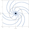 |
Fig. 1. Magnetic field lines in the equatorial plane for an orthogonal rotator with R/rL = 0.1. The neutron star is shown as a black disk and the light cylinder as a dashed black circle. |
2.2. Polar cap and radio
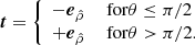
A careful analysis of emission height in normal pulsars based on the rotating vector model and using a large sample of radio pulsars (Weltevrede & Johnston 2008; Mitra 2017; Johnston & Karastergiou 2019; Johnston et al. 2023) showed that radio emission is emanating from regions well above the polar caps, around 5%–10% of the light cylinder radius. For pulsars showing interpulses, the geometry is even better constrained, because they are close to orthogonal rotators (Johnston & Kramer 2019). We used this proxy to implement a simple radio pulse profile emissivity that drops as a Gaussian when moving away from the magnetic axis. The width of the pulse profile is defined by the typical half-opening angle of the emission cone at an altitude, he, above the stellar surface,
 (2)
(2)
with the half-opening angle of the cone locating the root of the field lines as
 (3)
(3)
The emissivity within the radio-emitting region and related to the Gaussian beam shape reads
 (4)
(4)
Radio photons are assumed to be produced at a small emission height interval starting from the inner boundary of the simulation box, he = R1. In the present simulations, this was set to R1/rL = 0.1, and thus 10% of the light cylinder radius, as was found in the above-mentioned literature. The extension in the radius was set to 1% of rL, amounting to a height range of [0.1, 0.11] rL. As the magnetic moment, m, rotates, the dot product, m ⋅ n, evolves with time according to Ω t and reaches its maximal value whenever ez, m, and n are coplanar. This occurs whenever the north or south pole points towards the observer. Photons are emitted along the local particle velocity vector, v, which is a combination of corotation velocity and velocity along magnetic field lines such that
 (5)
(5)
The unknown parameter, f, is found by imposing the Lorentz factor, Γ, of the particle, all other quantities being known. Expression (5) takes into account the aberration effect through the corotating velocity field in the first term of the right-hand side. Retardation is included through the time of flight delay of photons. These aberration or retardation effects are discussed in Blaskiewicz et al. (1991).
2.3. Separatrix and X-rays
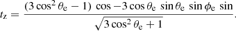
Farther away from the radio-emitting region, in the separatrix zone where the transition between close and open magnetic field lines occurs, we expect X-rays photons to be produced from the synchrotron and/or curvature radiation mechanism. This X-ray component is produced by the secondary electron-positron pairs radiating synchrotron photons. For instance, Kisaka & Tanaka (2014) computed the synchrotron emission for old pulsars to explain the non-thermal X-ray emission, whereas Kisaka & Tanaka (2017) investigated a similar mechanism to estimate the efficiency of this emission in rotationally powered pulsars. Takata & Cheng (2017) discussed the connection between X-ray and GeV emission in this framework. Torres et al. (2019) show that the synchro-curvature radiation is able to explain the non-thermal X-ray spectra of several pulsars but they did not compute pulse profiles (see also some refinement by Íñiguez Pascual et al. 2022). For polar cap and outer gap scenarios of non-thermal X-ray pulsed emission, see also Peng & Zhang (2008) and Zhang & Jiang (2006). In a narrow layer of small thickness parametrized by σsep (much less than the light cylinder radius) and delimited by magnetic flux tubes, with a constant emissivity along field line but decaying like a Gaussian for field lines moving away from the separatrix surface, X-ray photons start propagating tangentially to the local direction of the velocity vector (Eq. (5)) where they were generated. More precisely, the emissivity of a given point attached to a field line reads
 (6)
(6)
where ℓmin is the minimal distance of this field from the light cylinder. By construction, any point on this field line will have the same emissivity as another point on the same field line except for a modulation by the particle density number, n(r). The locations of the X-ray emission sites are largely unconstrained so far. In order to get an idea of the emission height and extension, we divided the separatrix from the inner boundary simulation box to the light cylinder into a set of uniform intervals of radial length 0.1rL, from r = R1 to r = rL. As the radiation is additive, any realistic light curve is given by summing several adjacent regions to construct the total light curve from the individual building block light curves. In this manner, we deduced the lower and the upper emission heights along the separatrix surface.
2.4. Striped wind and γ-rays
The most energetic photons are produced in the current sheet of the striped wind, outside the light cylinder. Emission starts straight from the light cylinder up to several rL, with an emissivity decaying with distance due to the decreasing particle density number, n(r). The emitting current sheet is supposed to be infinitely thin and located in space, where the radial component of the magnetic field changes sign between the upper part,  (connected to the north pole), and the lower part,
  (connected to the south pole), such that
  . The locus thus formed corresponds to a surface like a ballerina skirt, similar to the solar wind structure. The emissivity therefore vanishes out of the surface defined by the current sheet and equals
 (7)
(7)
on this surface. The emission starts outside the light cylinder at cylindrical distances, r sin θ ≥ rL, and the wind propagates radially at a Lorentz factor, Γ, fixed to Γ = 10. No other free parameter is required in this minimal model. The base of the radiating wind, rin, is located outside the light cylinder and extends to a spherical radius, rout > rin. This outer boundary is not constrained but the wind emissivity decreases with the distance, r, and the current sheet geometry slightly changes, based on the magnetic topology. At large distances, its luminosity becomes negligible, so we arbitrarily cut the wind at a variable radius, rout, in order to quantify the impact of the emission height in γ-rays onto the light curves. Therefore, we defined two intervals, a first at [1, 2]rL and a second at [2, 3]rL, comparing the evolution of the light curves with distances.
3. Multi-wavelength radiation patterns
In this section, we discuss in depth the multi-wavelength pulse profile characteristics and evolution with the geometry controlled by the obliquity, χ, and the line-of-sight inclination angle, ζ. First, we summarise all of the results by plotting intensity maps in radio, X-ray, and γ-ray. Next, we show typical atlases of light curves by varying χ and ζ. Finally, for a given geometry with fixed values of χ and ζ, we investigate the pulse shape dependence on the emission height, especially in X-rays, where these variations with altitude are most prominent.
3.1. Geometric constraints
Due to the particular configuration of the polar cap and the striped wind emission, it is possible to derive simple relations between the obliquity and the line-of-sight inclination to decide if radio and/or γ-ray photons are detected or not. For X-ray detection, the criteria is more difficult to derive.
The current sheet of the striped wind crosses the observer’s line of sight whenever the latter lies close to the equatorial plane; that is,
 (8)
(8)
This condition is derived in Pétri (2011) for the split monopole solution that does not significantly differ from the dipole force-free model obtained by the numerical solution. This condition is very general as it does not depend on the exact nature of the field line geometry inside the light cylinder as long as the dominant multipole becomes the dipole at the light cylinder. For a radio emission cone of the half-opening angle, ρ, the visibility condition for one pole reads
 (9)
(9)
whereas for the other pole it becomes
 (10)
(10)
This is due to the symmetry between the angle, χ, and π − χ when considering the emission patterns of the magnetosphere. To observe two radio pulses, both conditions must be satisfied simultaneously, leading to the constraint
 (11)
(11)
In other words, the line of sight must not deviate from the equatorial plane more than the radio emission cone half-opening angle. A second condition on the obliquity must be met:
 (12)
(12)
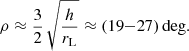
meaning that it must be almost an orthogonal rotator, within an interval equal to twice the radio cone half-opening angle. The value of ρ is directly related to the emission height, he, given by Eq. (2). Radio observations suggest that he/rL ≲ 0.1; thus, ρ ≲ 27.6°.
Figure 2 summarises the constraints about radio and γ-ray visibility depending on χ and ζ. The red area corresponds to only γ-ray, the blue area to only radio, and the magenta area to radio-loud γ-ray visibility. The observer looks exactly onto the magnetic axis when the geometry falls onto one of the two dashed diagonals, ζ = χ or ζ = π − χ. The pattern is highly symmetric due to the north-south symmetry of the magnetic field and due to the stellar rotation. For instance, χ = π/2 and ζ = π/2 are symmetry axes.
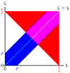 |
Fig. 2. Geometry showing the region of radio and γ-ray visibility depending on the magnetic obliquity, χ, and line of sight, ζ. The red area corresponds to γ-ray-only, the blue area to radio-only with ρ = 20°, and the magenta area to radio-loud γ-ray visibility. Due to the symmetry of the plot, the three other quadrants with χ ≥ π/2 or ζ ≥ π/2 are not shown. |
For the X-ray constraints, finding a simple analytical condition for visibility is impossible because the exact geometry of the separatrix is not known in the force-free model. However, to make progress in this direction and derive an approximate expression for detecting pulsed X-rays, we assume that the photons emanate from well within the light cylinder at distances of r ≲ rL. In this region, the magnetic field remains dipolar to an acceptable precision and the polar cap size and shape still resemble the vacuum case, although deviations are observed, as has been checked in several previous works (for recent results, see for instance Fig. 11 of Pétri 2022a where quantitative comparisons have been done). We therefore used the static dipolar separatrix structure as a proxy to predict the pulsed X-ray detectability. To study the impact of the dipolar geometry, we used dipolar coordinates, which are detailed in the Appendix B and which were used by Swisdak (2006), Orens et al. (1979). In this dipole approximation, the condition for pulsed X-ray detection mimics the radio visibility condition, the only difference being the size of the emitting cone because of the varying emission altitude postulated in X-rays and the fact that the cone is hollow. However, because of the stellar rotation, even a hollow cone will cross the line of sight when the condition
 (13)
(13)
is fulfilled, ρX being the maximum X-ray emission cone half-opening angle. It depends on the boundaries of the emitting region located between the radii h1 and h2. Actually, because ρX is a monotonic function of he, it increases with he and the maximum is given by
 (14)
(14)
the cone opening angle at lower altitude always being smaller.
3.2. Maps
Figure 3 shows the multi-wavelength maps of radio, X-ray, and γ-ray emission. In the left column, the radio emission is produced in the range r/rL ∈ [0.1, 0.11], and in the second column, the non-thermal X-ray is produced from an emission height in r/rL ∈ [0.2, 0.3], whereas the third column assumes the same emission in r/rL ∈ [0.5, 0.6]. In the last two columns the γ-ray emission emanates from the intervals r/rL ∈ [1, 2] and r/rL ∈ [2, 3], respectively. We observe the archetypal S-shape pattern produced by the striped wind structure. The high-energy emission pattern is not significantly sensitive to the emission height, as long as the radiation sites remain close to the light cylinder. The contributions for large distances are smeared out and decay quickly with radius due to the density dependence, n(r). For r/rL ≳ 3 − 4, the emission produced becomes insignificant, without having any impact on the light curves, and thus it was discarded.
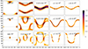 |
Fig. 3. Map of radio, X-ray, and γ-ray radiation for different emission altitudes and for χ = {15°,45°,75°}. The legend shows the wavelength, emission interval, and obliquity. Maximum intensities are normalized and colour-coded in the right legend. |
At low altitudes of r/rL ∈ [0.1, 0.2], the X-ray emission pattern looks like an oval encircling the radio emission pattern. As the height increases, this pattern approaches the S-shape pattern of the striped wind. The dependence on altitude is important in X-ray because it follows the drastically changing magnetic field topology within the light cylinder, from an almost static dipole configuration close to the surface to a retarded dipole close to the light cylinder, transitioning to an electromagnetic wave outside it.
The above maps give a full representation of the whole set of light curves being produced in the different emission sites. In the next paragraph, we show atlases of radio, X-ray, and γ-ray light curves to be used in fitting multi-wavelength pulse profiles of radio-loud γ-ray pulsars also detected in non-thermal X-rays. A detailed example will be discussed in another paper.
3.3. Light curves
All of the possible radio pulse profiles from a centred dipole are shown in Fig. A.1. For an almost aligned rotator, the pulsed fraction is weak at all line-of-sight inclination angles, ζ, and the pulsation is hardly detectable, depending on the noise level. When far from an orthogonal rotator, only one pulse is visible from one magnetic pole. Only for ζ ≈ 90° are both pulses visible and separated by half a period, due to the symmetry of the dipole field. The detection of a double pulse structure depends on the angles (χ,ζ) but also on the beam width. In the special case of ζ = 90°, both pulses are symmetrical and always detected whatever ζ. For lower obliquities of ζ ≲ 90°, one pulse dominates; see for instance the case {χ,ζ} = {75°,80°,}.
The γ-ray light curves are shown in Fig. A.2. Inspecting this figure with r/rL ∈ [1, 2], the pattern shows one peak or two peaks depending on the peculiar combination of {χ,ζ}. It behaves similarly to the radio pulse profile. However, in the γ-ray band, there is much more chance of producing a double-peaked light curve because this configuration is much more favourable geometrically. A double peak is observed whenever |ζ − π/2| ≤ χ. Moving to higher altitudes in the range r/rL ∈ [2, 3] does not alter these findings (Fig. A.2).
The new part of this work concerns the X-ray radiation, which is supposed to be produced along the separatrix, on an unspecified altitude that is left as a free parameter. At the lowest altitude, in the range r/rL ∈ [0.1, 0.2], the pulse profiles look like they do in Fig. A.3. We observe between one and four pulses, depending on the geometry. A single pulse is observed for low obliquity and low line-of-sight inclination, in the upper left corner of the plot, whereas four pulses are observed at high obliquity (close to an orthogonal rotator) and high line-of-sight inclination angles. At higher altitudes, for instance in the range r/rL ∈ [0.4, 0.5], the four peaks transform into a double peak profile (Fig. A.4).
We plan to use these X-ray atlases to constrain the emission location of the X-ray photons. To this end, we assume that the pulsar obliquity is well determined by the joint radio and γ-ray pulse profile fitting, extracting accurate values for both angles, χ and ζ. Then, to estimate the X-ray emission height, it is sufficient to explore a small subset of the entire X-ray atlas. As an example, we show the evolution of the pulse profile with minimum and maximum altitudes h1 and h2 in Fig. A.5 for a pulsar with obliquity χ = 45°.
4. Radiation energetics
The geometric approach of fitting light curves is not sufficient to grasp all the dynamics of particle acceleration and radiation within the magnetosphere and wind. The energetic considerations of the whole electrodynamic process is another important aspect of the problem that we discuss in this section.
4.1. Curvature of field lines
Well inside the light cylinder, where the radio emission is produced, to a good accuracy, the magnetic field follows the static dipole geometry. To estimate quickly the curvature of field lines near the surface, along the separatrix and inside the radio emission beam, we started by computing the static dipole curvature. For an aligned dipole, each field line is labelled by a parameter, λ, such that
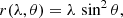 (15)
(15)
r being the radius and θ the azimuth in a spherical coordinate system. Along this particular field line symbolised by λ, the curvature radius, ρc, depends on θ as
 (16)
(16)
Along the magnetic axis, the curvature vanishes, but as we will show, for the rotating dipole, the curvature does not vanish due to magnetic sweep-back. By construction, the separatrix is defined by field lines satisfying λ = rL. Close to the polar caps, the angle, θ, is small and the curvature tends to
 (17)
(17)
which at the stellar surface gives  , and therefore
 (18)
(18)
The neutron star radius, R, being fixed to an almost constant value of R ≈ 12 km, the curvature radius increases according to  . The curvature radius increases with the pulsar period; thus, the frequency of curvature radiation diminishes right at the surface. In order to keep a typical radio photon range in the interval [10 MHz, 10 GHz], the emission altitude must increase too.
The curvature, κc = 1/ρc, along the separatrix is shown in Fig. 4, in units of 1/rL for the vacuum Deutsch solution (VAC) in blue and for the force-free magnetosphere (FFE) in orange. The inner boundary of the simulation box has been fixed to R1/rL = 0.1. The curvature decreases with distance to the star like r−1/2 for the vacuum and approximately the same law, ∼r−1/2, for the FFE, as long as r ≪ rL. This behaviour was expected, as well inside the light cylinder the influence of rotation and magnetospheric currents becomes negligible, the first being of order (R/rL)2 and the second of order (R/rL). The FFE case produces higher curvature because of the stronger magnetic field sweep-back due to the current flowing along field lines. For R1/rL = 0.1, typical values at this emission height are κc rL ≈ 2.4.
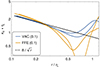 |
Fig. 4. Curvature in units of 1/rL along the separatrix, starting from the surface going to the light cylinder and back to the surface for the vacuum field (VAC, in orange) and the force-free solution (FFE, in blue). Values are shown for an obliquity of χ = 75°. |
The behaviour of the curvature, κc, along the central magnetic field line is very different, as is shown in Fig. 5, in units of 1/rL, for the VAC in blue and for the FFE in orange. The curvature increases with distance to the star like r2 for the vacuum and like r1/2 for the FFE, as long as r ≪ rL. This is in contradiction with the radius-to-frequency mapping because the high-frequency photons are produced at a higher altitude in this picture. We therefore anticipate an opposite variation of the radio pulse width between the core and the cone components, as has been observed in some pulsars taken from the literature. Indeed, Posselt et al. (2021) found a sample of pulsars showing the opposite of the radius to frequency mapping (RFM) prediction, which is a pulse width increase with frequency. Similar conclusions have been drawn by Johnston et al. (2008), who claimed that almost one third of their sample disagrees with RFM. Chen & Wang (2014) reported the same trend for about 20% of 150 pulsars analysed (see also Noutsos et al. 2015). For a given frequency, the cone and core components emanate from different altitudes. A last important point concerns the possible phase lag between radio pulses in different frequency bands. Indeed, if emitted at different altitudes along the magnetic axis, because of the increase in bent field lines, we should relate this lag to the difference in altitude, as was already mentioned by Phillips (1992). To this end, we plot the angle between the local magnetic field at a radius, r, and the magnetic moment direction for VAC and FFE, as is shown in Fig. 6. The difference between VAC and FFE is significant, a factor of ten or more. Differences in emission altitudes will not only impact the width of the pulse profiles because of the increase in the radio cone beam opening angle, but also the phase of their centre due to the magnetic field sweep-back.
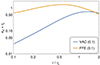 |
Fig. 5. Curvature of the magnetic axis for the VAC and the FFE. Values are shown for an obliquity of χ = 75°. |
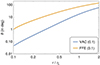 |
Fig. 6. Angle between the local magnetic field at radius r for points on the central field line and the magnetic moment direction for the VAC and the FFE. Values are shown for an obliquity of χ = 75°. |
4.2. Broadband photon emission
From a theoretical point of view, in the pair cascade region above the polar cap, current models predict two populations of pair plasma flows: a primary beam of electrons and positrons with a very high Lorentz factor and accelerated in the vacuum gap potential drop to reach γb ≈ 106, and a secondary plasma of e± pairs produced by cascades due to magnetic photo-disintegration reaching Lorentz factors of γp ≈ 102 (Kazbegi et al. 1991; Arendt & Eilek 2002; Usov 2002). In the partially screened gap model of Gil et al. (2003), an ion outflow is allowed, with γion ≈ 103. Electrons and positrons do not follow exactly the same distribution functions because of the parallel electric field screening (Beskin et al. 1993). The pair multiplicity factor can reach values up to κ ≈ 104 − 105 (Timokhin & Harding 2019). This pair plasma produces the observed radio emission, typically in the MHz–GHz band, through curvature radiation (Mitra 2017).
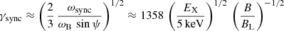
On top of the primary and secondary beams, three different sites produce photons at different energies. Radio emission is a consequence of curvature radiation along open magnetic field lines close to the polar caps. The Lorentz factors require it to emit typically at a frequency of 1 GHz at a height of r/rL ≈ 0.1, where the curvature is about κc rL = rL/ρc ≈ 30, are
 (19)
(19)
which corresponds to the secondary plasma flow, as was expected.
For the X-ray photons, we could either invoke synchrotron radiation or curvature radiation. The particle Lorentz factor to produce typically a 5 keV photon must be in either case
 (20a)
(20a)
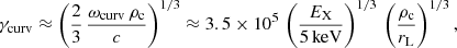 (20b)
(20b)
where ψ is the particle pitch angle with respect to the magnetic field line and EX the photon energy. For the numerical value, we used the most favourable pitch angle of ψ = 90°. However, synchrotron radiation is very unlikely because particles stay in their fundamental Landau level up to the light cylinder.
If the X-ray photons are produced in regions with a similar curvature to radio photons, then the particle Lorentz factor ratio must be
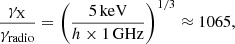 (21)
(21)
which corresponds to the primary beam, with a low Lorentz factor of about 104 − 5. Therefore, radio and non-thermal X-ray emission are produced by curvature radiation of the secondary plasma (γb ≈ 100) and the primary beam (γp ≳ 105), respectively. This is consistent with the 1D particle distribution function of the out-flowing relativistic plasma along open magnetic field lines. Moreover, above a height of 0.5 rL, the sharp decrease in the curvature, κc, shifts the photon energy to a lower band well below 1 keV. In addition, the particle density number drops due to the divergent magnetic field geometry and the spherical expansion.
The reason why non-thermal X-rays are mostly produced along the separatrix is twofold. First, the curvature radiation power scales as the curvature squared,  , and the particle charge squared, q2, such that
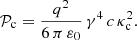 (22)
(22)
Because the curvature, κc, drastically decreases towards the centre of the polar cap, the associated curvature power also decreases, even faster than κc. This leads to a hollow cone model reminiscent of the radio hollow cone model. Second, the particle density number, ne, along the separatrix is high due to the electric current required to support the transition layer between the open field line region and the closed field line region. Moreover, the current density decreases towards the centre for an inclined rotator and vanishes for an orthogonal rotator (see Figs. 8 and 9 of Pétri 2022b). Because the emissivity is proportional to the product, ne 𝒫c, we expect the light curve to be essentially formed in the separatrix region, as is postulated in our model. Adding some small resistivity to create a parallel accelerating electric field would only slightly change the value of the curvature, κc, and not impact the magnetic field within the magnetosphere. We next link the above discussion to observations from the third pulsar catalogue (Smith et al. 2023), extracting some statistical significance of the pulsar sub-populations.
5. Statistics of radio, X-ray, and γ-ray pulsars
In this section, we explore the statistics of detected γ-ray pulsars seen also in radio and in X-ray. According to the latest update of the third pulsar catalogue2, 297 γ-ray pulsars are listed (see Table 1). Some of them are radio-quiet (q) or radio-loud (r), some are seen pulsating in X-ray (x), some are part of a binary system (b), and some are millisecond pulsars (m). The third pulsar catalogue of Smith et al. (2023) also reports the γ-ray time lag, δ, and peak separations, Δ, which is useful for our statistical study. We added some pulsars detected in non-thermal X-rays and reported by Coti Zelati et al. (2020) and Chang et al. (2023). Graphical summaries of young and millisecond pulsars, respectively, are given as Venn diagrams in Fig. 7 and in Fig. 8.
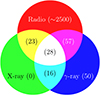 |
Fig. 7. Venn diagram of the normal pulsar population showing their repartition in different wavelengths: radio-only in red, X-ray-only in green, and γ-ray-only in blue. Other colours mean counts that the pulsars detected in at least two of these wavelengths. |
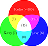 |
Fig. 8. Same as Fig. 7 but for millisecond pulsars. The question mark indicates that it was not possible to count these pulsars. No meaningful counts for X-ray-only or radio-loud X-ray pulsars were found; these are each indicated with a question mark (?). |
Statistics of 297 γ-ray pulsars detected by Fermi/LAT.
5.1. Radio-γ-ray population study
Our aim is to check whether the detected γ-ray pulsar distribution is compatible with an isotropic or uniform distribution of magnetic obliquity, χ, and line-of-sight inclination angle, ζ, assuming a striped wind model for γ-rays and a polar cap model for the radio band. To this end, we performed Monte-Carlo simulations, throwing ten million random numbers, Z, uniformly distributed in the interval [0, 1] for each angle, χ ∈ [0,π] and ζ ∈ [0, π]. The isotropic angle distribution depicted by the random variable, Θ, was then deduced by the change in the variable
 (23)
(23)
where Θ ∈ [0, π] is meant for either χ or ζ. The probability density function (p.d.f.) of both angles therefore follows a sin law according to
![Mathematical equation: $$ \begin{aligned} p(\Theta = \theta ) = \frac{\sin \theta }{2} ; \quad \theta \in [0,\pi ] . \end{aligned} $$](/articles/aa/full_html/2024/07/aa48069-23/aa48069-23-eq31.gif) (24)
(24)
For a uniform distribution of obliquities, we chose an angle from the distribution
 (25)
(25)
the angle, ζ, remaining isotropic. This distribution would mimic a tendency towards alignment of the pulsar obliquity. First, we compared the distribution of the γ-ray peak separation, Δ, given by Smith et al. (2023) to our simulated sample, knowing that a simple relation exists between Δ, χ, and ζ, given by Pétri (2011) as
 (26)
(26)
Our algorithm is therefore straightforward. We threw ten million instances of χ and, independently, ten million instances of ζ from an isotropic or a uniform distribution in χ and deduced Δ from Eq. (26). We restricted the separation to the interval Δ ∈ [0, 0.5]. If the observed Δ was larger than 0.5, we computed 1 − Δ, because Δ > 0.5 can be interpreted as Δ < 0.5 if the order of the γ-ray peaks is inverted. Applying this transformation, the results are summarised in the histogram of Fig. 9 showing the p.d.f.. The observations are depicted by green rectangles, whereas the simulated samples are depicted by orange rectangles for an isotropic χ distribution and blue rectangles for a uniform χ distribution. The agreement is satisfactory, although we overestimated slightly the probability of a separation close to half a period, Δ ≈ 0.5, in both cases. A uniform distribution gives however slightly better results.
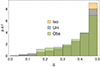 |
Fig. 9. γ-ray peak separation p.d.f. obtained from the observations (Obs) of 3PC in green vs. the model prediction for an isotropic (Iso) obliquity distribution in orange and a uniform (Uni) distribution in blue. |
In a previous work, Pétri & Mitra (2021) showed that the γ-ray lag, δ, is related to the peak separation, Δ, by an approximate relation such as
 (27)
(27)
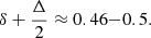
For high line-of-sight inclinations, it becomes closer to 0.46. We checked if this relation is satisfied in the 3PC pulsar catalogue, for young and millisecond pulsars independently. The results are shown in the histograms of Fig. 10. For the young pulsar population, we observe a strong peak in the range of 0.25 − 0.5, and thus a time lag of about 0.1 less in phase than the one predicted by the force-free model. There is a systematic effect that is missed in our description. This shift has already been noticed by Pétri (2011). The millisecond pulsars show a similar trend but are less peaked around 0.25 − 0.5 and the values are more spread between 0.1 and 0.8. We do not expect millisecond pulsars to sharply follow Eq. (27) because this formula assumes a dipolar field in the radio emission region, which is not the case for this population. The NICER collaboration found hotspots far from a geometry for a centred dipole. Off-centred or even multipole components are favoured, as was found by the studies of Riley et al. (2019) and Salmi et al. (2022). Moreover, Rigoselli & Mereghetti (2018) found absorption lines in the spectrum of PSR B1133+16, interpreted as proton cyclotron features, which thus implies multipolar components at the stellar surface. Other hints are given by Schwope et al. (2022) for J0659+1414, showing a complex variation in surface temperature that is also suggestive of the presence of a multipolar field.
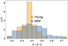 |
Fig. 10. Relation between time lag δ and peak separation Δ as given by Eq. (27) shown for the sample of young and millisecond pulsars from 3PC. |
This discrepancy can be explained by the fact that the high-energy radiation is not directed radially forward but is subject to a beaming in the direction of corotation that is not included in our striped wind model. We show how this proceeds by assuming particles moving at the speed of light along magnetic field lines in the equatorial plane for an orthogonal rotator. The particle velocity is β = Ω ∧ r + α t, where t is the unit vector tangent to the local field line. The angle between the radial direction and t is denoted by θ; thus, cos θ = er ⋅ t. Introducing a local planar Cartesian coordinate system (O, x, y) with the origin, O, at the light cylinder where emission starts, the speed is β2 = α2 − 2 α sin θ + 1. For ultra-relativistic speeds, β ≲ 1 and α = 0 or α = 2 sin θ. The first solution must be rejected because it corresponds to a straight line but the field line as swept back. Thus, the second solution applies. The angle, ϕ, between the particle velocity and the radial direction (the x axis) becomes tanϕ = vy/vx = cot(2 θ). The solution, therefore, is simply
 (28)
(28)
The angle, ϕ, introduces an additional time lag between radio waves and γ-rays of ϕ/(2π) in phase. Observations require this to be around 0.1; thus, ϕ ≈ π/5 and the magnetic field sweep-back angle is θ ≈ 3π/20 = 27°. We conclude that the magnetic field line must bend counter-clockwise at 27° to account for this additional shift. This value is compatible with a force-free neutron star magnetosphere. Variation in the bending leads to a spread in the time lag. In order to check this idea in the general case, we computed new γ-ray light curves by orienting the velocity vector in the forward direction with an inclination of 45° with respect to the radial direction. The quantity δ + Δ/2 is shown in Fig. 11, where it ranges from 0.32 to 0.42, which corresponds to the peak in the histogram of Fig. 10. With a non-radial flow, the agreement between observations and our model improves. The fact that the particle velocity right outside the light cylinder must be non-radial was already noticed by Contopoulos et al. (2020), who found a decreasing azimuthal component and an increasing radial component.
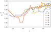 |
Fig. 11. Quantity δ + Δ/2 for the pulsar wind particle velocity oriented in the forward direction with an angle of 45° with respect to the radial direction. |
Next, we investigated the proportion of radio-loud and radio-quiet γ-ray pulsars as well as γ-quiet pulsars. In order to decide whether a pulsar would be seen in γ-rays or not, we computed the quantity G = χ−|ζ−π/2| from Eq. (8). A positive value of G means that the pulsar is visible in γ-rays. Figure A.8 shows the p.d.f. of this quantity, G. By construction, the total area of this histogram equals unity and the area delimited by G > 0 corresponds to the probability of detecting a γ-ray pulsar. We find that this area is equal to 0.89; therefore, 89% of the pulsar population should be seen as γ-ray pulsars.
Figure 12 shows the fraction of radio-only pulsars, γ-only pulsars, and radio-loud γ-ray pulsars as a function of the radio beam cone half-opening angle, ρ. The solid line represents the results for an isotropic χ, whereas the dashed line represents them for a uniform χ. Figure 13 shows the evolution of the fraction of radio-loud γ-ray pulsars with one peak, two peaks, and invisible pulsars (not detected in either radio or γ) as a function of ρ. For a beam angle of ρ ≈ 25°, half of the γ-ray pulsars are detected in radio. Table 2 summarises the simulated pulsar population for isotropic and uniform obliquity distributions at different wavelengths. New γ-ray pulsars are still being discovered in unassociated Fermi-LAT sources by recent surveys, like for instance the Transients and Pulsars with MeerKAT (TRAPUM) Large Survey Project (Clark et al. 2023) or the Einstein@Home blind search survey (Wu et al. 2018). There also exist several thousand unidentified γ-ray sources in the Fermi catalogue. A significant fraction could be pulsars and the statistics discussed in this work could evolve in the future.
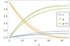 |
Fig. 12. Fraction of radio-only pulsars (r), γ-only pulsars (γ), and radio-loud γ-ray pulsars (γ + r) as a function of the radio beam cone half-opening angle, ρ. The solid line represents the results for an isotropic χ, whereas the dashed line represents them for a uniform χ. |
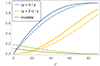 |
Fig. 13. Fraction of radio-loud γ-ray pulsars with one peak (γ + r)/γ and two peaks (γ + 2r)/γ and fraction of invisible pulsars (not detected in either r or γ). The solid line represents isotropic χ and the dashed line uniform χ. |
Summary of simulated pulsar population for isotropic and uniform obliquity distributions.
A similar study can be conducted for the radio loudness. The relevant quantities are N = |ζ − χ| and S = |ζ + χ − π|, according to Eqs. (9) and (10). In fact, the condition N ≤ ρ is sufficient because both p.d.f.s are almost identical. Figure A.7 shows the p.d.f. of N only as this is sufficient to decide whether a pulsar will be seen in radio or not. To complete, we need to fix the radio beam cone opening angle, ρ. The beam size depends on the pulsar period and on the emission height. For young pulsars, this height is constrained to lie around h ≈ 0.03 − 0.1 rL, according to Mitra (2017) and to compiled data from Weltevrede & Johnston (2008).
The period distribution of the millisecond and young pulsar show a bi-modal shape well separated and sharply peaked around a mean value. The mean and median values are summarised in Table 3. A typical young pulsar period is P = 150 ms. The cone opening angle is therefore of the order
 (29)
(29)
Mean and median period of MSP and young pulsars in the Fermi catalogue.
From Table 1, we conclude that 85/151 ≈ 56% of the young γ-ray pulsars are detected in radio. To get this percentage requires ρ ≈ 24 − 28°. This would correspond to an average emission height of 8–11% of rL. For the millisecond pulsars (MSP), 140/146 ≈ 95% are detected as radio pulsars; almost all the population of MSP. This is due to the fact that the radio beam cone is much wider compared to young pulsars. This percentage requires a cone opening angle of ρ ≈ 108° associated with an average emission height equal to a significant fraction of rL. In this case, the magnetic field has significant multipolar components and the expression for the cone width fails. We cannot infer any height for the radio emission, except that it is produced within the light cylinder, at a significant fraction of rL.
Pulse width comparisons are another important check for the radio modelling. We used the data from Posselt et al. (2021). Figure 14 shows the results of our model for an isotropic distribution of magnetic obliquity χ, denoted by ‘Iso’, in orange, and a uniform distribution denoted by ‘Uni’, in blue, compared to the observations denoted by ‘Obs’, in green. For a better match between our model and the observations, we took a radio emission cone opening angle of ρem ≈ 16°, which is about 2/3 of the radio cone beam width, ρ ≈ 24°. We emphasise that these values are average quantities and that obviously all pulsars do not possess the same radio beam geometry, some being larger and some smaller than ρ ≈ 16°. This scattering leads to a larger spread in the pulse width histogram shown in Fig. 14. We advise the reader to consult for instance the work of Dirson et al. (2022) for such refinement, which is out of the scope of the present paper.
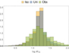 |
Fig. 14. Pulse width, W10, at 10% maximal height for an isotropic distribution of magnetic obliquity χ, denoted as ‘Iso’, in orange, and a uniform distribution denoted as ‘Uni’, in blue, compared to the observations denoted by ‘Obs’, in green. |
5.2. X-ray population study
The data about thermal and non-thermal X-ray emission from pulsars are more scarce. No detailed catalogue exists, such as those for radio or γ-rays. It is therefore difficult to get a precise idea of the population of X-ray pulsars, especially those showing pulsation in non-thermal X-rays. However, compiling data from Chang et al. (2023) and Coti Zelati et al. (2020) gives some hints about this particular population of pulsars. It is expected that more γ-ray sources and pulsar candidates will be associated with X-ray sources, as was revealed recently by Mayer & Becker (2024) with the SRG/eROSITA satellite. The census presented here therefore serves at most as a lower bound for the counting of pulsars shining in non-thermal X-rays. Orders of magnitude for the class of young and millisecond pulsars have been presented in Figs. 7 and 8.
To a first approximation, the population of X-ray pulsars follows the same trend as the radio pulsars because the emission geometries built onto a magnetic dipole, if well inside the light cylinder, are very similar. The highest emission altitude determines the fraction of the sky illuminated by X-rays, and therefore the fraction of pulsars detected in X-ray in addition to radio and/or γ-rays. Consequently, we can use the same Figs. 12 and 13 to deduce the expected number of detections in pulsed X-ray. The opening angle of the X-ray beam is much wider than the radio beam, leading to a large fraction of pulsars seen simultaneously in X-ray and γ-rays. But this hypothesis cannot be tested with high confidence because of the lack of an exhaustive census of X-ray pulsations.
Millisecond pulsars are difficult to fit into the picture of a dipolar field structure in the emission region. We therefore limited the X-ray expectations to the young non-recycled pulsar population. The number of X-ray visible γ-ray pulsars is 44 for a total number of 151 γ-ray pulsars, and thus a fraction of 44/151 ≈ 0.29 = 29% of X-ray loud γ-ray pulsars. This would correspond to an X-ray beam opening angle of ρX ≈ 15° and a low emission height along the separatrix, close to the radio emission site. We suspect that many pulsars should be detected in X-ray but the current low statistics do not allow us to put reliable constraints on the non-thermal X-ray emission so far.
In order to reliably test the X-ray emission model in the current state, a different approach must be undertaken. One possibility is to resort to the fitting of individual pulsar X-ray light curves, using geometrical constraints obtained from radio and γ-ray profile fitting, as was done by Benli et al. (2021) and Pétri & Mitra (2021). Young pulsars are the best targets because of the dominant dipole field in the emission regions. Good candidates are therefore γ-ray pulsars from the 3PC, seen simultaneously pulsating in radio and X-ray. However, such a study goes far beyond the scope of this paper, which is intended only to study pulsars as a population, not individually.
6. Conclusions
Radio as well as γ-ray emission regions are well constrained to be located above the polar caps for the former and in the current sheet of the striped wind for the latter. Nevertheless, the origin of the non-thermal X-ray radiation is less well established and only very few, if any, reliable constraints have been settled with high confidence. The comprehensive set of multi-wavelength pulse profiles computed in this work serves as an efficient and powerful tool with which to investigate and localise the X-ray photon production site by jointly fitting the radio pulse profile, the γ-ray light curve, and the non-thermal X-rays. As an application of the present work, in a subsequent paper, we will apply this fitting technique to several radio-loud X- and γ-ray pulsars and show how to reliably localise the non-thermal X-rays, like for instance those of PSR J2229+6114, a pulsar bright enough in X-rays. Moreover, based on the third pulsar catalogue, we have been able to estimate an average radio emission altitude. We show that the pulsar sub-populations of young and millisecond pulsars are compatible with an isotropic distribution of magnetic obliquity and line-of-sight inclination angles, although an evolution towards alignment is not excluded by our study.
This work is entirely based on geometrical effects to compute the light curves. No mention has been made of the energetics and dynamics of the charged particles evolving in this electromagnetic field, and only some guesses are provided. As the force-free model cannot accelerate particles, it is difficult to estimate the Lorentz factor and the radiation energy output of this model. A good compromise between the ideal force-free flow and the fully kinetic description of the magnetosphere would be to investigate the resistive regime, allowing for a substantial parallel electric field able to accelerate particles to ultra-relativistic energies. The multi-wavelength light curves would then depend on a new independent parameter depicting a kind of resistivity if an Ohm’s law is employed. This is left to a future work.
Acknowledgments
I am grateful to the referee for helpful comments and suggestions that improved the quality of the paper. I would like to thank David Smith for stimulating discussions. This work has been supported by the CEFIPRA grant IFC/F5904-B/2018 and ANR-20-CE31-0010.
References
- Arendt, P. N., Jr, & Eilek, J. A. 2002, ApJ, 581, 451 [NASA ADS] [CrossRef] [Google Scholar]
- Benli, O., Pétri, J., & Mitra, D. 2021, A&A, 647, A101 [NASA ADS] [CrossRef] [EDP Sciences] [Google Scholar]
- Beskin, V. S., Gurevich, A. V., & Istomin, Y. N. 1993, Physics of the Pulsar Magnetosphere (Cambridge: Cambridge University Press) [Google Scholar]
- Blaskiewicz, M., Cordes, J. M., & Wasserman, I. 1991, ApJ, 370, 643 [Google Scholar]
- Brambilla, G., Kalapotharakos, C., Harding, A. K., & Kazanas, D. 2015, ApJ, 804, 84 [NASA ADS] [CrossRef] [Google Scholar]
- Brambilla, G., Kalapotharakos, C., Timokhin, A. N., Harding, A. K., & Kazanas, D. 2018, ApJ, 858, 81 [NASA ADS] [CrossRef] [Google Scholar]
- Cerutti, B., & Philippov, A. A. 2017, A&A, 607, A134 [NASA ADS] [CrossRef] [EDP Sciences] [Google Scholar]
- Cerutti, B., Mortier, J., & Philippov, A. A. 2016a, MNRAS, 463, L89 [NASA ADS] [CrossRef] [Google Scholar]
- Cerutti, B., Philippov, A. A., & Spitkovsky, A. 2016b, MNRAS, 457, 2401 [Google Scholar]
- Cerutti, B., Philippov, A. A., & Dubus, G. 2020, A&A, 642, A204 [NASA ADS] [CrossRef] [EDP Sciences] [Google Scholar]
- Chang, H.-K., Hsiang, J.-Y., Chu, C.-Y., et al. 2023, MNRAS, 520, 4068 [NASA ADS] [CrossRef] [Google Scholar]
- Chen, J. L., & Wang, H. G. 2014, ApJS, 215, 11 [NASA ADS] [CrossRef] [Google Scholar]
- Clark, C. J., Breton, R. P., Barr, E. D., et al. 2023, MNRAS, 519, 5590 [NASA ADS] [CrossRef] [Google Scholar]
- Contopoulos, I., Kazanas, D., & Fendt, C. 1999, ApJ, 511, 351 [Google Scholar]
- Contopoulos, I., Pétri, J., & Stefanou, P. 2020, MNRAS, 491, 5579 [NASA ADS] [CrossRef] [Google Scholar]
- Coti Zelati, F., Torres, D. F., Li, J., & Viganó, D. 2020, MNRAS, 492, 1025 [NASA ADS] [CrossRef] [Google Scholar]
- Dirson, L., Pétri, J., & Mitra, D. 2022, A&A, 667, A82 [NASA ADS] [CrossRef] [EDP Sciences] [Google Scholar]
- Dyks, J., & Rudak, B. 2003, ApJ, 598, 1201 [NASA ADS] [CrossRef] [Google Scholar]
- Dyks, J., Harding, A. K., & Rudak, B. 2004, ApJ, 606, 1125 [Google Scholar]
- Gil, J., Melikidze, G. I., & Geppert, U. 2003, A&A, 407, 315 [NASA ADS] [CrossRef] [EDP Sciences] [Google Scholar]
- Harding, A. K. 2016, J. Plasma Phys., 82, 635820306 [CrossRef] [Google Scholar]
- Harding, A. K., DeCesar, M. E., Miller, M. C., Kalapotharakos, C., & Contopoulos, I. 2011, Fermi Symposium proceedings, eConf C110509 [Google Scholar]
- Íñiguez Pascual, D., Viganó, D., & Torres, D. F. 2022, MNRAS, 516, 2475 [CrossRef] [Google Scholar]
- Johnston, S., & Karastergiou, A. 2019, MNRAS, 485, 640 [NASA ADS] [CrossRef] [Google Scholar]
- Johnston, S., & Kramer, M. 2019, MNRAS, 490, 4565 [NASA ADS] [CrossRef] [Google Scholar]
- Johnston, S., Karastergiou, A., Mitra, D., & Gupta, Y. 2008, MNRAS, 388, 261 [NASA ADS] [CrossRef] [Google Scholar]
- Johnson, T. J., Venter, C., Harding, A. K., et al. 2014, ApJS, 213, 6 [Google Scholar]
- Johnston, S., Kramer, M., Karastergiou, A., et al. 2023, MNRAS, 520, 4801 [Google Scholar]
- Kalapotharakos, C., Kazanas, D., Harding, A., & Contopoulos, I. 2012, ApJ, 749, 2 [NASA ADS] [CrossRef] [Google Scholar]
- Kalapotharakos, C., Harding, A. K., Kazanas, D., & Brambilla, G. 2017, ApJ, 842, 80 [NASA ADS] [CrossRef] [Google Scholar]
- Kalapotharakos, C., Brambilla, G., Timokhin, A., Harding, A. K., & Kazanas, D. 2018, ApJ, 857, 44 [NASA ADS] [CrossRef] [Google Scholar]
- Kalapotharakos, C., Wadiasingh, Z., Harding, A. K., & Kazanas, D. 2023, ApJ, 954, 204 [NASA ADS] [CrossRef] [Google Scholar]
- Kazbegi, A. Z., Machabeli, G. Z., & Melikidze, G. I. 1991, MNRAS, 253, 377 [CrossRef] [Google Scholar]
- Kirk, J. G., Skjæraasen, O., & Gallant, Y. A. 2002, A&A, 388, L29 [NASA ADS] [CrossRef] [EDP Sciences] [Google Scholar]
- Kisaka, S., & Tanaka, S. J. 2014, MNRAS, 443, 2063 [NASA ADS] [CrossRef] [Google Scholar]
- Kisaka, S., & Tanaka, S. J. 2017, ApJ, 837, 76 [NASA ADS] [CrossRef] [Google Scholar]
- Kuiper, L., & Hermsen, W. 2015, MNRAS, 449, 3827 [NASA ADS] [CrossRef] [Google Scholar]
- Manchester, R. N., Hobbs, G. B., Teoh, A., & Hobbs, M. 2005, AJ, 129, 1993 [Google Scholar]
- Mayer, M. G. F., & Becker, W. 2024, A&A, 684, A208 [NASA ADS] [CrossRef] [EDP Sciences] [Google Scholar]
- Mitra, D. 2017, JApA, 38, 52 [NASA ADS] [Google Scholar]
- Noutsos, A., Sobey, C., Kondratiev, V. I., et al. 2015, A&A, 576, A62 [NASA ADS] [CrossRef] [EDP Sciences] [Google Scholar]
- Orens, J. H., Young, T., Oran, E., & Coffey, T. 1979, Vector Operations in a Dipole Coordinate System, Tech. Rep. NRL Memo. Rep. 3984, Naval Research Laboratory, Washington, D.C. [Google Scholar]
- Peng, Q.-Y., & Zhang, L. 2008, PASJ, 60, 771 [NASA ADS] [CrossRef] [Google Scholar]
- Pétri, J. 2011, MNRAS, 412, 1870 [Google Scholar]
- Pétri, J. 2012, MNRAS, 424, 605 [Google Scholar]
- Pétri, J. 2018, MNRAS, 477, 1035 [Google Scholar]
- Pétri, J. 2022a, MNRAS, 512, 2854 [CrossRef] [Google Scholar]
- Pétri, J. 2022b, A&A, 659, A147 [NASA ADS] [CrossRef] [EDP Sciences] [Google Scholar]
- Pétri, J., & Mitra, D. 2021, A&A, 654, A106 [NASA ADS] [CrossRef] [EDP Sciences] [Google Scholar]
- Philippov, A. A., Spitkovsky, A., & Cerutti, B. 2015, ApJ, 801, L19 [NASA ADS] [CrossRef] [Google Scholar]
- Phillips, J. A. 1992, ApJ, 385, 282 [NASA ADS] [CrossRef] [Google Scholar]
- Pierbattista, M., Harding, A. K., Grenier, I. A., et al. 2015, A&A, 575, A3 [NASA ADS] [CrossRef] [EDP Sciences] [Google Scholar]
- Pierbattista, M., Harding, A. K., Gonthier, P. L., & Grenier, I. A. 2016, A&A, 588, A137 [NASA ADS] [CrossRef] [EDP Sciences] [Google Scholar]
- Posselt, B., Karastergiou, A., Johnston, S., et al. 2021, MNRAS, 508, 4249 [NASA ADS] [CrossRef] [Google Scholar]
- Rigoselli, M., & Mereghetti, S. 2018, A&A, 615, A73 [NASA ADS] [CrossRef] [EDP Sciences] [Google Scholar]
- Riley, T. E., Watts, A. L., Bogdanov, S., et al. 2019, ApJ, 887, L21 [Google Scholar]
- Salmi, T., Vinciguerra, S., Choudhury, D., et al. 2022, ApJ, 941, 150 [CrossRef] [Google Scholar]
- Schwope, A., Pires, A. M., Kurpas, J., et al. 2022, A&A, 661, A41 [NASA ADS] [CrossRef] [EDP Sciences] [Google Scholar]
- Smith, D. A., Abdollahi, S., Ajello, M., et al. 2023, ApJ, 958, 191 [NASA ADS] [CrossRef] [Google Scholar]
- Spitkovsky, A. 2006, ApJ, 648, L51 [Google Scholar]
- Swisdak, M. 2006, arXiv e-prints [arXiv:physics/0606044] [Google Scholar]
- Takata, J., & Cheng, K. S. 2017, ApJ, 834, 4 [NASA ADS] [CrossRef] [Google Scholar]
- Timokhin, A. N., & Harding, A. K. 2019, ApJ, 871, 12 [NASA ADS] [CrossRef] [Google Scholar]
- Torres, D. F., Viganò, D., Coti Zelati, F., & Li, J. 2019, MNRAS, 489, 5494 [NASA ADS] [CrossRef] [Google Scholar]
- Usov, V. V. 2002, Proceedings of the 270 WE-Heraeus Seminar on Neutron Stars, Pulsars, and Supernova Remnants, MPE Report 278, eds. W. Becker, H. Lesch, & J. Trümper (Garching bei München: Max-Plank-Institut für extraterrestrische Physik), 240 [Google Scholar]
- Venter, C., Harding, A. K., & Grenier, I. 2018, in Proceedings of XII Multifrequency Behaviour of High Energy Cosmic Sources Workshop, eds. F. Giovannelli, & L. Sabau-Graziati, PoS(MULTIF2017), 306, 38 [Google Scholar]
- Watters, K. P., Romani, R. W., Weltevrede, P., & Johnston, S. 2009, ApJ, 695, 1289 [Google Scholar]
- Weltevrede, P., & Johnston, S. 2008, MNRAS, 391, 1210 [NASA ADS] [CrossRef] [Google Scholar]
- Wu, J., Clark, C. J., Pletsch, H. J., et al. 2018, ApJ, 854, 99 [Google Scholar]
- Zhang, L., & Jiang, Z. J. 2006, A&A, 454, 537 [NASA ADS] [CrossRef] [EDP Sciences] [Google Scholar]
Appendix A: Multi-wavelength atlas
In this appendix, we present several atlases of light curves in radio, X-ray, and γ-ray. Fig. A.1 shows a sample of typical radio pulse profiles when the emission height is set in the range r/rL ∈ [0.1, 0.11]. Two radio pulses are observed for almost orthogonal rotators, as was expected. In these plots, even if the line of sight does not intersect the radio cone, we plot the pulse profiles, corresponding to the bottom left and top right of the figure. The radio duty cycles appear therefore to be artificially wider because the radio visibility condition (eq. (9) or eq. (10)) is not met. Fig. A.2 shows the γ-ray light curves for different emission intervals, in blue for the range r/rL ∈ [1, 2], in green for the range r/rL ∈ [2, 3], and in red for the total interval, r/rL ∈ [1, 3]. We observe a slight change in the profile shapes around the values satisfying χ + ζ ≈ π/2, corresponding to the line of sight grazing the current sheet. In all other geometries, the profile is insensitive to the distance. Two examples of X-ray light curves are shown in fig. A.3 for an emission height in the range r/rL ∈ [0.1, 0.2] and fig. A.4 for an emission height in the range r/rL ∈ [0.4, 0.5]. As the extension of the emission region in X-ray is unconstrained, we plotted the effect of stacking together several adjacent emission sites to obtain a set of possible pulse profiles, as is shown in fig A.5 for an obliquity of χ = 45° and a line-of-sight inclination of ζ = 44°. Single and double peak structures are obtained with a symmetric or an asymmetric shape. Such profiles must be fitted to individual pulsars to extract useful information about the X-ray emission mechanisms. Collecting the radio, X-ray, and γ-ray pulse profiles, figure A.6 shows the multi-wavelength light curves for an obliquity of χ = 15° and line-of-sight inclinations of ζ = {10° ,30° ,50° ,70° ,90° } with the legend format {χ,ζ,em}, where em can be r for radio, X for X-rays, or γ for γ-rays, in solid red, green, and blue lines, respectively, in the first, second, and third rows. Other examples for χ = 45° and χ = 75° are also shown in the same figure ( A.6, middle panels and bottom panels, respectively).
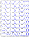 |
Fig. A.1. Atlas of radio pulse profile for photons produced in the range r/rL ∈ [0.1, 0.11]. The geometry is shown in the inset as brackets {χ,ζ}. |
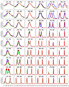 |
Fig. A.2. Atlas of γ-ray light curves when emission emanates from the range r/rL ∈ [1, 2] in blue, in the range r/rL ∈ [2, 3] in green, and the total r/rL ∈ [1, 3] in red. The geometry is shown in the inset as brackets {χ,ζ}. |
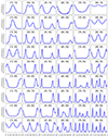 |
Fig. A.3. Atlas of X-ray light curves when emission emanates from the range r/rL ∈ [0.1, 0.2]. The geometry is shown in the inset as brackets ({χ,ζ}). |
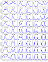 |
Fig. A.4. Atlas of X-ray light curves when emission emanates from the range r/rL ∈ [0.4, 0.5]. The geometry is shown in the inset as brackets {χ,ζ}. |
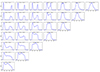 |
Fig. A.5. Evolution of the X-ray profile with altitude and extension of the emission region for χ = 45° and ζ = 44°. The legend shows the lower and upper radii, {rin/rL, rout/rL}, respectively denoted by rin and rout, for the region of the separatrix emitting in X-ray. The upper rows show the individual light curves that are progressively added together in the lower rows to the point where all are stacked to get only one possible light curve, shown by the lowest row. |
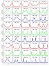 |
Fig. A.6. Multi-wavelength light curves for χ = 15° in the top panel, χ = 45° in the middle panel, and χ = 75° in the bottom panel, with ζ = {10° ,30° ,50° ,70° ,90° }. The legend is {χ,ζ,em}, where em stands for the three energy bands as r for radio (red), X for X-rays (green), or γ for γ-rays (blue). |
To decide whether a pulsar is visible in radio or γ-ray, we plotted the p.d.f. for N in fig. A.7 and for G in fig. A.8 for an isotropic and uniform distribution of magnetic obliquities, in orange and blue, respectively.
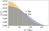 |
Fig. A.7. Probability density function of N to decide for the pulsar radio visibility, isotropic (Iso) obliquity distribution in orange and uniform (Uni) distribution in blue. The fraction of radio pulsars detected depends on the radio beam half-opening angle ρ. |
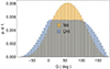 |
Fig. A.8. Probability density function of G to decide whether the pulsar is visible in γ-ray or not, isotropic (Iso) obliquity distribution in orange and uniform (Uni) distribution in blue. The region G > 0 separates the pulsars visible in γ-ray from those invisible G < 0. G is given in degrees (deg). |
Appendix B: Dipolar coordinate system
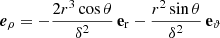
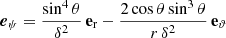
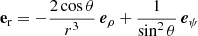
Around a star whose field close to the surface is essentially dipolar, it is useful to choose a coordinate system, following the geometry of the magnetic field lines. Starting from the spherical polar coordinates (r, θ, ϕ) with a natural basis (er, eθ, eϕ), we introduce the new coordinates (ρ, ψ, ϕ) and an associated natural basis (eρ, eψ, eϕ) defined by
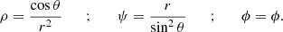 (B.1)
(B.1)
The spherical radius, r, is found implicitly by solving the fourth-order polynomial
 (B.2)
(B.2)
and the angle according to cos θ = ρ r2. The coordinate system is shown in a meridional plane in fig. B.1. The determinant of the Jacobian matrix,
 (B.3)
(B.3)
 |
Fig. B.1. Dipolar curvilinear coordinate system showing lines of constant ψ (red lines) and lines of constant ρ (blue lines). These coordinates are orthogonal. |
is
 (B.4)
(B.4)
with 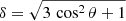 . The vectors of the natural basis are
 (B.5a)
 (B.5b)
and the inverse relations
 (B.6a)
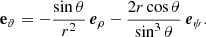 (B.6b)
This basis is orthogonal and the metric gik diagonal with
 (B.7a)
 (B.7b)
 (B.7c)
the surface element is
 (B.8)
(B.8)
and the volume element
 (B.9)
(B.9)
Finally, defining the orthonormal basis relations between  and
and  , we get
 (B.10a)
 (B.10b)
 (B.10c)
Particle are obliged to move along field lines defined by the separatrix surface. This corresponds to a motion with a fixed value for ψ and ϕ. This means that they move along the direction given by ∂/∂ρ, and thus along the unit vector,  . Photons are emitted in the radially outward direction, t, such that
  , implying that
 (B.11)
For the aligned rotator, the separatrix is defined by rsep = rL sin2θ and emission starts at an altitude of he; thus,  . A photon emitted at the position (re, θe, ϕe) will propagate in a direction with colatitude θx such that cos θx = tz = t ⋅ ez. Explicitly, we find
 (B.12)
Photons are produced between an emission height of h1 and h2 > h1. The observer will therefore detect X-rays if his line of sight, ζ, lies in the range spanned by the photon emission angle, θx; that is, ![Mathematical equation: $ \zeta \in [\theta_{\rm x}^1,\theta_{\rm x}^2] $](/articles/aa/full_html/2024/07/aa48069-23/aa48069-23-eq61.gif) , with
, with
 (B.13)
For an oblique dipole, we followed the same reasoning and rotated the Cartesian coordinate system to align the new z axis with the magnetic moment axis, and thus perform a rotation of angle, χ, along the x axis with the rotation matrix
 (B.14)
The photon propagation direction in the upper hemisphere case becomes
 (B.15)
The z component is
 (B.16)
The lower and upper bounds for this component are
 (B.17a)
 (B.17b)
Consequently, the photon emission direction when starting at position θe for an oblique rotator with obliquity χ stays between the two extremal values,
 (B.18)
This formula was expected, since the X-ray half-opening angle is θx and the cone is centred around the magnetic axis. This definition is exactly the same as for the radio emission cone opening angle; namely,
 (B.19)
The X-ray visibility will therefore mimic the radio visibility condition, the only difference being the size of the emitting cone because of the varying emission altitude postulated in X-rays. We emphasise that this view is correct for a static dipole, and thus restricted to altitudes of at most a fraction of the light cylinder. High altitude emission will significantly deviate from the above guess.
All Tables
Summary of simulated pulsar population for isotropic and uniform obliquity distributions.
All Figures
|
Fig. 1. Magnetic field lines in the equatorial plane for an orthogonal rotator with R/rL = 0.1. The neutron star is shown as a black disk and the light cylinder as a dashed black circle. |
| In the text | |
|
Fig. 2. Geometry showing the region of radio and γ-ray visibility depending on the magnetic obliquity, χ, and line of sight, ζ. The red area corresponds to γ-ray-only, the blue area to radio-only with ρ = 20°, and the magenta area to radio-loud γ-ray visibility. Due to the symmetry of the plot, the three other quadrants with χ ≥ π/2 or ζ ≥ π/2 are not shown. |
| In the text | |
|
Fig. 3. Map of radio, X-ray, and γ-ray radiation for different emission altitudes and for χ = {15°,45°,75°}. The legend shows the wavelength, emission interval, and obliquity. Maximum intensities are normalized and colour-coded in the right legend. |
| In the text | |
|
Fig. 4. Curvature in units of 1/rL along the separatrix, starting from the surface going to the light cylinder and back to the surface for the vacuum field (VAC, in orange) and the force-free solution (FFE, in blue). Values are shown for an obliquity of χ = 75°. |
| In the text | |
|
Fig. 5. Curvature of the magnetic axis for the VAC and the FFE. Values are shown for an obliquity of χ = 75°. |
| In the text | |
|
Fig. 6. Angle between the local magnetic field at radius r for points on the central field line and the magnetic moment direction for the VAC and the FFE. Values are shown for an obliquity of χ = 75°. |
| In the text | |
|
Fig. 7. Venn diagram of the normal pulsar population showing their repartition in different wavelengths: radio-only in red, X-ray-only in green, and γ-ray-only in blue. Other colours mean counts that the pulsars detected in at least two of these wavelengths. |
| In the text | |
|
Fig. 8. Same as Fig. 7 but for millisecond pulsars. The question mark indicates that it was not possible to count these pulsars. No meaningful counts for X-ray-only or radio-loud X-ray pulsars were found; these are each indicated with a question mark (?). |
| In the text | |
|
Fig. 9. γ-ray peak separation p.d.f. obtained from the observations (Obs) of 3PC in green vs. the model prediction for an isotropic (Iso) obliquity distribution in orange and a uniform (Uni) distribution in blue. |
| In the text | |
|
Fig. 10. Relation between time lag δ and peak separation Δ as given by Eq. (27) shown for the sample of young and millisecond pulsars from 3PC. |
| In the text | |
|
Fig. 11. Quantity δ + Δ/2 for the pulsar wind particle velocity oriented in the forward direction with an angle of 45° with respect to the radial direction. |
| In the text | |
|
Fig. 12. Fraction of radio-only pulsars (r), γ-only pulsars (γ), and radio-loud γ-ray pulsars (γ + r) as a function of the radio beam cone half-opening angle, ρ. The solid line represents the results for an isotropic χ, whereas the dashed line represents them for a uniform χ. |
| In the text | |
|
Fig. 13. Fraction of radio-loud γ-ray pulsars with one peak (γ + r)/γ and two peaks (γ + 2r)/γ and fraction of invisible pulsars (not detected in either r or γ). The solid line represents isotropic χ and the dashed line uniform χ. |
| In the text | |
|
Fig. 14. Pulse width, W10, at 10% maximal height for an isotropic distribution of magnetic obliquity χ, denoted as ‘Iso’, in orange, and a uniform distribution denoted as ‘Uni’, in blue, compared to the observations denoted by ‘Obs’, in green. |
| In the text | |
|
Fig. A.1. Atlas of radio pulse profile for photons produced in the range r/rL ∈ [0.1, 0.11]. The geometry is shown in the inset as brackets {χ,ζ}. |
| In the text | |
|
Fig. A.2. Atlas of γ-ray light curves when emission emanates from the range r/rL ∈ [1, 2] in blue, in the range r/rL ∈ [2, 3] in green, and the total r/rL ∈ [1, 3] in red. The geometry is shown in the inset as brackets {χ,ζ}. |
| In the text | |
|
Fig. A.3. Atlas of X-ray light curves when emission emanates from the range r/rL ∈ [0.1, 0.2]. The geometry is shown in the inset as brackets ({χ,ζ}). |
| In the text | |
|
Fig. A.4. Atlas of X-ray light curves when emission emanates from the range r/rL ∈ [0.4, 0.5]. The geometry is shown in the inset as brackets {χ,ζ}. |
| In the text | |
|
Fig. A.5. Evolution of the X-ray profile with altitude and extension of the emission region for χ = 45° and ζ = 44°. The legend shows the lower and upper radii, {rin/rL, rout/rL}, respectively denoted by rin and rout, for the region of the separatrix emitting in X-ray. The upper rows show the individual light curves that are progressively added together in the lower rows to the point where all are stacked to get only one possible light curve, shown by the lowest row. |
| In the text | |
|
Fig. A.6. Multi-wavelength light curves for χ = 15° in the top panel, χ = 45° in the middle panel, and χ = 75° in the bottom panel, with ζ = {10° ,30° ,50° ,70° ,90° }. The legend is {χ,ζ,em}, where em stands for the three energy bands as r for radio (red), X for X-rays (green), or γ for γ-rays (blue). |
| In the text | |
|
Fig. A.7. Probability density function of N to decide for the pulsar radio visibility, isotropic (Iso) obliquity distribution in orange and uniform (Uni) distribution in blue. The fraction of radio pulsars detected depends on the radio beam half-opening angle ρ. |
| In the text | |
|
Fig. A.8. Probability density function of G to decide whether the pulsar is visible in γ-ray or not, isotropic (Iso) obliquity distribution in orange and uniform (Uni) distribution in blue. The region G > 0 separates the pulsars visible in γ-ray from those invisible G < 0. G is given in degrees (deg). |
| In the text | |
|
Fig. B.1. Dipolar curvilinear coordinate system showing lines of constant ψ (red lines) and lines of constant ρ (blue lines). These coordinates are orthogonal. |
| In the text | |
Current usage metrics show cumulative count of Article Views (full-text article views including HTML views, PDF and ePub downloads, according to the available data) and Abstracts Views on Vision4Press platform.
Data correspond to usage on the plateform after 2015. The current usage metrics is available 48-96 hours after online publication and is updated daily on week days.
Initial download of the metrics may take a while.