| Issue |
A&A
Volume 686, June 2024
|
|
|---|---|---|
| Article Number | A238 | |
| Number of page(s) | 8 | |
| Section | The Sun and the Heliosphere | |
| DOI | https://doi.org/10.1051/0004-6361/202450030 | |
| Published online | 14 June 2024 | |
Evolution of the magnetic field rotation distributions in the inner heliosphere
1
Istituto per la Scienza e la Tecnologia dei Plasmi, Consiglio Nazionale delle Ricerche, 70126 Bari, Italy
e-mail: This email address is being protected from spambots. You need JavaScript enabled to view it.
2
Department of Physics and Astronomy, Queen Mary University of London, London E1 4NS, UK
3
Johns Hopkins University Applied Physics Laboratory, Laurel, MD 20723, USA
4
Space and Plasma Physics, School of Electrical Engineering and Computer Science, KTH Royal Institute of Technology, 11428 Stockholm, Sweden
Received:
19
March
2024
Accepted:
19
April
2024
Abstract
Context. The nature and evolution of the solar wind magnetic field rotations is studied in data from the Parker Solar Probe.
Aims. We investigated the magnetic field deflections in the inner heliosphere below 0.5 au in a distance- and scale-dependent manner to shed some light on the mechanism behind their evolution.
Methods. We used the magnetic field data from the FIELDS instrument suite to study the evolution of the magnetic field vector increment and rotation distributions that contain switchbacks.
Results. We find that the rotation distributions evolve in a scale-dependent fashion. They have the same shape at small scales regardless of the radial distance, in contrast to larger scales, where the shape evolves with distance. The increments are shown to evolve towards a log-normal shape with increasing radial distance, even though the log-normal fit works quite well at all distances, especially at small scales. The rotation distributions are shown to evolve towards a previously developed rotation model moving away from the Sun.
Conclusions. Our results suggest a scenario in which the evolution of the rotation distributions is primarily the result of the expansion-driven growth of the fluctuations, which are reshaped into a log-normal distribution by the solar wind turbulence.
Key words: turbulence / Sun: corona / Sun: magnetic fields / solar wind
© The Authors 2024
 Open Access article, published by EDP Sciences, under the terms of the Creative Commons Attribution License (https://creativecommons.org/licenses/by/4.0), which permits unrestricted use, distribution, and reproduction in any medium, provided the original work is properly cited.
This article is published in open access under the Subscribe to Open model. This email address is being protected from spambots. You need JavaScript enabled to view it. to support open access publication.
1. Introduction
The solar wind is a turbulent medium whose properties evolve with radial distance from the Sun (Bruno & Carbone 2013). In recent years, data from the Parker Solar Probe (PSP) mission have provided an unparalleled opportunity to study fluctuations in the solar wind at unprecedentedly close distances to the Sun (Chen et al. 2020; Adhikari et al. 2020, 2022; Alberti et al. 2020; Zhu et al. 2020; Huang et al. 2021; Shi et al. 2021; D’Amicis et al. 2021; Hernández et al. 2021; Telloni et al. 2021; Zhao et al. 2022; Bandyopadhyay et al. 2022; Sioulas et al. 2023a; McIntyre et al. 2023; Cuesta et al. 2023; Bowen et al. 2024), see Raouafi et al. (2023) for a review. These observations, combined with high-resolution numerical simulations (Perez & Chandran 2013; Dong et al. 2014; Verdini & Grappin 2015; Pezzi et al. 2017; Chandran & Perez 2019; Ruffolo et al. 2020; Squire et al. 2020; Meyrand et al. 2021; Shi et al. 2023; Trotta et al. 2023; Sorriso-Valvo et al. 2023; Matteini et al. 2024), have greatly enhanced our understanding of the near-Sun solar wind turbulence.
A longstanding debate that PSP data can help solve is whether the large-amplitude rotations or discontinuities observed in the solar wind can be attributed to a turbulent phenomenology, or if a different picture has to be invoked. An alternative scenario is the spaghetti-like solar wind, in which discontinuities are interpreted as flux-tube walls crossed by the spacecraft (see Li 2008, and references therein).
Borovsky (2008) interpreted the possibility that the rotation distribution can be fit with a double-exponential function as an indication that two populations are present. A population of small rotations, below ≈30°, due to turbulence and another population with rotations above ≈50° indicative of the presence of flux tubes. Further support to this picture was given with the observation of changes in the plasma properties across discontinuities (Borovsky 2008, 2010, 2020). However, some plasma properties, such as the alpha-to-proton ratio, do not show a significant correlation with magnetic field rotations (Owens et al. 2011).
A different picture emerges from the work of Zhdankin et al. (2012), who reported a good agreement between the experimental rotation distributions at 1 au and simulations of MHD turbulence for many different scales within the inertial range. Furthermore, a different model for the rotation distributions was proposed. This model was based on the fact that the vector increment magnitude probability density functions (PDFs) at 1 au, computed at different time lags, have a log-normal shape. While the parameters of the log-normal distributions differ for each lag, the PDFs can be rescaled to a universal (i.e. scale-independent) log-normal distribution in the inertial range. From the universal log-normal, the rotation model was recovered. This picture is also supported by the agreement between proxies for magnetic discontinuities and intermittency (Greco et al. 2008), which is a fundamental property of turbulence.
Several studies of turbulence have focused on the distributions of rotation angles and magnetic vector increments (see, e.g., Perri et al. 2009; Greco & Perri 2014). At large scales, at 1 au, both distributions become scale-independent in the 1/f range (Matteini et al. 2018). This behaviour holds for both the fast and slow Alfvénic wind, but not for the non-Alfvénic slow wind, as evidenced using Helios data (Perrone et al. 2020). In both the inertial range and the kinetic range, the increment distributions are shown to have approximately log-normal shape and to be mostly due to pure rotations (i.e. without changes in the magnitude of the magnetic field; Zhdankin et al. 2012; Chen et al. 2015).
Log-normal distributions are observed in the solar wind not only for magnetic increments (Bruno et al. 2004), but also for the magnetic field magnitude (Burlaga 2001), for the scale-dependent energy dissipation rate (Zhdankin et al. 2016), and as models of the energy cascade rate distributions (Sorriso-Valvo et al. 1999) in the context of multiplicative random cascade models (Castaing et al. 1990). In these models, the non-conservative (intermittent) behaviour of the local energy dissipation rate is modelled through the multiplication of random variables drawn from the same distribution (Frisch 1995). The log-normal is one of the possible distributions choices, but it seems to be the most common distribution in the solar wind (Sorriso-Valvo et al. 1999, 2015; Zhdankin et al. 2012, 2016), and it is probably a consequence of dealing with intermittent turbulent signals. It should be noted that another possibility, not investigated here, is the normal inverse Gaussian function, which was tested for the increments of the Elsasser variables in the solar wind (Palacios Caicedo 2021).
The study of the rotation distributions is of even more interest due to the recent measurements of magnetic switchbacks in PSP data (Bale et al. 2019; Kasper et al. 2019; Dudok de Wit et al. 2020; Squire et al. 2020; Krasnoselskikh et al. 2020; Zank et al. 2020; Tenerani et al. 2021; Larosa et al. 2021; Pecora et al. 2022; Jagarlamudi et al. 2023; Huang et al. 2023a). The origins of these structures and whether they can be considered a different population with respect to the background solar wind turbulence are still unknown (Dudok de Wit et al. 2020; Raouafi et al. 2023).
We study the evolution of the magnetic increments and rotation distributions in the solar wind at different radial distances to the Sun using PSP data. We focus on the changes in shape of the distributions, on their universality and on the validity of the Zhdankin et al. (2012) rotational model closer to the Sun.
In Sect. 2 we describe the data set we used in this study, in Sect. 3 we report our results, and in Sect. 4 we discuss our conclusions.
2. Data and methods
We used data from the PSP fluxgate magnetometer MAG (Bale et al. 2016) at a cadence of four samples per cycle (around 0.22 s) and the electron pitch-angle distributions (ePAD) from the SPAN-e (Solar Probe ANalyzer for Electrons) instrument (Kasper et al. 2016; Whittlesey et al. 2020). The data in this study cover the fist 11 orbits of PSP at distances below 0.5 au.
In the dataset, transients such as coronal mass ejections (CMEs) were removed by eye, and the heliospheric current sheet (HCS) crossings were removed with the aid of the ePAD. CMEs were excluded because they are not part of the steady-state solar wind, and the HCS crossings were excluded because they are large-angle rotations related to the change in the heliospheric magnetic field polarity rather than to turbulence.
We computed the distributions of the magnetic field increments,
 (1)
(1)
and the corresponding angular rotations,
 (2)
(2)
Under the assumption of pure rotations between t + τ and t without a change in field magnitude, the angle and increments are related by ΔB/B = 2sin(Δθ/2) (Zhdankin et al. 2012). Each data point in the time series provides an increment value unless B(t + τ) or B(t) are data gaps. In this case, no increment value is obtained. With a data series of increments at a given τ and distance, we computed the corresponding distribution.
In the distributions, we considered values of ΔB/B and corresponding rotations only for increments up to 2. This upper limit was set by the fact that a rotation of 180° can give a maximum increment value of 2. Therefore, any value higher than 2 cannot be the result of a pure rotation. Applying this threshold has the effect of removing part of the tail of the distributions (the part due to highly compressive increments), but fewer than 0.6% of the pre-processed points (without HCS crossings and CMEs) are lost as a consequence.
3. Results
3.1. Evolution of the increments and rotation distributions with heliocentric distance
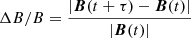
The evolution of the magnetic field increments with distance and scale is shown in Fig. 1. The different curves show evident variations with the heliocentric distance. For example, at small scales τ, the distribution closest to the Sun (blue line) presents the highest tail, indicating a higher probability of occurrence for large increments, whereas it has the lowest tails at large scales.
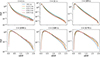 |
Fig. 1. Distributions of the magnetic field increments ΔB/B. The increments are computed at different timescales, τ, for each panel, as indicated at the top. The different colours represent different heliocentric distances. The shaded area represents the statistical error estimated as the square root of the number of points in a given bin. The error is not visible in most cases because it is small and comparable with the width of the plot lines. |
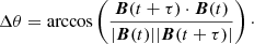
Figure 2 shows the rotation distributions. Not surprisingly, the curves behave similar to those of Fig. 1, since the magnetic field undergoes mostly rotation in the solar wind, especially at the distances of PSP. The dominance of the rotations is highlighted in Fig. 3, which shows the distribution of the parameter χ = |ΔB/B − 2sin(Δθ/2)|/(ΔB/B), a measure of the deviations from pure rotations. The distributions of χ are strongly peaked near zero, regardless of distance and scale, with a drop of more than 2 orders of magnitude between the peak value and the value at χ = 0.1. This confirms (see Zhdankin et al. 2012 for data at 1 au) the predominance of rotations in the solar wind also in the inner heliosphere.
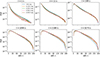 |
Fig. 2. Distributions of the magnetic deflection angles Δθ. The order of the panels and the meaning of the colours is the same as in Fig. 1. |
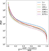 |
Fig. 3. Distributions of χ, the normalised difference between the magnetic vector increments and the corresponding angle if this were due to pure rotation. The different colors represent different values of τ. The solid lines are drawn at distances below 0.1 au, and the dotted lines are drawn at distances between 0.4 and 0.5 au. |
The behaviour of the PDFs in Figs. 1 and 2 is due in part to the fact that by using the same τ at different distances, we compare distributions with a different underlying average level of ΔB/B, and that we neglect the evolution of the 1/f break with distance (Bruno & Carbone 2013; Chen et al. 2020; Huang et al. 2023b; Davis et al. 2023). In order to clearly determine any changes in the shape of the distributions, we need to account for these effects. We did this by rescaling the timescales though the following procedure: (1) For each of the five distance classes used in Figs. 1 and 2, we computed the mean scale-dependent fluctuation level ⟨ΔB/B⟩, obtaining a set of empirical curves for ⟨ΔB/B⟩ against τ. (2) Based on these relations, we extrapolated for each distance the scales τ corresponding to a set of selected specific values of ⟨ΔB/B⟩, effectively rescaling all the fluctuations and angular increments to remove the radial evolution of ⟨ΔB/B⟩. (3) We used these values of ⟨ΔB/B⟩ as proxies for the scale, while the increments and the corresponding rotations were recomputed with the corresponding set of extrapolated timescales. The different values are reported in Table 1.
Values in seconds of the lag we used for different distances and different average values of ⟨ΔB/B⟩ to compute the increments.
The results are shown in Fig. 4, where the distributions of the rescaled rotations Δθ are shown for the different values of mean fluctuations ⟨ΔB/B⟩ (different panels), and for each distance to the Sun (different colours). At small ⟨ΔB/B⟩ (corresponding to small scales), the distributions collapse on the same shape for all distances. As the scale (or, equivalently, ⟨ΔB/B⟩) increases, the tails of the distribution increasingly separate, in particular, for short distance R < 0.1 au. This behaviour suggests that the small-scale distribution is already fully evolved at these distances, while at larger scales (⟨ΔB/B⟩> 0.1), it is still in the process of evolving to its final state. This scale dependence is highly suggestive of a turbulence-dominated PDF evolution because in a turbulent cascade the non-linear time is scale-dependent, with the smaller scales evolving faster.
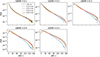 |
Fig. 4. Distributions of the magnetic deflection angles Δθ at fixed values of the average increment value ⟨ΔB/B⟩. |
3.2. Log-normality and the Zhdankin rotation model with PSP
In Fig. 5 we test whether the fluctuations ΔB/B follow a log-normal distribution throughout the full range of distances and scales considered here. The colours now refer to different scales, through the proxy ⟨ΔB/B⟩, according to the rescaling procedure described above, while different distances are represented in different panels. The log-normal distribution can be written as
![Mathematical equation: $$ \begin{aligned} f(x) = \frac{1}{x\sigma \sqrt{2\pi }} \exp \left[-\frac{1}{2}\left(\frac{\log {x}-\mu }{\sigma }\right)^{\!2}\,\right], \end{aligned} $$](/articles/aa/full_html/2024/06/aa50030-24/aa50030-24-eq3.gif) (3)
(3)
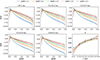 |
Fig. 5. Distributions of the magnetic field vector increments at fixed average ΔB/B. The dashed lines are log-normal fits to the data. The bottom right panel shows the variation with distance and scale of the parameter σ. |
where the parameters μ and σ represent the mean and standard deviation of log(x), respectively. The results in Fig. 5 clearly show that farther out in the heliosphere, the distributions are better fit by a log-normal, even though the fit is reasonably good even at the closest distances. In order to quantitatively evaluate the goodness of the log-normal fit, we computed the coefficient of determination defined as  , where yi and ⟨y⟩ are the measured values and their mean, respectively, fi represents the values of the model, and n the number of data points. The values of R vary from 0 to 1 as the goodness of fit increases. The coefficient of determination is close to 1 for all the cases in Fig. 5, indicating an excellent log-normal fit of the distributions. For ⟨ΔB/B⟩ = 0.5, corresponding to the largest scales used here, R increases from 0.90 at distances below 0.1 au to 0.97 at larger distances, in the range 0.4−0.5 au. For the smallest scales, corresponding to ⟨ΔB/B⟩ = 0.1, R = 0.98 at the closest distances indicates excellent agreement, which increases to R = 0.998 for the farthest distances. The bottom right panel of Fig. 5 illustrates the radial and scale-dependent evolution of the fitting parameter σ, which was found to be σ ≈ 1 at 1 au using Wind data (Zhdankin et al. 2012). We observe that σ increases with increasing radial distance for all scales (again represented by the different values of ⟨ΔB/B⟩). At large distance, the distributions seem to saturate to high values σ ≈ 1 for all scales, while at the closest distances, they show a larger spread, and the variance approaches the saturation value as the scale decreases. In particular, the variance increases form σ ≈ 0.79 for the largest-scale distributions (i.e. with ⟨ΔB/B⟩ = 0.5) to σ ≈ 0.85 for the smallest-scale distributions (⟨ΔB/B⟩ = 0.1).
We tested how other functions that are commonly used in the literature to describe the magnetic increments fit the PDFs in comparison with the log-normal function (not shown). A double exponential was used by Borovsky (2010) to fit the rotation angles Δθ, and it can be also tested for ΔB/B. This function has two additional fitting parameters with respect to the log-normal. It gives a determination coefficient very close to one only for smaller scales, with ⟨ΔB/B⟩ up to 0.3. For larger scales, the fits fail to converge. The reason is that the small ΔB/B downward section of the curve at ⟨ΔB/B⟩> 0.3 cannot be reproduced with a double exponential. The same is found when fitting Δθ. We also tested the log-Poisson distribution, which is observed for other measures of turbulence (Zhdankin et al. 2016). However, the fits in this case agree poorly at all scales and distances. The log-normal seems to be the strongest candidate distribution for the solar wind fluctuations. Incidentally, the log-normality of the magnetic vector increments can be linked to turbulence in the context of random cascade models and might ultimately be linked to the log-normality of the scale-dependent dissipation rate (Sorriso-Valvo et al. 2015; Zhdankin et al. 2016).
As the next step, we fit the distributions of the magnetic field rotation angles using the model developed by Zhdankin et al. (2012). The key ingredient of the model is that the PDFs of increments at different scales τ can be rescaled into a single log-normal function. This relies on the observation that at 1 au and in the inertial range, the log-normal variance is nearly constant for all scales, σ ≈ 1, and it relies on the assumption that the increments are due to pure rotations. Under these assumptions, the model for the rotation angles distributions can be written as
![Mathematical equation: $$ \begin{aligned} \begin{aligned} g(\Delta \theta ) =&\frac{1}{K\sqrt{8\pi } \tan {\frac{\Delta \theta }{2}}} \\&\times \exp {\left\{ -\frac{1}{2} \log ^2{\left[2\sin {\left(\frac{\Delta \theta }{2}\right)} \left(\frac{\tau }{\Delta t_0}\right)^{-\alpha }\right]}\right\} }, \end{aligned} \end{aligned} $$](/articles/aa/full_html/2024/06/aa50030-24/aa50030-24-eq5.gif) (4)
(4)
where Δt0 and α are fitting parameters, and K is a normalisation constant (independent of Δθ), defined as ![Mathematical equation: $ K = \frac{1}{2}\mathrm{erf}{\left\{\log{\left[2\left(\frac{\tau}{\Delta t_0}\right)^{-\alpha}\right]/\sqrt{2}+1}\right\}} $](/articles/aa/full_html/2024/06/aa50030-24/aa50030-24-eq6.gif) . The parameter Δt0 is interpreted as the outer scale of the turbulence (Zhdankin et al. 2012).
. The parameter Δt0 is interpreted as the outer scale of the turbulence (Zhdankin et al. 2012).
In Fig. 6, we compare the PSP rotation distributions with the rotation model given by Eq. (4). As discussed in Sect. 3.1, different scales τ (see Table 1) were again used to account for radial expansion, and the scales were labeled in Fig. 6 according to the mean fluctuation level ⟨ΔB/B⟩ they correspond to. At small scales, corresponding to ⟨ΔB/B⟩ = 0.1, the agreement is good for all distances, with some improvement as r increases. At large scales, the agreement between the PSP distributions and the Zhdankin et al. (2012) rotation model is generally poor near the Sun and improves with increasing radial distance. This behaviour is consistent with the evolution of the increment distributions observed above. For ⟨ΔB/B⟩ = 0.1 in particular, the results are consistent as the log-normal fit gives a higher coefficient of determination for this scale than for the others we considered. Another possible reason for the discrepancy between the model and the data for the larger-scale distributions at the closest distance, for example at r < 0.1 au, could be the reduced extension of the inertial range, which is increasingly limited by the 1/f range closer to the Sun (Chen et al. 2020; Sioulas et al. 2023b). However, while this may be the case for the distributions at ⟨ΔB/B⟩ = 0.5, where the corresponding lag τ ≃ 7 × 10² s lies in the 1/f range, it does not hold for the PDF at ⟨ΔB/B⟩ = 0.3, for which the corresponding scale τ ≃ 50 s is within the inertial range. The discrepancy therefore cannot be attributed to the transition in the 1/f range alone. This suggests that the discrepancy between the model and the observations in Fig. 6 may mostly arise because the distributions of the magnetic increments closer to the Sun are not yet fully evolved to the universal log-normal with σ = 1, as assumed and observed at 1 au by Zhdankin et al. (2012). In addition, consistently with the evolving state of the distributions, the fitting parameters Δt0 and α approach those observed at 1 au (Δt0 = 6600 and α = 0.46, see Zhdankin et al. 2012) as the radial distance increases.
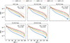 |
Fig. 6. Distributions of Δθ. The dotted lines represent the model of Eq. (4). The fitting parameters are indicated in each panel, and the distances are shown at the top of each panel. |
4. Discussion and conclusions
We presented the radial evolution of the scale-dependent magnetic field increments and rotation angle distributions in the inner heliosphere for distances to the Sun below 0.5 au. Our results show that both distributions evolve with radial distance in a scale-dependent fashion.
The increment distributions evolve towards a log-normal shape, although this evolution is different at small and large scales, here represented by the values of ⟨ΔB/B⟩ to remove the radial decay of the fluctuations due to pure expansion. At ⟨ΔB/B⟩ = 0.1, corresponding to small scales, the log-normal fit is excellent at all distances, according to the values obtained for the coefficient of determination R. For larger scales, the fit performs slightly worse, but it improves with increasing distance (Fig. 5). This highlights the scale-dependent radial evolution of the increment statistics towards a log-normal, with the small scales being approximately log-normal independent of the distance. The log-normal variance σ also shows a clear scale-dependent radial evolution, which is particularly evident for the large scales. Its value increases with distance, mostly to capture the evident evolution of the tails of the distributions.
We then used our data to validate the rotation angle model distribution proposed by Zhdankin et al. (2012) for measurements at 1 au, which assumes that the variance of the log-normal magnetic increments distribution is σ = 1. The Zhdankin et al. (2012) model fits the distributions reasonably well at small scales close to the Sun and at all scales for larger distances, with a slight discrepancy that might be due to the log-normal parameter fitting the increment PDFs being σ ≠ 1 at all the distances investigated here. However, a more evident disagreement appears at large scales near the Sun, where there are fewer large-angle rotations, which questions the universality of the model. This disagreement, and the improvement of the fit as the radial distance increases, is consistent with the evolution of σ towards unity with increasing r. As illustrated in Fig. 6, a single function based on the log-normality of the increments is thus capable of capturing most of the rotations far enough from the Sun. This result challenges the idea of the existence of two different populations of solar wind discontinuities (Borovsky 2008). Furthermore, it possibly suggests, considering the link between log-normal distributions and turbulence, that the turbulence may cause the formation of sharp rotations, as investigated in previous works (see, e.g., Zhdankin et al. 2013; Howes 2016).
The scale-dependent radial evolution of the distributions towards a log-normal is a key property to consider when investigating their origin. The observed change in shape may have two possible interpretations at least. (i) The turbulent interactions in the solar wind might reshape the distribution into a log-normal. Turbulence simulations are able to approximately produce log-normal distributions for the magnetic field vector increments, and they can reproduce the rotation distributions at 1 au (Zhdankin et al. 2012). Furthermore, log-normal distributions are observed in turbulence simulations for the scale-dependent energy dissipation rate and in solar wind data for a proxy of the same quantity (Sorriso-Valvo et al. 2015; Zhdankin et al. 2016). Turbulence interactions are faster at smaller scales. The larger scales would therefore be expected to evolve more slowly, in agreement with our results. This behaviour is also observed for the scale-dependent radial evolution of coherent structures (Sioulas et al. 2022). (ii) The change in shape could be attributed to the growth of the normalised fluctuations with the expansion, with the constraint of a constant magnetic field magnitude. This constraint has to be invoked because expansion alone can produce the growth of the amplitudes of ΔB/B (Parker 1965; Belcher 1971; Mallet et al. 2021; Squire & Mallet 2022), that is, shift the unnormalised PDFs to larger ΔB/B, resulting in a growth of large angular deflection, but it is not expected to change the shape of the PDFs (see Fig. 4). Therefore, an additional process is required to explain the full distribution of the rotations. At large scales, this constraint implies a cutoff to the distribution at ΔB/B = 2. As a consequence, the PDF changes its shape when this cutoff is reached due to the expansion-driven growth of the fluctuations. However, it is not clear why this cutoff would cause the PDFs to become log-normal, and the above interpretation would not explain why the PDFs are log-normal at small scales. Furthermore, the physical origin of the constraint is an open question as well (Barnes & Hollweg 1974; Vasquez & Hollweg 1998; Roberts 2012; Matteini et al. 2015; Tenerani & Velli 2018; Squire et al. 2019; Squire & Mallet 2022; Matteini et al. 2024).
The results presented here are also relevant to switchbacks studies. Even though using Δθ is not equivalent to using the parameter z that is typically used to identify the switchbacks (Dudok de Wit et al. 2020; Pecora et al. 2022; Jagarlamudi et al. 2023), for a given switchback duration, the increment technique still captures the full switchback structures when τ is of the order or longer than the duration of the switchback itself, and it highlights the rotation at the boundaries when it is much shorter. The radial trends of the distributions at large angles (Figs. 2 and 4) agree overall with the results in switchback studies (Tenerani et al. 2021; Pecora et al. 2022; Jagarlamudi et al. 2023; Liu et al. 2023), highlighting the presence of more large-angle deflections at greater distances.
In light of the results shown here and based on the above considerations, it seems most likely that expansion causes the overall relative amplitudes (ΔB/B) to grow, and turbulence reshapes the magnetic field rotations to create the fluctuation distributions that we measure.
Acknowledgments
We thank A. Tenerani, T. Bowen, A. Mallet, J. Squire, V. Zhdankin, L. Matteini and N. Sioulas for valuable discussions. A.L. is supported by STFC Consolidated Grant ST/T00018X/1. C.H.K.C. is supported by UKRI Future Leaders Fellowship MR/W007657/1 and STFC Consolidated Grants ST/T00018X/1 and ST/X000974/1. J.R.M. is supported by STFC studentship grant ST/V506989/1. A.L. and L.S.V. acknowledge the support of the PRIN 2022 project “2022KL38BK – The ULtimate fate of TuRbulence from space to laboratory plAsmas (ULTRA)” (Master CUP B53D23004850006) by the Italian Ministry of University and Research, funded under the National Recovery and Resilience Plan (NRRP), Mission 4 – Component C2 – Investment 1.1, “Fondo per il Programma Nazionale di Ricerca e Progetti di Rilevante Interesse Nazionale (PRIN 2022)” (PE9) by the European Union – NextGenerationEU. V.K.J. acknowledges support from the Parker Solar Probe mission as part of NASA’s Living with a Star (LWS) program under contract NNN06AA01C. L.S.V. is supported by the Swedish Research Council (VR) Research Grant 2022-03352. J.R.M. and A.L. acknowledge support from the Perren Exchange Programme. We thank the members of the FIELDS/SWEAP teams and PSP community for helpful discussions. PSP data are available at the SPDF (https://spdf.gsfc.nasa.gov).
References
- Adhikari, L., Zank, G. P., & Zhao, L. L. 2020, ApJ, 901, 102 [Google Scholar]
- Adhikari, L., Zank, G. P., Zhao, L. L., & Telloni, D. 2022, ApJ, 933, 56 [NASA ADS] [CrossRef] [Google Scholar]
- Alberti, T., Laurenza, M., Consolini, G., et al. 2020, ApJ, 902, 84 [NASA ADS] [CrossRef] [Google Scholar]
- Bale, S. D., Goetz, K., Harvey, P. R., et al. 2016, Space Sci. Rev., 204, 49 [Google Scholar]
- Bale, S. D., Badman, S. T., Bonnell, J. W., et al. 2019, Nature, 576, 237 [NASA ADS] [CrossRef] [Google Scholar]
- Bandyopadhyay, R., Matthaeus, W. H., McComas, D. J., et al. 2022, ApJ, 926, L1 [NASA ADS] [CrossRef] [Google Scholar]
- Barnes, A., & Hollweg, J. V. 1974, J. Geophys. Res., 79, 2302 [NASA ADS] [CrossRef] [Google Scholar]
- Belcher, J. W. 1971, ApJ, 168, 509 [Google Scholar]
- Borovsky, J. E. 2008, J. Geophys. Res.: Space Phys., 113, A08110 [NASA ADS] [Google Scholar]
- Borovsky, J. E. 2010, Phys. Rev. Lett., 105, 111102 [Google Scholar]
- Borovsky, J. E. 2020, Geophys. Res. Lett., 47, e84586 [NASA ADS] [CrossRef] [Google Scholar]
- Bowen, T. A., Bale, S. D., Chandran, B. D. G., et al. 2024, Nat. Astron., 8, 482 [Google Scholar]
- Bruno, R., & Carbone, V. 2013, Liv. Rev. Sol. Phys., 10, 2 [Google Scholar]
- Bruno, R., Carbone, V., Primavera, L., et al. 2004, Ann. Geophys., 22, 3751 [Google Scholar]
- Burlaga, L. F. 2001, J. Geophys. Res., 106, 15917 [NASA ADS] [CrossRef] [Google Scholar]
- Castaing, B., Gagne, Y., & Hopfinger, E. J. 1990, Phys. D Nonlinear Phenom., 46, 177 [NASA ADS] [CrossRef] [Google Scholar]
- Chandran, B. D. G., & Perez, J. C. 2019, J. Plasma Phys., 85, 905850409 [NASA ADS] [CrossRef] [Google Scholar]
- Chen, C. H. K., Matteini, L., Burgess, D., & Horbury, T. S. 2015, MNRAS, 453, L64 [NASA ADS] [CrossRef] [Google Scholar]
- Chen, C. H. K., Bale, S. D., Bonnell, J. W., et al. 2020, ApJS, 246, 53 [Google Scholar]
- Cuesta, M. E., Chhiber, R., Fu, X., et al. 2023, ApJ, 949, L19 [NASA ADS] [CrossRef] [Google Scholar]
- D’Amicis, R., Perrone, D., Bruno, R., & Velli, M. 2021, J. Geophys. Res.: Space Phys., 126, e28996 [Google Scholar]
- Davis, N., Chandran, B. D. G., Bowen, T. A., et al. 2023, ApJ, 950, 154 [NASA ADS] [CrossRef] [Google Scholar]
- Dong, Y., Verdini, A., & Grappin, R. 2014, ApJ, 793, 118 [Google Scholar]
- Dudok de Wit, T., Krasnoselskikh, V. V., Bale, S. D., et al. 2020, ApJS, 246, 39 [Google Scholar]
- Frisch, U. 1995, Turbulence: The Legacy of A. N. Kolmogorov (Cambridge: Cambridge University Press) [Google Scholar]
- Greco, A., & Perri, S. 2014, ApJ, 784, 163 [NASA ADS] [CrossRef] [Google Scholar]
- Greco, A., Chuychai, P., Matthaeus, W. H., Servidio, S., & Dmitruk, P. 2008, Geophys. Res. Lett., 35, L19111 [Google Scholar]
- Hernández, C. S., Sorriso-Valvo, L., Bandyopadhyay, R., et al. 2021, ApJ, 922, L11 [CrossRef] [Google Scholar]
- Howes, G. G. 2016, ApJ, 827, L28 [NASA ADS] [CrossRef] [Google Scholar]
- Huang, S. Y., Sahraoui, F., Andrés, N., et al. 2021, ApJ, 909, L7 [NASA ADS] [CrossRef] [Google Scholar]
- Huang, J., Kasper, J. C., Fisk, L. A., et al. 2023a, ApJ, 952, 33 [NASA ADS] [CrossRef] [Google Scholar]
- Huang, Z., Sioulas, N., Shi, C., et al. 2023b, ApJ, 950, L8 [NASA ADS] [CrossRef] [Google Scholar]
- Jagarlamudi, V. K., Raouafi, N. E., Bourouaine, S., et al. 2023, ApJ, 950, L7 [NASA ADS] [CrossRef] [Google Scholar]
- Kasper, J. C., Abiad, R., Austin, G., et al. 2016, Space Sci. Rev., 204, 131 [Google Scholar]
- Kasper, J. C., Bale, S. D., Belcher, J. W., et al. 2019, Nature, 576, 228 [Google Scholar]
- Krasnoselskikh, V., Larosa, A., Agapitov, O., et al. 2020, ApJ, 893, 93 [Google Scholar]
- Larosa, A., Krasnoselskikh, V., Dudok de Wit, T., et al. 2021, A&A, 650, A3 [EDP Sciences] [Google Scholar]
- Li, G. 2008, ApJ, 672, L65 [NASA ADS] [CrossRef] [Google Scholar]
- Liu, Y. D., Ran, H., Hu, H., & Bale, S. D. 2023, ApJ, 944, 116 [NASA ADS] [CrossRef] [Google Scholar]
- Mallet, A., Squire, J., Chandran, B. D. G., Bowen, T., & Bale, S. D. 2021, ApJ, 918, 62 [NASA ADS] [CrossRef] [Google Scholar]
- Matteini, L., Horbury, T. S., Pantellini, F., Velli, M., & Schwartz, S. J. 2015, ApJ, 802, 11 [Google Scholar]
- Matteini, L., Stansby, D., Horbury, T. S., & Chen, C. H. K. 2018, ApJ, 869, L32 [Google Scholar]
- Matteini, L., Tenerani, A., Landi, S., et al. 2024, Phys. Plasmas, 31, 032901 [NASA ADS] [CrossRef] [Google Scholar]
- McIntyre, J. R., Chen, C. H. K., & Larosa, A. 2023, ApJ, 957, 111 [NASA ADS] [CrossRef] [Google Scholar]
- Meyrand, R., Squire, J., Schekochihin, A. A., & Dorland, W. 2021, J. Plasma Phys., 87, 535870301 [CrossRef] [Google Scholar]
- Owens, M. J., Wicks, R. T., & Horbury, T. S. 2011, Sol. Phys., 269, 411 [NASA ADS] [CrossRef] [Google Scholar]
- Palacios Caicedo, J. C. 2021, Doctoral Dissertation, Florida Institute of Technology [Google Scholar]
- Parker, E. N. 1965, Space Sci. Rev., 4, 666 [Google Scholar]
- Pecora, F., Matthaeus, W. H., Primavera, L., et al. 2022, ApJ, 929, L10 [NASA ADS] [CrossRef] [Google Scholar]
- Perez, J. C., & Chandran, B. D. G. 2013, ApJ, 776, 124 [Google Scholar]
- Perri, S., Yordanova, E., Carbone, V., et al. 2009, J. Geophys. Res.: Space Phys., 114, A02102 [NASA ADS] [CrossRef] [Google Scholar]
- Perrone, D., D’Amicis, R., De Marco, R., et al. 2020, A&A, 633, A166 [EDP Sciences] [Google Scholar]
- Pezzi, O., Parashar, T. N., Servidio, S., et al. 2017, J. Plasma Phys., 83, 705830108 [NASA ADS] [CrossRef] [Google Scholar]
- Raouafi, N. E., Matteini, L., Squire, J., et al. 2023, Space Sci. Rev., 219, 8 [NASA ADS] [CrossRef] [Google Scholar]
- Roberts, D. A. 2012, Phys. Rev. Lett., 109, 231102 [NASA ADS] [CrossRef] [Google Scholar]
- Ruffolo, D., Matthaeus, W. H., Chhiber, R., et al. 2020, ApJ, 902, 94 [Google Scholar]
- Shi, C., Velli, M., Panasenco, O., et al. 2021, A&A, 650, A21 [NASA ADS] [CrossRef] [Google Scholar]
- Shi, C., Sioulas, N., Huang, Z., et al. 2023, ArXiv e-prints [arXiv:2308.12376] [Google Scholar]
- Sioulas, N., Huang, Z., Velli, M., et al. 2022, ApJ, 934, 143 [CrossRef] [Google Scholar]
- Sioulas, N., Velli, M., Huang, Z., et al. 2023a, ApJ, 951, 141 [CrossRef] [Google Scholar]
- Sioulas, N., Huang, Z., Shi, C., et al. 2023b, ApJ, 943, L8 [CrossRef] [Google Scholar]
- Sorriso-Valvo, L., Carbone, V., Veltri, P., Consolini, G., & Bruno, R. 1999, Geophys. Res. Lett., 26, 1801 [NASA ADS] [CrossRef] [Google Scholar]
- Sorriso-Valvo, L., Marino, R., Lijoi, L., Perri, S., & Carbone, V. 2015, ApJ, 807, 86 [NASA ADS] [CrossRef] [Google Scholar]
- Sorriso-Valvo, L., Marino, R., Foldes, R., et al. 2023, A&A, 672, A13 [NASA ADS] [CrossRef] [EDP Sciences] [Google Scholar]
- Squire, J., & Mallet, A. 2022, ArXiv e-prints [arXiv:2206.07447] [Google Scholar]
- Squire, J., Schekochihin, A. A., Quataert, E., & Kunz, M. W. 2019, J. Plasma Phys., 85, 905850114 [NASA ADS] [CrossRef] [Google Scholar]
- Squire, J., Chandran, B. D. G., & Meyrand, R. 2020, ApJ, 891, L2 [Google Scholar]
- Telloni, D., Sorriso-Valvo, L., Woodham, L. D., et al. 2021, ApJ, 912, L21 [NASA ADS] [CrossRef] [Google Scholar]
- Tenerani, A., & Velli, M. 2018, ApJ, 867, L26 [Google Scholar]
- Tenerani, A., Sioulas, N., Matteini, L., et al. 2021, ApJ, 919, L31 [NASA ADS] [CrossRef] [Google Scholar]
- Trotta, D., Pezzi, O., Burgess, D., et al. 2023, MNRAS, 525, 1856 [NASA ADS] [CrossRef] [Google Scholar]
- Vasquez, B. J., & Hollweg, J. V. 1998, J. Geophys. Res., 103, 349 [NASA ADS] [CrossRef] [Google Scholar]
- Verdini, A., & Grappin, R. 2015, ApJ, 808, L34 [NASA ADS] [CrossRef] [Google Scholar]
- Whittlesey, P. L., Larson, D. E., Kasper, J. C., et al. 2020, ApJS, 246, 74 [Google Scholar]
- Zank, G. P., Nakanotani, M., Zhao, L. L., Adhikari, L., & Kasper, J. 2020, ApJ, 903, 1 [NASA ADS] [CrossRef] [Google Scholar]
- Zhao, L.-L., Zank, G. P., Telloni, D., et al. 2022, ApJ, 928, L15 [NASA ADS] [CrossRef] [Google Scholar]
- Zhdankin, V., Boldyrev, S., & Mason, J. 2012, ApJ, 760, L22 [NASA ADS] [CrossRef] [Google Scholar]
- Zhdankin, V., Uzdensky, D. A., Perez, J. C., & Boldyrev, S. 2013, ApJ, 771, 124 [NASA ADS] [CrossRef] [Google Scholar]
- Zhdankin, V., Boldyrev, S., & Chen, C. H. K. 2016, MNRAS, 457, L69 [NASA ADS] [CrossRef] [Google Scholar]
- Zhu, X., He, J., Verscharen, D., Duan, D., & Bale, S. D. 2020, ApJ, 901, L3 [NASA ADS] [CrossRef] [Google Scholar]
All Tables
Values in seconds of the lag we used for different distances and different average values of ⟨ΔB/B⟩ to compute the increments.
All Figures
|
Fig. 1. Distributions of the magnetic field increments ΔB/B. The increments are computed at different timescales, τ, for each panel, as indicated at the top. The different colours represent different heliocentric distances. The shaded area represents the statistical error estimated as the square root of the number of points in a given bin. The error is not visible in most cases because it is small and comparable with the width of the plot lines. |
| In the text | |
|
Fig. 2. Distributions of the magnetic deflection angles Δθ. The order of the panels and the meaning of the colours is the same as in Fig. 1. |
| In the text | |
|
Fig. 3. Distributions of χ, the normalised difference between the magnetic vector increments and the corresponding angle if this were due to pure rotation. The different colors represent different values of τ. The solid lines are drawn at distances below 0.1 au, and the dotted lines are drawn at distances between 0.4 and 0.5 au. |
| In the text | |
|
Fig. 4. Distributions of the magnetic deflection angles Δθ at fixed values of the average increment value ⟨ΔB/B⟩. |
| In the text | |
|
Fig. 5. Distributions of the magnetic field vector increments at fixed average ΔB/B. The dashed lines are log-normal fits to the data. The bottom right panel shows the variation with distance and scale of the parameter σ. |
| In the text | |
|
Fig. 6. Distributions of Δθ. The dotted lines represent the model of Eq. (4). The fitting parameters are indicated in each panel, and the distances are shown at the top of each panel. |
| In the text | |
Current usage metrics show cumulative count of Article Views (full-text article views including HTML views, PDF and ePub downloads, according to the available data) and Abstracts Views on Vision4Press platform.
Data correspond to usage on the plateform after 2015. The current usage metrics is available 48-96 hours after online publication and is updated daily on week days.
Initial download of the metrics may take a while.