| Issue |
A&A
Volume 697, May 2025
|
|
|---|---|---|
| Article Number | A187 | |
| Number of page(s) | 9 | |
| Section | The Sun and the Heliosphere | |
| DOI | https://doi.org/10.1051/0004-6361/202553848 | |
| Published online | 19 May 2025 | |
A new scenario with two subranges in the inertial regime of solar wind turbulence
1
School of Earth and Space Science and Technology, Wuhan University, Wuhan, PR China
2
School of Earth and Space Sciences, Peking University, Beijing, PR China
3
SIGMA Weather Group, State Key Laboratory for Space Weather, National Space Science Center, Chinese Academy of Sciences, Beijing, PR China
4
Space and Plasma Physics, School of Electrical Engineering and Computer Science, KTH Royal Institute of Technology, Stockholm, Sweden
5
Institute for the Science and Technology of Plasmas, National Research Council, Bari, Italy
6
School of Space and Earth Sciences, Beihang University, Beijing, PR China
⋆ Corresponding author: This email address is being protected from spambots. You need JavaScript enabled to view it.
Received:
22
January
2025
Accepted:
26
March
2025
Abstract
Context. The solar wind provides a natural laboratory for plasma turbulence. The core problem is the energy cascade process in the inertial range, which has been a fundamental long-standing question. Much effort has been put into theoretical models to explain the observational features in the solar wind. However, there are still many questions that remain unanswered.
Aims. Here, we report the observational evidence for the existence of two subranges in the inertial regime of the solar wind turbulence and show the scaling features for each subranges.
Methods. We performed multi-order structure function analyses for one high-latitude fast solar wind interval at 1.48 au measured by Ulysses and one slow but Alfvénic solar wind at 0.17 au measured by the Parker Solar Probe (PSP). We also conducted statistical analyses on 103 fast solar wind intervals observed by Wind.
Results. We identify the existence of two subranges in the inertial range according to the distinct scaling features of the magnetic field. The multi-order scaling indices versus the order for the two subranges demonstrates a clear disparity, with the second-order scaling index being 1/2 in the larger-scale subrange 1 and 2/3 in the smaller-scale subrange 2. Both subranges display apparent but different anisotropies. The velocity exhibits similar features as the magnetic field. The PSP interval shows that subrange 1 follows Yaglom scaling law, while subrange 2 does not. The Ulysses interval shows that the intermittency abruptly grows to a maximum 5% of the interval from subrange 1 to subrange 2.
Conclusions. Based on the observational features, we propose a new scenario that the inertial regime of the solar wind turbulence consists of two subranges. The observational evolution of the scaling as the solar wind expands may be a consequence of observing different subranges at different radial distances.
Key words: Sun: heliosphere / Sun: magnetic fields / solar wind
© The Authors 2025
 Open Access article, published by EDP Sciences, under the terms of the Creative Commons Attribution License (https://creativecommons.org/licenses/by/4.0), which permits unrestricted use, distribution, and reproduction in any medium, provided the original work is properly cited.
This article is published in open access under the Subscribe to Open model. This email address is being protected from spambots. You need JavaScript enabled to view it. to support open access publication.
1. Introduction
Plasma turbulence is a fundamental physical process that transfers the energy between different spatial scales (Verscharen et al. 2019). It permeates the Universe (Schekochihin & Cowley 2007) and plays an important role in cutting-edge questions such as the cosmic magnetic fields dynamo (Schekochihin et al. 2004) and the solar corona and solar wind heating (Bruno & Carbone 2013). It remains an unsolved and intriguing problem after decades of endeavor to develop the theories. Since the power-law behavior of the magnetic field spectrum was identified (Coleman 1968), the solar wind has been an excellent natural laboratory for the investigation of plasma turbulence.
The basic approach to analyze the nonlinear dynamics underlying solar wind turbulence is to observe the spectral index in the inertial range, whose value is the primary task for the theory to explain. The Kolmogorov theory (Kolmogorov 1941, hereafter K41) assumes that the nonlinear interaction occurs between isotropic velocity eddies with similar spatial scales and predicts an index of −5/3 for the velocity spectrum. Iroshnikov (Iroshnikov 1964) and Kraichnan (Kraichnan 1965) adapted the K41-type thinking to magnetic fluids but proposed that the nonlinear interaction in plasmas happens between the Alfvén wavepackets travelling in opposite directions instead. The resulting index becomes −3/2 for both magnetic field and velocity spectra. However, the 1D power spectra in the solar wind at 1 au display variable scaling exponents, with a prevalence of −3/2 for velocity and −5/3 for the magnetic field (Podesta et al. 2007; Salem et al. 2009).
The inconsistent solar wind observations with these two simplest but still not fully understood isotropic turbulence models highlight the requirements to advance the physical understanding of turbulent magnetic fluid. One of the crucial developments is to abandon the isotropy assumption due to the magnetic field. Theoretical interpretation of the anisotropy of solar wind turbulence can be divided into two main classes. One is the so-called 2D-slab and the other is the critical balance. Matthaeus et al. (1990) found that the 2D self-correlation function level contours consist of two lobes, displaying the famous “Maltese cross” pattern. This result pioneered the concept that solar wind turbulence is composed of slab-like fluctuations (the lobe elongated along the perpendicular direction to the mean field direction) and 2D fluctuations (the lobe elongated along to the mean field direction). The critical balance model (Goldreich & Sridhar 1995) conjectures that strong turbulence tends toward a state of critical balance, in which the timescale of the Alfvénic fluctuations propagating along the magnetic field is equal to the timescale of their nonlinear decay. This model successfully explains the magnetic spectral index transition from −2 to −5/3 when measuring from parallel to perpendicular to the local magnetic field in the solar wind (Horbury et al. 2008). We note, however, that the use of a local, scale-dependent mean field to condition the statistics comes with some criticisms (e.g., see Oughton & Matthaeus 2020; Telloni et al. 2019). Further refinements consider the dynamic-alignment effect (Boldyrev 2006), the imbalanced version (Lithwick et al. 2007), and the solar wind expansion (Verdini & Grappin 2015). Despite over 60 years of research and many major advances, a satisfactory theory of magnetohydrodynamic (MHD) turbulence remains elusive. The difference between the magnetic field and velocity is one of the principal puzzles.
New observations obtained by PSP reveal that the spectral index evolves from −3/2 to −5/3 in the inertial range from the near-Sun region to 1 au (Chen et al. 2020) and the spectral index is close to −5/3 in the parallel direction and near −2/3 in the perpendicular direction (Huang et al. 2022), imposing new puzzles to be solved by the theoretical model. The gap of the spectral index between −3/2 and −5/3 is too small to be distinguished considering the uncertainty (Smith et al. 2006a; Podesta 2009) or to be identified on the spectrum by eye (Wicks et al. 2011; Telloni 2022). When Telloni (2022) fit the power spectrum for two subranges in a stream originating from the same source observed by PSP, they obtained −3/2 and −5/3, respectively. The existence of two subranges remains to be questioned.
The multi-order structure function approach can reveal the features of scaling laws hidden to the usual spectral (second order) methods (Sorriso-Valvo et al. 2023) and provide more information. In this study, we perform multi-order structure function analyses and identify two subranges in the inertial regime of solar wind turbulence for two streams observed by Ulysses and PSP and confirm the existence of the two subranges with statistical results of 103 fast solar wind intervals observed by Wind. We propose a new scenario: that the solar wind turbulence contains two distinct regimes in the inertial range. This scenario is rooted in the observational features and provides a possible explanation for the above-mentioned puzzles. This paper is organized as follows. In Sect. 2, we describe the measurements and the method to reveal the existence of two subranges. In Sect. 3, we present the results. In Sect. 4, we discuss our results and draw our conclusions.
2. Data and method
We performed multi-order structure function analyses for two intervals. The first interval was measured by Ulysses at r∼1.48 au and a latitude of ϕ∼47° from May 1 to May 10, 1995, with an average flow speed of V0 = 771 km/s and proton beta of β = 1.20. The magnetic field data was obtained by the Vector Helium Magnetometer (Balogh et al. 1992) with a time resolution of 1 s. The data gap is less than 2% and we made an interpolation at times with a uniform time cadence of 1 s. During this period, Ulysses passed the polar region and pertained to high-speed flows with speeds greater than 700 km/s. This polar pass of Ulysses provides the measurement of the same stream originating from the polar corona for a long time outside 1 au. The second interval is a near-Sun solar wind interval obtained by PSP (Fox et al. 2016) during its first encounter within November 6 to November 7, 2018, when r∼0.17 au, V0 = 332 km/s, and β = 0.54. Both the magnetic field data from the fluxgate magnetometer in the FIELDS instrument suite (Bale et al. 2016) and the plasma data from the Solar Probe Cup (Case et al. 2020) of Solar Wind Electrons, Protons, and Alphas instrument suite (Kasper et al. 2016) have a time resolution of 0.8738 s. The data gap is less than 1% for the magnetic field and 8% for plasma. We made an interpolation with a uniform time cadence of 0.8738 s. This interval has been shown to originate from a small negative equatorial coronal hole (Badman et al. 2020). The cross helicity, whose value weighs the Alfvénicity, is −0.75 for the Ulysses interval and 0.84 for the PSP interval. Both intervals show high Alfvénicity and neither of them contains strong shear flows or interaction regions, as is shown by the time series in Fig. 1. They were chosen since they are representative of a typical solar wind with a robust stationarity and homogeneity, and have been characterized in depth in the past (Wicks et al. 2010; Forman et al. 2011; Chen et al. 2012; Pei et al. 2016; Chhiber et al. 2021; Wu et al. 2023a).
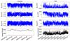 |
Fig. 1. Time series of three components of magnetic field (blue) in RTN coordinates and the flow speed (black) for the Ulysses interval (left) and the PSP interval (right). The dashed red lines denote the speed of 500 km/s. The time is indicated as year-month-day, in UTC for the Ulysses interval and as hour-minutes-seconds, in UTC for the PSP interval. |
We also conducted multi-order structure function analyses of the magnetic field data from the magnetic field investigation (Lepping et al. 1995) and the plasma data from the 3D plasma analyzer (Lin et al. 1995) on board Wind. Both datasets have a time resolution of 3 s. We selected all the ≥2 days fast solar wind intervals with solar wind speeds larger than 500 km/s from 2005 to 2018 when Wind hovers at the Lagrangian point L1. We restricted the proton number density to [1, 5] cm−3 to remove the effect of interplanetary corona mass ejections. Eventually, we obtained 103 fast solar wind intervals without strong shear flows or interaction regions.
The multi-order structure function is calculated by the moments of the increments δU(t, τ) of the variables (U is either the magnetic field, B, or velocity, V, in this study). The increment, δU, is the difference between two instants, varying with both time and scale. It can be calculated as
 (1)
(1)
where τ is the time lag. The q-th order structure functions are defined as
 (2)
(2)
where 〈〉 denotes an ensamble time average. We calculated the local background magnetic field, B0(t, τ), as an average in the moving scale-dependent window (Chen et al. 2012). The sampling angle, θ(t, τ), was obtained between the local magnetic field direction and the radial direction for the Ulysses interval and between the local background magnetic field and the flow velocity for the PSP and Wind intervals. The increments, δU(t, τ), were selected under the criteria of a different sampling angle (80°<θ(t, τ)<100° and θ(t, τ)<10° or θ(t, τ)>170°) to obtain Sq(τ⊥) and Sq(τ∥). For single spacecraft observations, the spatial lag is L=τV0 under the Taylor hypothesis (Taylor 1938). It is further normalized by the ion inertial length, di=c/ωpi (where  , mp is the proton mass, and np is the number density of the solar wind) to reveal the underlying processes on a physically constant scale.
The higher-order structure functions play a crucial role in the turbulence theory and the scaling properties can reflect the cascade process (Biskamp 2003). Sq(l) exhibits the scaling behavior as
 (3)
(3)
Eq. (3) contains full information on the specific range and the negative of the scaling indices ξ(2) can be converted to the spectral index, α, as α=−ξ(2)−1 (Monin & Yaglom 1975). Here, we perform power law fits at two different ranges in the inertial region and obtain multi-order scaling indices in different sampling directions, including ξ(q), ξ⊥(q), ξ∥(q) from Sq(τ), Sq(τ⊥), and Sq(τ∥) for these two subranges, respectively. We estimated the maximum reliable order, qmax, following the procedure in Dudok de Wit (2004). The absolute values of the magnetic field increments, δB(t, τ), were sorted in decreasing order to be δB(k, τ) with the indices, k, representing the position. The peak of δB(k, τ) with respect to k is well described by a power law, δB(k, τ) = αk−γ(τ). We performed the power-law fits for different sets of δB(k, τ) and obtained γ(τ). The maximum moment, qmax, that can be meaningfully estimated was determined as ![Mathematical equation: $ q_{\mathrm {max}} = [\frac {1}{\gamma }]-1 $](/articles/aa/full_html/2025/05/aa53848-25/aa53848-25-eq5.gif) , in which [] denotes the integer part. We obtained the wavevector anisotropy, k⊥ versus k∥, by calculating the spatial lag (L = 2π/k) for each second-order structure function level,
, in which [] denotes the integer part. We obtained the wavevector anisotropy, k⊥ versus k∥, by calculating the spatial lag (L = 2π/k) for each second-order structure function level,  , with
  (Chen et al. 2012).
The partial variance of increments (PVI) method is to classify the intermittent structures by setting a threshold on the PVI values (Greco et al. 2018). The PVI is defined in terms of the magnetic field increment as
 (4)
(4)
We adopted a recursive method to determine the required threshold, Ithres (Veltri 1999; Wu et al. 2023b), until the flatness, F, of the increments with PVI>Ithres is close enough to 3, a value for a Gaussian distribution. The flatness, F, is another parameter to evaluate the intermittency and is defined as
 (5)
(5)
The percentage is obtained as the ratio between the numbers of the increments with PVI>PVIgauss and all increments.
The Yaglom scaling law is an exact relation derived for the mixed third-order structure functions directly from the dynamical MHD equations with the assumption of homogeneity and isotropy (Politano & Pouquet 1998). The mixed third-order structure functions are defined as
 (6)
(6)
where ΔZ±(x, l) = Z±(x+l)−Z±(x) is the increment of the Elsässer variables, Z±, at position x and spatial scale l. Elsässer variables are defined as Z±(x) = V(x)±VA(x), in which  is the magnetic field in Alfvén units. The Yaglom scaling law can be expressed as
  , where ϵ± is the energy cascade rate for the respective Elsässer energies per unit mass in the inertial range. The total cascade rate, ϵ, is the average of ϵ+ and ϵ−. The mixed third-order structure functions were obtained as a function of the temporal lags, τ, for single-spacecraft observations with L=τV0, and the total third-order structure function, Y=(Y++Y−)/2, can be written as
 (7)
(7)
With the Yaglom scaling law satisfied, the energy cascade rate can be estimated by the slope obtained from the linear fitting of Y(τ).
The von Kármán decay describes the decay of energy-containing eddies in hydrodynamics (von Karman & Howarth 1938). The von Kármán decay rate measures the energy flux fed into the inertial range to be transferred to smaller scales. It is generalized to MHD (Hossain et al. 1995; Wan et al. 2012) as:
 (8)
(8)
Here, α± are constants and α+∼α− = 0.03 in MHD turbulence (Linkmann et al. 2015). δZ± are the amplitudes of Elsässer variables fluctuations and are calculated by δZ±=〈z±2〉1/2, where  and
and  is the average of Z±.
The self-correlation function describes the similarity between the variable and a delayed copy of itself as a function of the delayed time lag. Therefore, in order to obtain the similarity length scales, L±, we calculated the two-time-point self-correlation function, z± as R±(τ) = 〈z±(t)·z±(t+τ)〉. The normalized self-correlation function is NCF±(τ) = R±(τ)/R±(0), so that NCF±(0) is always equal to 1. It is convenient to obtain the correlation scale using the 1/e definition (Smith et al. 2001): NCF±(τ±) = 1/e, where e is the base of the natural logarithm. Thus, we obtained L±=τ±V0. The total von Kármán decay rate is  .
.
3. Results
Sq(τ) detected in the radial direction, and Sq(τ⊥) and Sq(τ∥) detected in the directions perpendicular and parallel to the local magnetic field for the 10-day Ulysses interval, respectively, are shown in Figs. 2a–c. Sq(τ∥) displays the most distinctive subranges, 10<τ<100 s and 100<τ<1000 s, within the normally considered inertial range determined by the power spectra (Bruno & Carbone 2013). The transition is located at 100 seconds and becomes clearer as the order goes higher. We refer to 100<τ<1000 s as subrange 1 and 10<τ<100 s as subrange 2 for this interval.
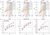 |
Fig. 2. Structure functions and scaling indices of magnetic field in the fast solar wind at 1.48 au observed by Ulysses. (a)–(c) Sq versus τ (bottom axis) and L (upper axis, in unit of the ion inertial length, di) measured in the radial direction, and in the directions perpendicular and parallel to the local magnetic field, respectively. The blue, orange, green, red, and purple represent Sq of order q = 1, 2, 3, 4, 5, respectively. The dashed yellow and cyan lines are power-law fits to Sq in subranges 1 and 2, shown with red and black shadows, respectively. (d)–(f) ξ(q), ξ⊥(q), ξ∥(q). The black and red represent the results in subrange 1 and 2, respectively. The horizontal dashed lines denote ξ = 1/2, 2/3, 1, respectively. The standard errors of these indices are small and no larger than the size of the markers. |
The scaling indices versus order q for both subrange 1 and 2 are illustrated by Figs. 2d–f, in which the indices with higher than the maximum order qmax are marked in hollow style. The standard errors of these indices are close to the standard errors that fit within a single inertial range and are all smaller than 0.011 in the radial direction, 0.012 in the perpendicular direction, 0.053 in the parallel direction. We find distinct features between two subranges. For higher orders, the differences between the two subranges are more obvious. Figure 2d shows that both subrange 1 and 2 have multifractal scaling, visible as deviation from linear dependence of ξ(q) on the order q. For subrange 1, ξ(2)∼1/2, while for subrange 2, ξ(2)∼2/3. This agrees with the omnidirectional spectral indices for the near-Sun solar wind from the same flow tube measured by PSP (Telloni 2022). Figure 2e shows that both subranges are multifractal measured in the perpendicular direction and ξ⊥(2) is closer to 1/2 in subrange 1 and 2/3 in subrange 2. Figure 2f displays the scaling detected in the parallel direction. Subrange 1 is multifractal with ξ∥(2)∼2/3, while subrange 2 is nearly monoscaling with ξ∥(2) closer to 1. The scaling for the subrange 2 is consistent with the observations at 1 au obtained by Stereo spacecraft (Osman et al. 2014).
Figure 3a presents Sq(τ) of the magnetic field for the PSP interval. The red and black shadows share the same spatial scales in units of di as the shadows in Fig. 2a, of which the scaling indices have shown the existence of the two subranges. ξ(q) shown in Fig. 3b is obtained within the red and black shadow ranges separately. We find that both the magnetic field and velocity clearly illustrate the existence of two subranges and they share very similar scaling for each subrange.
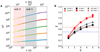 |
Fig. 3. Structure functions and the scaling indices in the slow solar wind at 0.17 au observed by PSP. (a) Sq for the magnetic field measured in the radial direction with the same formats as Fig. 2. (b) ξ(q) for both the magnetic field (triangles) and velocity (squares) obtained from PSP and for the magnetic field (circles) obtained from Ulysses. The black and red represent the results in subrange 1 and 2, respectively. The horizontal dashed lines denote ξ = 1/2 and ξ = 2/3. |
Figure 3b also demonstrates that ξ from Ulysses and PSP observations overlap surprisingly in subrange 2 from the first to the fifth order and are adjacent in subrange 1. This indicates that the two distinct subranges share the same scaling properties for both intervals and have already formed in the near-Sun solar wind turbulence. It is not easy to differentiate those two subranges from only Sq(τ) by eye and it seems to be unnecessary to use two power law fits, which may explain why the differences between the two subranges are easily overlooked in previous works and the inertial range is believed to be single power law for decades. However, when we apply the multi-order structure function approach, the higher-order statistics distinguishes the two subranges evidently. The second-order spectrum analysis may not uncover the existence of the two subranges due to the measurement uncertainty. We also investigated the anisotropy for the PSP interval. The scalings in subrange 1 observed in the parallel and perpendicular direction by PSP both almost overlap with the ones of Ulysses (now shown), while in subrange 2, the trustworthy highest order is too low for us to be able to draw a conclusion.
The timescales of subrange 2 and 1 for PSP interval at 0.17 au are around 1.5<τ<15 s and 15<τ<150 s, approximately an order lower than the ones for the interval at 1.48 au observed by Ulysses. Since the two intervals both originate from coronal holes and with high Alfvénicity, the comparison between the two intervals suggests the possibility that the differences between the near-Sun and near-Earth solar wind could result from the existence of two subranges in the inertial range and the evolution of ion inertial length, di, which makes the frequency range to be analyzed move from a physically larger range to a physically smaller range; that is, from subrange 1 (360di−3600di) to subrange 2 (36di−360di). However, while the analysis of these two intervals illustrates a case study for the Alfvénic solar wind, other factors, such as a latitudinal dependence or solar wind variability, cannot be excluded. Hence, whether the observed properties have general validity needs to be further investigated.
To substantiate with statistics the observations described above for two case studies, Fig. 4 shows the averaged scaling indices of magnetic field for 103 Wind intervals in both subrange 1 (360di−3600di) and subrange 2 (36di−360di). They are very close to the corresponding values obtained from the Ulysses intervals, sharing the same features of two subranges and anisotropy. This confirms the existence of the two subranges from a statistical perspective.
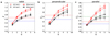 |
Fig. 4. Averaged scaling indices of magnetic field versus the order measured by Wind in the radial direction (a), and in the directions perpendicular (b) and parallel (c) to the local magnetic field. The stars (dots) denote the results from Wind (Ulysses). The black and red represent the results in subrange 1 and 2. The horizontal dashed lines denote ξ = 1/2, 2/3, 1, respectively. The standard errors of these indices are shown by error bars. |
Figure 5 displays the count distributions of the second-order scaling indices for both magnetic field and velocity of the 103 Wind intervals in both subrange 1 (360di−3600di) and subrange 2 (36di−360di). The distributions of two subranges are well separated from each other for both magnetic field and velocity in the radial and perpendicular directions. The averaged values for the magnetic field are 0.54 (0.51) in subrange 1 and 0.70 (0.67) in subrange 2 in the radial (perpendicular) direction, close to 1/2 and 2/3, respectively, while they are 0.47 (0.44) and 0.60 (0.56) for the velocity. In the parallel direction, the distributions of two subranges are different but not as well separated as the other two directions.
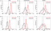 |
Fig. 5. Top: Count distribution of the second-order scaling indices for magnetic field measured by Wind in the radial direction (a), and in the directions perpendicular (b) and parallel (c) to the local magnetic field. Black and red denote subranges 1 and 2. The top right corners show the averages with their standard deviations. Bottom: Distribution of the second-order scaling indices of velocity in the same format as the top panels. |
To obtain a more detailed insight into the properties of turbulence, we performed case studies of the second-order structure functions analysis for the Ulysses interval and the mixed third-order structure functions analysis for the PSP interval. Figure 6a presents second-order structure functions of the Ulysses interval. It exhibits two distinct subranges, 10<τ<100 s and 100<τ<1000 s. Subrange 1 shows ξ∥(2) = 0.68 and ξ⊥(2) = 0.50, while subrange 2 shows ξ∥(2) = 0.90 and ξ⊥(2) = 0.62. The spectral index anisotropy in subrange 1 is similar to that in previous works found using the spectral method (Wicks et al. 2011) for a fast solar wind interval observed by Wind spacecraft. However, it is the first time that anybody has distinguished the spectral index anisotropy in subrange 1 with ξ∥(2) close to 2/3 and ξ⊥(2) close to 1/2. This also rationalizes the fact that the magnetic spectral index determined within a subrange of the inertial range is often not distinguishable between −3/2 and −5/3 (Podesta 2009; Smith et al. 2006b), which hinders a consensus on the theoretical construction. The inset panel of Fig. 6a displays k∥ versus k⊥. It shows obvious wavevector anisotropy with  throughout the entire inertial range, without a break between the two subranges. At the outer scale, k∥ and k⊥ are nearly the same.
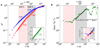 |
Fig. 6. (a) Second-order structure functions of magnetic field for the Ulysses interval. Black and red shadows denote subranges 1 and 2. Blue and red dots represent S2(τ⊥) and S2(τ∥). The numbers with the colors show the power law fit indices for the corresponding dots and the dashed lines with these indices are plotted to guide the eye. Inset: k∥ versus k⊥ for the same S2 level. (b) Mixed third-order structure functions Y for the PSP interval. The linear fit in subrange 1 is shown by dashed lines, which are used to evaluate the cascade rates. Inset: Y+ (blue) and Y− (red). |
The mixed third-order structure function (Marino & Sorriso-Valvo 2023) for the PSP interval shown in Fig. 6b further distinguishes the two distinct subranges. The Yaglom scaling law is satisfied in subrange 1 but not in subrange 2. Our results show that the second-order scaling index is close to 1/2 in the subrange 1 with Yaglom scaling and 2/3 in the subrange 2 without Yaglom scaling. This is consistent with the finding for the magnetic spectrum in Marino et al. (2012) that regions with Yaglom scaling have a shallower inertial range compared to ones without Yaglom scaling. The satisfaction of the Yaglom scaling law in subrange 1 estimates the cascade rate to be 5.27×10⁻¹⁴ W/m3. This value is very close to the von Kármán decay rate of 5.56×10⁻¹⁴ W/m3. Separate Y+ and Y− shown in the inset panel of Fig. 6b do not have a linear relationship with respect to scale. We conjecture that the nonlinear interaction in subrange 1 is driven by the decay of energy-containing eddies and is completed with both Elsässer variables playing important roles.
Finally, we utilized the PVI method to identify the intermittent instants where most of the energy is accumulated for the Ulysses interval. Figure 7 presents how the percentage of the volume occupied by intermittent structures grows rapidly from less than 0.1% to over 1% nearby the break between subrange 1 and 2 as the scale decreases. The intermittency in the parallel direction reaches the maximum earlier than the one in the perpendicular direction and they both reach a maximum around 5% in subrange 2. The percentage of intermittency for the PSP interval has been reported by Wu et al. (2023b), which showed similar properties.
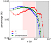 |
Fig. 7. Percentage of the intermittency for the Ulysses interval. Green, blue, and red represent the measurements in the radial direction, and in the directions perpendicular and parallel to the local magnetic field, respectively. |
4. Conclusions and discussion
In this work, we have performed multi-order structure functions analyses for 105 solar wind intervals. One is the solar wind measured by Ulysses at 1.48 au during a polar pass, another is the near-Sun solar wind originating in a equatorial coronal hole observed by PSP during its first encounter, and the remaining 103 intervals are the fast solar winds measured by Wind at 1 au. All intervals present a high Alfvénicity. We find that the higher-order statistics demonstrates a clear disparity of the nonlinear scalings between the two subranges in the inertial regime. Both Ulysses and PSP intervals show similar features with two subranges. The statistical results from Wind also support the existence of the two subranges for both magnetic field and velocity.
In the larger-scale subrange 1, the omnidirectional scaling index is 1/2, with ξ⊥∼1/2 and ξ∥∼2/3. In the smaller-scale subrange 2, the omnidirectional scaling index is 2/3, with ξ⊥∼2/3 and ξ∥∼1. The relationships between the scaling indices and the order are all nonlinear, indicating nonuniform cascades (Biskamp 2003). A detailed analysis of the nonlinearity is beyond the scope of our study and awaits further investigation.
Furthermore, from the case study we find that subrange 1 follows the Yaglom scaling law, while subrange 2 does not. This is consistent with the modulation of the spectral indices by the presence of linear Yaglom scaling (Marino et al. 2012), suggesting that different behavior of the third-order structure functions occurs not only under different conditions, but also at different scales, with a transition from large scales where it can be described within the simple MHD model of turbulence to small scales where more complicated factors need to be considered. The cascade rates in subrange 1 could be evaluated under the Yaglom scaling laws. Combining the spectral index of −3/2, the high Alfvénicity, and the Yaglom scaling, we term the subrange 1 “Iroshnikov-Kraichnan-like turbulence”. The generation of anisotropy in this range needs further study. One possibility is that the anisotropy results from the mix of convective structures with the turbulent fluctuations (Wu et al. 2020).
We also find that the intermittency abruptly grows to a maximum of 5% of the interval from subrange 1 to subrange 2. Subrange 2 thus forms an “intermittency domain”. These intermittent structures could be generated to form the current sheet (Wu et al. 2023b) and control the scaling anisotropy (Wang et al. 2014; Wu et al. 2023a). Switchbacks, the structure of the radial magnetic field reversal, are frequently observed both by the Ulysses polar pass (Matteini et al. 2014) and by the first PSP encounter (Bale et al. 2019; Kasper et al. 2019). Dudok de Wit et al. (2020) found that switchbacks are self-similar and have neither a characteristic magnitude nor a characteristic duration. Switchbacks may be a vital part in the cascade process for subrange 2.
In conclusion, we propose a new scenario: that the inertial range in the solar wind turbulence may consist of two subranges, illustrated in Fig. 8. Apart from the results in this work, Wicks et al. (2011) also presented the spectral anisotropy at two subranges in the inertial range for imbalanced fast solar wind turbulence observed by Wind at 1 au, and Telloni (2022) found that there is a transition from −3/2 to −5/3 for the spectral index in a plasma stream originating from the same source region observed by PSP during its seventh encounter with the Sun. There have also been works under review showing that a double scaling is more the norm than the exception in Alfvénic solar wind intervals (Sioulas et al. 2024; Mondal et al. 2025). However, whether this scenario applies for all kinds of solar winds (e.g., the non-Alfvénic slow solar wind) needs further investigation. The fluctuations also evolve with radial distances differently in the polar and ecliptic solar wind (Horbury et al. 1996); therefore, samples at different latitudes and distances from the Sun also need to be studied. Nevertheless, this scenario could unify the various observational findings that cause controversy in the understanding of the solar wind turbulence and lead to furious debates in the theory of MHD turbulence. The observational evolution of the scaling as the solar wind expands may be a consequence of the different cascade processes at different physical scales in units of the ion inertial scale, rather than at different true spatial scales or at different radial distances. The unification established a foundation and provides observational constraints for the construction of a universal theoretical model of MHD turbulence.
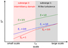 |
Fig. 8. Schematic illustration of the two subranges in the inertial regime of solar wind turbulence. Green, blue, and red lines represent Sq measured in the radial direction, and in the directions perpendicular and parallel to the local magnetic field, respectively. |
In this new scenario, the different scalings between the velocity and magnetic field could in fact be the result of the presence of two subranges. We note that the velocity has a smaller index than the magnetic field overall from the Wind observation. This could be the measurement effect as a consequence of the various non-Maxwellian ion distributions and instabilities in the solar wind (Verscharen et al. 2019; Bruno et al. 2024). Higher-resolution measurements could possibly confirm this conjecture.
The double power law phenomenon has already been discussed in both the 2D + slab model (Zank et al. 2020) and critical balance theory (Goldreich & Sridhar 1995; Howes et al. 2011). In the former framework, a double power law may appear with a Kolmogorov-like index in a smaller wavenumber regime dominated by quasi-2D fluctuations and an IK-like index in a larger wavenumber regime dominated by wave-like fluctuations. This prediction is in contrast to our results. In the latter case, there may exist a transitional scale beyond which weak wave turbulence drives itself into the critical balance regime. Such a transition is identified in a simulation of incompressible balanced decaying MHD turbulence (Meyrand et al. 2016) and in Earth’s magnetosheath (Zhao et al. 2024), which are both based on the change in the wavevector anisotropy obtained from wavelet spectrum analysis. However, we do not observe a transition of wavevector anisotropy, but a bloom of intermittency. The nature and generation of the intermittency should be further investigated in future studies. The transition scale also deserves future statistical study to provide clues as to why the transition occurs.
Note added in proof. Sioulas et al. (2022) analyzed magnetic field intermittency in the solar wind and found distinct features revealed by the multi-order structure functions for three different physical ranges in the inertial regime. Sioulas et al. (2023) investigated the radial evolution of power and spectral index anisotropy in the wavevector space of solar wind turbulence and also found the presence of two subranges within the inertial range from high-resolution analysis during the first perihelion of PSP. They compared their results with the results in our arXiv paper and proposed that the parallel spectral index in subrange 2 is steeper and closer to −2.
Acknowledgments
We acknowledge the members of Parker Solar Probe team, the Ulysses team and NASA’s Coordinated Data Analysis Web. We thank Linghua Wang and Qianyi Ma for helpful discussions. This work is supported by the National Natural Science Foundation of China under contract Nos. 42474203, 42104152, 41925018, 42174194, 42274213, 42474214. L.S.-V. was supported by the Swedish Research Council (VR) Research Grant N. 2022-03352 and by the International Space Science Institute (ISSI) in Bern, through ISSI International Team project #23-591 (Evolution of Turbulence in the Expanding Solar Wind).
References
- Badman, S. T., Bale, S. D., Oliveros, J. C. M., et al. 2020, ApJS, 246, 23 [Google Scholar]
- Bale, S. D., Goetz, K., Harvey, P. R., et al. 2016, Space Sci. Rev., 204, 49 [Google Scholar]
- Bale, S. D., Badman, S. T., Bonnell, J. W., et al. 2019, Nature, 576, 237 [NASA ADS] [CrossRef] [Google Scholar]
- Balogh, A., Beek, T. J., Forsyth, R. J., et al. 1992, A&AS, 92, 221 [NASA ADS] [Google Scholar]
- Biskamp, D. 2003, Magnetohydrodynamic Turbulence (Cambridge: Cambridge University Press) [Google Scholar]
- Boldyrev, S. 2006, Phys. Rev. Lett., 96, 115002 [Google Scholar]
- Bruno, R., & Carbone, V. 2013, Liv. Rev. Sol. Phys., 10, 2 [Google Scholar]
- Bruno, R., De Marco, R., D’Amicis, R., et al. 2024, ApJ, 969, 106 [NASA ADS] [CrossRef] [Google Scholar]
- Case, A. W., Kasper, J. C., Stevens, M. L., et al. 2020, ApJS, 246, 43 [Google Scholar]
- Chen, C. H. K., Mallet, A., Schekochihin, A. A., et al. 2012, ApJ, 758, 120 [Google Scholar]
- Chen, C. H. K., Bale, S. D., Bonnell, J. W., et al. 2020, ApJS, 246, 53 [Google Scholar]
- Chhiber, R., Matthaeus, W. H., Bowen, T. A., & Bale, S. D. 2021, ApJ, 911, L7 [NASA ADS] [CrossRef] [Google Scholar]
- Coleman, P. J. 1968, ApJ, 153, 371 [Google Scholar]
- Dudok de Wit, T. 2004, Phys. Rev. E, 70, 055302 [Google Scholar]
- Dudok de Wit, T., Krasnoselskikh, V. V., Bale, S. D., et al. 2020, ApJS, 246, 39 [Google Scholar]
- Forman, M. A., Wicks, R. T., & Horbury, T. S. 2011, ApJ, 733, 76 [Google Scholar]
- Fox, N. J., Velli, M. C., Bale, S. D., et al. 2016, Space Sci. Rev., 204, 7 [Google Scholar]
- Goldreich, P., & Sridhar, S. 1995, ApJ, 438, 763 [Google Scholar]
- Greco, A., Matthaeus, W. H., Perri, S., et al. 2018, Space Sci. Rev., 214, 1 [NASA ADS] [CrossRef] [Google Scholar]
- Horbury, T. S., Balogh, A., Forsyth, R. J., & Smith, E. J. 1996, A&A, 316, 333 [NASA ADS] [Google Scholar]
- Horbury, T. S., Forman, M., & Oughton, S. 2008, Phys. Rev. Lett., 101, 175005 [Google Scholar]
- Hossain, M., Gray, P. C., Pontius, D. H., Matthaeus, W. H., & Oughton, S. 1995, Phys. Fluids, 7, 2886 [NASA ADS] [CrossRef] [Google Scholar]
- Howes, G. G., Tenbarge, J. M., & Dorland, W. 2011, Phys. Plasmas, 18, 102305 [NASA ADS] [CrossRef] [Google Scholar]
- Huang, S. Y., Xu, S. B., Zhang, J., et al. 2022, ApJ, 929, L6 [Google Scholar]
- Iroshnikov, P. S. 1964, Soviet Astron., 7, 566 [Google Scholar]
- Kasper, J. C., Abiad, R., Austin, G., et al. 2016, Space Sci. Rev., 204, 131 [Google Scholar]
- Kasper, J. C., Bale, S. D., Belcher, J. W., et al. 2019, Nature, 576, 228 [Google Scholar]
- Kolmogorov, A. 1941, Dokl. Akad. Nauk SSSR, 30, 301 [NASA ADS] [Google Scholar]
- Kraichnan, R. H. 1965, Phys. Fluids, 8, 1385 [Google Scholar]
- Lepping, R. P., Acũna, M. H., Burlaga, L. F., et al. 1995, Space Sci. Rev., 71, 207 [Google Scholar]
- Lin, R. P., Anderson, K. A., Ashford, S., et al. 1995, Space Sci. Rev., 71, 125 [CrossRef] [Google Scholar]
- Linkmann, M. F., Berera, A., McComb, W. D., & McKay, M. E. 2015, Phys. Rev. Lett., 114, 235001 [Google Scholar]
- Lithwick, Y., Goldreich, P., & Sridhar, S. 2007, ApJ, 655, 269 [Google Scholar]
- Marino, R., & Sorriso-Valvo, L. 2023, Phys. Rep., 1006, 1 [NASA ADS] [CrossRef] [Google Scholar]
- Marino, R., Sorriso-Valvo, L., D’Amicis, R., et al. 2012, ApJ, 750, 41 [NASA ADS] [CrossRef] [Google Scholar]
- Matteini, L., Horbury, T. S., Neugebauer, M., & Goldstein, B. E. 2014, Geophys. Res. Lett., 41, 259 [Google Scholar]
- Matthaeus, W. H., Goldstein, M. L., & Roberts, D. A. 1990, J. Geophys. Res., 95, 20673 [Google Scholar]
- Meyrand, R., Galtier, S., & Kiyani, K. H. 2016, Phys. Rev. Lett., 116, 105002 [NASA ADS] [CrossRef] [Google Scholar]
- Mondal, S., Banerjee, S., & Sorriso-Valvo, L. 2025, ApJ, 982, 199 [Google Scholar]
- Monin, A. S., & Yaglom, A. M. 1975, Statistical Fluid Mechanics: Mechanics of Turbulence. Volume 2/Revised (Cambridge: MIT Press) [Google Scholar]
- Osman, K. T., Kiyani, K. H., Chapman, S. C., & Hnat, B. 2014, ApJ, 783, L27 [CrossRef] [Google Scholar]
- Oughton, S., & Matthaeus, W. H. 2020, ApJ, 897, 37 [Google Scholar]
- Pei, Z., He, J., Wang, X., et al. 2016, J. Geophys. Res., 121, 911 [Google Scholar]
- Podesta, J. J. 2009, ApJ, 698, 986 [NASA ADS] [CrossRef] [Google Scholar]
- Podesta, J. J., Roberts, D. A., & Goldstein, M. L. 2007, ApJ, 664, 543 [NASA ADS] [CrossRef] [Google Scholar]
- Politano, H., & Pouquet, A. 1998, Phys. Rev. E, 57, R21 [CrossRef] [Google Scholar]
- Salem, C., Mangeney, A., Bale, S. D., & Veltri, P. 2009, ApJ, 702, 537 [Google Scholar]
- Schekochihin, A. A., & Cowley, S. C. 2007, in Magnetohydrodynamics: Historical Evolution and Trends, eds. S. Molokov, R. Moreau, & H. K. Moffatt, 85 [Google Scholar]
- Schekochihin, A. A., Cowley, S. C., Taylor, S. F., Maron, J. L., & McWilliams, J. C. 2004, ApJ, 612, 276 [NASA ADS] [CrossRef] [Google Scholar]
- Sioulas, N., Huang, Z., Velli, M., et al. 2022, ApJ, 934, 143 [CrossRef] [Google Scholar]
- Sioulas, N., Velli, M., Huang, Z., et al. 2023, ApJ, 951, 141 [CrossRef] [Google Scholar]
- Sioulas, N., Zikopoulos, T., Shi, C., et al. 2024, ArXiv e-prints [arXiv:2404.04055] [Google Scholar]
- Smith, C. W., Matthaeus, W. H., Zank, G. P., et al. 2001, J. Geophys. Res., 106, 8253 [Google Scholar]
- Smith, C. W., Isenberg, P. A., Matthaeus, W. H., & Richardson, J. D. 2006a, ApJ, 638, 508 [Google Scholar]
- Smith, C. W., Hamilton, K., Vasquez, B. J., & Leamon, R. J. 2006b, ApJ, 645, L85 [NASA ADS] [CrossRef] [Google Scholar]
- Sorriso-Valvo, L., Marino, R., Foldes, R., et al. 2023, A&A, 672, A13 [NASA ADS] [CrossRef] [EDP Sciences] [Google Scholar]
- Taylor, G. I. 1938, Proc. R. Soc. London Ser. A: Math. Phys. Eng. Sci., 164, 476 [Google Scholar]
- Telloni, D. 2022, Front. Astron. Space Sci., 9, 917393 [NASA ADS] [CrossRef] [Google Scholar]
- Telloni, D., Carbone, F., Bruno, R., et al. 2019, ApJ, 887, 160 [Google Scholar]
- Veltri, P. 1999, Plasma Phys. Control. Fusion, 41, A787 [Google Scholar]
- Verdini, A., & Grappin, R. 2015, ApJ, 808, L34 [NASA ADS] [CrossRef] [Google Scholar]
- Verscharen, D., Klein, K. G., & Maruca, B. A. 2019, Liv. Rev. Sol. Phys., 16, 5 [Google Scholar]
- von Karman, T., & Howarth, L. 1938, Proc. R. Soc. London Ser. A: Math. Phys. Eng. Sci., 164, 192 [Google Scholar]
- Wan, M., Oughton, S., Servidio, S., & Matthaeus, W. H. 2012, J. Fluid Mech., 697, 296 [NASA ADS] [CrossRef] [Google Scholar]
- Wang, X., Tu, C., He, J., Marsch, E., & Wang, L. 2014, ApJ, 783, L9 [NASA ADS] [CrossRef] [Google Scholar]
- Wicks, R. T., Horbury, T. S., Chen, C. H. K., & Schekochihin, A. A. 2010, MNRAS, 407, L31 [Google Scholar]
- Wicks, R. T., Horbury, T. S., Chen, C. H. K., & Schekochihin, A. A. 2011, Phys. Rev. Lett., 106, 045001 [Google Scholar]
- Wu, H., Tu, C., Wang, X., et al. 2020, ApJ, 892, 138 [Google Scholar]
- Wu, H., Huang, S., Wang, X., Yang, L., & Yuan, Z. 2023a, ApJ, 958, L28 [Google Scholar]
- Wu, H., Huang, S., Wang, X., et al. 2023b, ApJ, 947, L22 [Google Scholar]
- Zank, G. P., Nakanotani, M., Zhao, L. L., Adhikari, L., & Telloni, D. 2020, ApJ, 900, 115 [Google Scholar]
- Zhao, S., Yan, H., Liu, T. Z., Yuen, K. H., & Wang, H. 2024, Nat. Astron., 8, 725 [Google Scholar]
All Figures
|
Fig. 1. Time series of three components of magnetic field (blue) in RTN coordinates and the flow speed (black) for the Ulysses interval (left) and the PSP interval (right). The dashed red lines denote the speed of 500 km/s. The time is indicated as year-month-day, in UTC for the Ulysses interval and as hour-minutes-seconds, in UTC for the PSP interval. |
| In the text | |
|
Fig. 2. Structure functions and scaling indices of magnetic field in the fast solar wind at 1.48 au observed by Ulysses. (a)–(c) Sq versus τ (bottom axis) and L (upper axis, in unit of the ion inertial length, di) measured in the radial direction, and in the directions perpendicular and parallel to the local magnetic field, respectively. The blue, orange, green, red, and purple represent Sq of order q = 1, 2, 3, 4, 5, respectively. The dashed yellow and cyan lines are power-law fits to Sq in subranges 1 and 2, shown with red and black shadows, respectively. (d)–(f) ξ(q), ξ⊥(q), ξ∥(q). The black and red represent the results in subrange 1 and 2, respectively. The horizontal dashed lines denote ξ = 1/2, 2/3, 1, respectively. The standard errors of these indices are small and no larger than the size of the markers. |
| In the text | |
|
Fig. 3. Structure functions and the scaling indices in the slow solar wind at 0.17 au observed by PSP. (a) Sq for the magnetic field measured in the radial direction with the same formats as Fig. 2. (b) ξ(q) for both the magnetic field (triangles) and velocity (squares) obtained from PSP and for the magnetic field (circles) obtained from Ulysses. The black and red represent the results in subrange 1 and 2, respectively. The horizontal dashed lines denote ξ = 1/2 and ξ = 2/3. |
| In the text | |
|
Fig. 4. Averaged scaling indices of magnetic field versus the order measured by Wind in the radial direction (a), and in the directions perpendicular (b) and parallel (c) to the local magnetic field. The stars (dots) denote the results from Wind (Ulysses). The black and red represent the results in subrange 1 and 2. The horizontal dashed lines denote ξ = 1/2, 2/3, 1, respectively. The standard errors of these indices are shown by error bars. |
| In the text | |
|
Fig. 5. Top: Count distribution of the second-order scaling indices for magnetic field measured by Wind in the radial direction (a), and in the directions perpendicular (b) and parallel (c) to the local magnetic field. Black and red denote subranges 1 and 2. The top right corners show the averages with their standard deviations. Bottom: Distribution of the second-order scaling indices of velocity in the same format as the top panels. |
| In the text | |
|
Fig. 6. (a) Second-order structure functions of magnetic field for the Ulysses interval. Black and red shadows denote subranges 1 and 2. Blue and red dots represent S2(τ⊥) and S2(τ∥). The numbers with the colors show the power law fit indices for the corresponding dots and the dashed lines with these indices are plotted to guide the eye. Inset: k∥ versus k⊥ for the same S2 level. (b) Mixed third-order structure functions Y for the PSP interval. The linear fit in subrange 1 is shown by dashed lines, which are used to evaluate the cascade rates. Inset: Y+ (blue) and Y− (red). |
| In the text | |
|
Fig. 7. Percentage of the intermittency for the Ulysses interval. Green, blue, and red represent the measurements in the radial direction, and in the directions perpendicular and parallel to the local magnetic field, respectively. |
| In the text | |
|
Fig. 8. Schematic illustration of the two subranges in the inertial regime of solar wind turbulence. Green, blue, and red lines represent Sq measured in the radial direction, and in the directions perpendicular and parallel to the local magnetic field, respectively. |
| In the text | |
Current usage metrics show cumulative count of Article Views (full-text article views including HTML views, PDF and ePub downloads, according to the available data) and Abstracts Views on Vision4Press platform.
Data correspond to usage on the plateform after 2015. The current usage metrics is available 48-96 hours after online publication and is updated daily on week days.
Initial download of the metrics may take a while.