| Issue |
A&A
Volume 686, June 2024
|
|
|---|---|---|
| Article Number | A28 | |
| Number of page(s) | 9 | |
| Section | The Sun and the Heliosphere | |
| DOI | https://doi.org/10.1051/0004-6361/202348573 | |
| Published online | 27 May 2024 | |
Preferential acceleration of heavy ions in magnetic reconnection: Hybrid-kinetic simulations with electron inertia
1
Zentrum für Astronomie und Astrophysik, Technische Universität Berlin, Hardenbergstr. 36, 10623 Berlin, Germany
e-mail: This email address is being protected from spambots. You need JavaScript enabled to view it.
2
Astronomical Institute of the Academy of Sciences of the Czech Republic, Friova 298, Ondejov 251 65, Czech Republic
3
Southwest Research Institute, 6220 Culebra Road, San Antonio, TX 78238, USA
Received:
12
November
2023
Accepted:
12
February
2024
Abstract
Context. Solar energetic particles (SEPs) in the energy range 10 s KeV nucleon−1–100s MeV nucleon−1 originate from the Sun. Their high flux near Earth may damage the space-borne electronics and generate secondary radiation that is harmful for life on Earth. Thus, understanding their energization on the Sun is important for space weather prediction. Impulsive (or 3He-rich) SEP events are associated with the acceleration of charge particles in solar flares by magnetic reconnection and related processes. The preferential acceleration of heavy ions and the extraordinary abundance enhancement of 3He in the impulsive SEP events are not understood yet.
Aims. In this paper we study the acceleration of heavy ions and its consequences for their abundance enhancements by magnetic reconnection, an established acceleration source for impulsive SEP events in which heavy-ion enhancement is observed
Methods. We employed a two-dimensional hybrid-kinetic plasma model (kinetic ions and inertial electron fluid) to simulate magnetic reconnection. All the ion species are treated self-consistently in our simulations.
Results. We find that heavy ions are preferentially accelerated to energies many times higher than their initial thermal energies by a variety of acceleration mechanisms operating in reconnection. The most efficient acceleration takes place in the flux pileup regions of magnetic reconnection. Heavy ions with sufficiently low values of charge-to-mass ratio (Q/M) can be accelerated by pickup mechanism in outflow regions even before any magnetic flux is piled up. The energy spectra of heavy ions develop a shoulder-like region, a nonthermal feature, as a result of the acceleration. The spectral index of the power-law fit to the shoulder region of the spectra varies approximately as (Q/M)−0.64. The abundance enhancement factor, defined as the number of particles above a threshold energy normalized to the total number of particles, scales as (Q/M)−α, where α increases with the energy threshold. We discuss our simulation results in the light of the SEP observations.
Key words: Sun: corona / Sun: flares / Sun: magnetic fields / solar wind
© The Authors 2024
 Open Access article, published by EDP Sciences, under the terms of the Creative Commons Attribution License (https://creativecommons.org/licenses/by/4.0), which permits unrestricted use, distribution, and reproduction in any medium, provided the original work is properly cited.
This article is published in open access under the Subscribe to Open model. This email address is being protected from spambots. You need JavaScript enabled to view it. to support open access publication.
1. Introduction
Nonthermal acceleration of charged particles is a widespread process in space and astrophysical plasmas ranging from planetary magnetospheres to clusters of galaxies. The accelerated particles, mostly ions, are detected near and on Earth in a wide energy range, 104 − 1020 eV, either directly by particle detectors on satellites and high-altitude balloons or indirectly by detecting the secondary particles and electromagnetic radiation produced by their interaction with Earth’s atmosphere. These particles are generally categorized as solar energetic particles (SEPs), galactic cosmic rays, and extra-galactic cosmic rays based on their source regions in our star the Sun, our Galaxy the Milky Way, and beyond our Galaxy, respectively. SEPs in a typical energy range of 10 s KeV nucleon−1–100 s MeV nucleon−1 are of particular interest because their flux near Earth is sufficiently high to have implications for space weather phenomena.
Solar energetic particle events can be classified into impulsive events (short duration ≤ 1 day; less intense, smaller particle fluxes with typical energies < 10 MeV nucleon−1; and numerous, about 1000 per year) and gradual events (long duration, several days; orders of magnitude more intense, large particle fluxes with energies > 10 MeV nucleon−1; less frequent ∼ 10 per year) (Reames 1999, 2021b). Gradual events are attributed to the acceleration of charged particles by coronal mass ejection (CME) driven shocks, while impulsive events are attributed to the acceleration in solar flares by magnetic reconnection and associated processes (Kahler et al. 2001; Mason 2007; Drake et al. 2009; Lin 2011; Reames 2013, 2022; Murphy et al. 2016; Desai & Giacalone 2016; Bučík 2020). Impulsive events show abundance enhancements of heavier ions relative to their abundances in the solar corona at energies well above their average thermal energy (∼100 eV) (Reames 2021a). In contrast, the average abundances of elements in gradual events are similar to those in solar corona (e.g., Reames 2018). The enhancement factor, defined as the ratio of the relative (to a reference element, usually oxygen) abundances of an element X in impulsive SEP events and solar corona, exhibits power-law dependence on an ion’s charge (Q) to mass (M) ratio as (Q/M)−α for M ≥ 4 amu. Variations in the value of α have been found from event to event (Reames et al. 2014b) with mean values α = 3.26 (at 0.375 MeV nucleon−1; Mason et al. 2004), α = 3.64 ± 0.15 (at 3–10 MeV nucleon−1; Reames et al. 2014a), α = 3.53 (at 160–226 KeV nucleon−1), and α = 3.31 (at 320–453 KeV nucleon−1; Bučík et al. 2021). The enhancement factor for the 3He isotope, however, does not obey the power law and can have very large values (up to 104) compared to those calculated using the power law (Kocharov & Kocharov 1984; Mason 2007). For this reason, impulsive SEP events are also called 3He-rich events. However, the enhancement of heavy ions is not correlated with the extraordinary enhancement of 3He (Mason et al. 1986; Reames 1999).
The abundance enhancements of heavy ions with low values of Q/M and the extraordinary abundance enhancement of 3He in impulsive SEP events are not understood yet. Since these enhancements are uncorrelated (Mason et al. 1986; Reames 1999), attempts have been made to explain the abundance enhancement of heavy ions and 3He by separate mechanisms. Abundance enhancement of heavy ions is thought to be due to their preferential acceleration by magnetic reconnection and the associated processes in solar flares from thermal to SEP energies. Models of the preferential acceleration of heavy ions consider resonant interaction of the ions with the waves in Alfvénic plasma turbulence (Miller 1998; Eichler 2014; Kumar et al. 2017; Fu et al. 2020; Shi et al. 2022) that may be generated during magnetic reconnection, for example the development of turbulent outflows, as shown by fully kinetic 3D simulations of magnetic reconnection (Lapenta et al. 2020). Turbulent energy decays with wave frequency, which means that higher frequency waves have lower energy. Heavy ions with lower values of Q/M have lower values of cyclotron frequency (∝Q/M), and thus would resonate with lower frequency but higher power waves in turbulence, favoring the preferential acceleration of heavy ions. In addition, turbulence amplitudes above a threshold can make ion orbits chaotic, thus heating ions stochastically. Phenomenological arguments and simulations of test particles interacting with turbulent spectra of Alfvén and kinetic Alfvén waves at wavelengths comparable to ion gyro-radius in plasmas with β < 1 found that, at comparable temperatures, alpha particles and heavier ions are stochastically heated more efficiently than the protons (Chandran et al. 2010). Three-dimensional hybrid-kinetic simulations of continuously driven Alfvénic turbulence at low plasma beta show that the Hall and thermoelectric effects in a generalized Ohm’s law contribute significantly to the stochastic ion heating, which is enhanced by the intermittency in the turbulence (Cerri et al. 2021). The mechanisms proposed for the preferential acceleration of 3He consider absorption of some wave energy by cyclotron resonance of 3He with the wave (Fisk 1978; Temerin & Roth 1992; Liu et al. 2006). These waves can be produced by electron beams, for example by electrons streaming along open magnetic field lines in solar corona, or via coupling with low-frequency Alfvén waves. Efficient acceleration of 3He by ion-cyclotron resonance has been observed in nuclear fusion devices, which has implications for space plasmas as well (Kazakov et al. 2017).
Magnetic reconnection can also accelerate electrons and ions in solar flares by nonresonant mechanisms, which have also been considered to explain the preferential acceleration of heavy ions (Drake et al. 2009; Bárta et al. 2011b,a; Zhou et al. 2015, 2016). In 2.5D magnetohydrodynamic (MHD) and test particle simulations (Kramoliš et al. 2022), heavy ions were found to be preferentially accelerated by first-order Fermi processes in cascading plasmoids generated by spontaneous magnetic reconnection in a meso-scale current sheet. The ion energy spectra and abundance enhancement factors exhibit power-law profiles. The index of the power law for the abundance enhancement factor, however, was not in agreement with the observations. The authors suspected that the disagreement could be due to the limitation of the MHD model, which lacks the kinetic physics essential for magnetic reconnection in collisionless plasmas. In 2D fully kinetic simulations of magnetic reconnection, ions entering the reconnection exhaust can behave like pickup particles and can be accelerated if their Q/M is below a threshold value, resulting in the preferential acceleration of heavy ions. An explanation for the power-law dependence of the enhancements on Q/M was proposed based on the pickup mechanism (Drake et al. 2009; Knizhnik et al. 2011). These simulations, carried out only for one ion species (4He2+), did not verify the power-law dependence. Therefore, it is not clear whether the acceleration of heavy ions by pickup mechanisms can provide the observed scaling of the abundance enhancement with Q/M. Magnetic reconnection in turbulence generated current sheets, which form in turbulence as a result of the magnetic energy cascade from large to kinetic scales where magnetic fluctuations have intermittent statistics (Cerri et al. 2019), have also been suggested to contribute to the energization of charged particles (Rueda et al. 2022; Grošelj et al. 2017).
Magnetic reconnection in collisionless plasmas is a multi-scale process that occurs at electron kinetic scales and then couples to ion scales and even larger macro-scales. An ideal simulation of magnetic reconnection requires the kinetic treatment of electrons and ions and covering scales from electron kinetic scales all the way up to large macro-scales well above the ion kinetic scales. Such fully kinetic simulations (e.g., using the particle-in-cell, PIC, method) of magnetic reconnection in electron-proton plasma are computationally very demanding. The self-consistent inclusion of heavier ion species make the simulations even more demanding because now it is necessary to use a larger simulation box to accommodate the larger gyro-radii of the heavier species, while at the same time resolving the electron scales. For this reason a variety of reduced kinetic models have been used for numerical studies of magnetic reconnection, plasma turbulence, and the associated charge particle heating. Plasma turbulence at ion scale was studied using hybrid-kinetic simulations (with and without electron inertia) along with fully kinetic simulations (Cerri et al. 2019). Two-dimensional fully kinetic, gyro-kinetic, and hybrid-kinetic simulations of plasma turbulence suggest that magnetic reconnection can heat electrons and ions in turbulence generated current structures (Grošelj et al. 2017). Three-dimensional hybrid-kinetic simulations of driven Alfvén-wave turbulence show a flattened core in the perpendicular-velocity distribution and non-Maxwellian wings in the parallel-velocity distribution of ions resulting from the dissipation of kinetic Alfvén waves at sub-ion scales (Arzamasskiy et al. 2019). Two-dimensional simulations of guide field magnetic reconnection by means of a hybrid-Vlasov-Landau-fluid (HVLF) model reproduces the main features of magnetic reconnection and anisotropic heating of electrons (Finelli et al. 2021). In hybrid-kinetic simulations (with massless electron fluid) of plasma turbulence, preferential heating of alpha particles with respect to protons was observed near current sheets in spatial regions of enhanced ion vorticity (Valentini et al. 2016).
In this paper, we employ 2D hybrid-kinetic simulations (kinetic ions and inertial electron fluid) to study the acceleration of heavy ions and its consequences for their abundance enhancements by magnetic reconnection, an established acceleration source for impulsive SEP events in which heavy-ion enhancement is observed (Kahler et al. 2001; Mason 2007; Drake et al. 2009; Lin 2011; Murphy et al. 2016; Reames 2022). Treatment of electrons as an inertial fluid allows inclusion of the physics at electron inertial scale, but relaxes the numerical requirement of resolving the Debye length in the PIC method, and therefore allows larger simulation domains for the same number of grid points. The computational feasibility, however, comes at the cost of electron kinetic physics, which is acceptable as long as the study of the ion acceleration is the primary objective. All the ion species are treated self-consistently in our simulations. We use the term “heavy ion” to mean any ion species whose mass M is higher than the proton’s mass. The paper is organized as follows. Section 2 presents the simulation setup. The simulation results are presented in Sect. 3, and are discussed and concluded in Sect. 4.
2. Simulation setup
We carried out 2D hybrid-kinetic simulations of magnetic reconnection with electron inertia using a hybrid-PIC code called “Code Hybrid with Inertial Electron Fluid (CHIEF)”, which is a 3D parallelized code based on message passing interface (MPI) for high-performance computing (Muñoz et al. 2018, 2023; Jain et al. 2022). In the hybrid code CHIEF, electrons are treated as an inertial and isothermal fluid whose equations are coupled to Maxwell’s equation to obtain the electric and magnetic fields. All the ions (protons and heavier ions), on the other hand, are treated self-consistently as kinetic species and their equations of motion in electric and magnetic fields are solved using the PIC method. The code CHIEF treats the inertial effects of the electron fluid without any of the approximations used by other electron-inertial hybrid-kinetic code (Jain et al. 2022). The details of the hybrid-kinetic model used in CHIEF, its numerical implementation and parallelization are discussed in our other publications (Muñoz et al. 2018, 2023; Jain et al. 2022).
We initialize the 2D simulations with two Harris current sheets, ![Mathematical equation: $ \mathbf{B}=\hat{z}B_{z0}[\tanh\{(\mathit{y}+L_{\mathit{y}}/4)/L\}-\tanh\{(\mathit{y}-L_{\mathit{y}}/4)/L\}-1]+\hat{x}B_{x0} $](/articles/aa/full_html/2024/06/aa48573-23/aa48573-23-eq1.gif) , in a y–z plane and a guide magnetic field Bx0 = 0.2 Bz0 perpendicular to the plane. The half-thickness L = dp of the current sheets is taken to be equal to a proton inertial length (dp) and Ly is the length of the simulation domain along the y-direction. A small initial perturbation is added to the Harris equilibrium to form an X-point and an O-point in the current sheets centered at y = −Ly/4 and y = Ly/4, respectively. The plasma of Harris current sheets consists of quasi-neutral populations of proton particles and electron fluid with Harris equilibrium density profile ne = np = n0[sech2{(y + Ly/4)/L}+sech2{(y − Ly/4)/L}]. Harris sheets are embedded in a uniform background plasma of density 0.2 n0 and therefore peak density at their centers is 1.2 n0. The background plasma consists of electron fluid and particle populations of heavy ions (only one species) and protons with densities nbe = 0.2 n0, nbi = 0.01 n0 (5% of the background plasma density), and nbp = nbe − Z nbi, respectively, where Z is the charge state of heavy ions with charge of heavy ion species given by Q = Z e. The initial velocity distribution of the protons and heavy ions is Maxwellian. The initial temperatures of electrons, protons, and heavy ions are the same:
, in a y–z plane and a guide magnetic field Bx0 = 0.2 Bz0 perpendicular to the plane. The half-thickness L = dp of the current sheets is taken to be equal to a proton inertial length (dp) and Ly is the length of the simulation domain along the y-direction. A small initial perturbation is added to the Harris equilibrium to form an X-point and an O-point in the current sheets centered at y = −Ly/4 and y = Ly/4, respectively. The plasma of Harris current sheets consists of quasi-neutral populations of proton particles and electron fluid with Harris equilibrium density profile ne = np = n0[sech2{(y + Ly/4)/L}+sech2{(y − Ly/4)/L}]. Harris sheets are embedded in a uniform background plasma of density 0.2 n0 and therefore peak density at their centers is 1.2 n0. The background plasma consists of electron fluid and particle populations of heavy ions (only one species) and protons with densities nbe = 0.2 n0, nbi = 0.01 n0 (5% of the background plasma density), and nbp = nbe − Z nbi, respectively, where Z is the charge state of heavy ions with charge of heavy ion species given by Q = Z e. The initial velocity distribution of the protons and heavy ions is Maxwellian. The initial temperatures of electrons, protons, and heavy ions are the same:  , where mp is proton mass and
  is the proton Alfvén velocity based on Bz0 and n0.
Each of our simulations consists of only one species of heavy ion. We consider the following four different species of heavy ions to be included (one at a time) in our simulations: 4He2+, 3He2+, 16O7+, and 56Fe14+. We take the proton-to-electron mass ratio as mp/me = 25. The simulation domain Ly × Lz is 51.2 dp × 102.4 dp resolved by a grid spacing of 0.1 dp in each direction. The time step is  , where ωcp = eBz0/mp is the proton cyclotron frequency. We take 500 and 200 particles per cell for protons and heavy ions, respectively. Plasma resistivity is taken to be zero and electron inertia allows the magnetic reconnection. Boundary conditions are periodic.
3. Simulation results
Figure 1 shows the evolution of the out-of-plane current density Jx from the initial to the late phase. In the initial phase (ωcpt = 19.6), an X-point forms in the lower current sheet (y < 0), while an O-point forms in the upper current sheet (y > 0), as per the initialized perturbation. By ωcpt = 39.19, the lower and the upper current sheets spontaneously develop magnetic islands as a result of magnetic reconnection at multiple sites, even though the initialized perturbation was chosen to initiate reconnection at a single site in the simulation domain. The magnetic islands on each of the current sheets grow in size with time by merging and/or pushing among themselves and simultaneously develop turbulence inside them. At ωcpt = 58.79 the magnetic islands of the lower and upper current sheets grow to a big enough size that the particles accelerated in the upper (lower) current sheet may cross over to the lower (upper) current sheet.
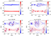 |
Fig. 1. Out-of-plane current density Jx/(n0eVAp) at four different times. |
Our objective here is to study the ion acceleration without the influence of the periodic boundaries. Since the upper current sheet is affected by the periodic boundary conditions along z-direction from the beginning (the initial X-points form at the z-boundaries), we focus on the lower current sheet for our studies. The lower current sheet is also likely to be affected by periodic boundaries along the z-direction after a time,  , Alfvén waves take to cross half the simulation domain. In order to avoid particles crossing from the upper half to the lower half of the simulation domain and the influence of periodic boundaries, we limit our analysis of results only up to the time ωcpt = 48.99 and in the spatial region −23 ≤ y/dp ≤ −3.
Figure 2a shows the evolution of fractional change in average kinetic energy from its initial value for different ion species. All the heavy ions gain energy first at slow rates up to ωcpt ≈ 30 after which they gain energy at much faster rates. We note that magnetic islands have significantly developed by ωcpt = 30. This can be seen in Fig. 2b, which shows that  (average of the magnetic energy in the normal component of the magnetic field along the central line of the lower current sheet, a proxy for the magnetic island development) begins to grow at ωcpt = 20, and by ωcpt = 30 has grown to ∼5% of the asymptotic magnetic energy in the anti-parallel magnetic field. The development of magnetic islands, therefore, seems to be linked with the efficient energization of heavy ions. Proton energization, on the other hand, does not seem to be affected significantly by the formation of magnetic islands as it does not enhance significantly after ωcpt ≈ 30.
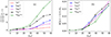 |
Fig. 2. Time development of the fractional change in average kinetic energy per particle, ⟨K.E.(t)⟩ptcl, from its initial value (a) and average of the square of the normal component of the magnetic field By along the central line of the lower current sheet (b) for different ion species. |
Heavier ions (16O7+ and 56O14+ in Fig. 2) get energized significantly in comparison to the lighter helium ions even during early phase of acceleration (0 < ωcpt < 30). This suggests that acceleration mechanisms, different from the mechanisms after ωcpt = 30, operate in the early phase only on the heavier ions, implying a threshold for the energization based on the heaviness of the ions. In order to understand the threshold behavior and the acceleration mechanisms before and after ωcpt = 30 (the time by which ∼5% of the magnetic energy of the asymptotic anti-parallel magnetic field has contributed to the development of magnetic islands), we show the locations of the energized particles in the reconnection region at ωcpt = 19.6 and 48.99 in two simulations, one with 4He2+ (Fig. 3) and the other with 16O7+ (Fig. 4). At ωcpt = 19.6, 16O7+ ions are more energized than 4He2+ ions and the locations of the energized 16O7+ ions are in the outflow regions. However, the energization is not uniformly distributed in the outflow regions: the energized particles are located near the upper (lower) separatrix in the left (right) outflow region. This observations combined with the threshold behavior of energization suggests the pick-up mechanism of the energization in which non-adiabatic ions are energized as they cross the reconnection separatrices (Drake et al. 2009). A threshold condition,  , for non-adibaticity of ions crossing the sepratrix in guide field reconnection was obtained by Drake et al. (2009), where mi and Zi = Qi/e are the mass and charge state of ions and βp is the proton plasma beta based on asymptotic value of the anti-parallel magnetic field. Although this condition, which becomes mi/Zimp > 1.12 for our simulation parameters, is satisfied by all the species of heavy ions we have considered, the 4He2+ and 3He2+ ions with mi/Zimp = 2 and 1.5 were not energized during ωcpt < 30.
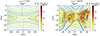 |
Fig. 3. Positions of 4He2+ ions represented by dots color-coded according to the ions’ kinetic energy at ωcpt = 19.6 (left column) and ωcpt = 48.99 (right column). The lines with arrows represent magnetic field lines. Only the lower half (y < 0) of the simulation domain is shown. |
It should be noted that the threshold condition was obtained assuming that the ions cross the separatrix with a velocity equal to 0.1vAp which is almost the upper bound on the inflow velocity in a fully developed steady-state magnetic reconnection (Liu et al. 2017). In our simulations, magnetic reconnection at ωcpt = 19.6 is still developing and the ion inflow velocity has not yet reached its maximum value. Using |uiy|≈0.05 vAp, the value of inflow velocity at ωcpt = 19.6 in our simulations, the threshold condition becomes mi/Zimp > 2.24, which allows non-adiabatic behavior for 56Fe14+ (mi/Zimp = 4) and only marginally for 16O7+ (mi/Zimp = 2.28), but not for 4He2+ (mi/Zimp = 2) and 3He2+ (mi/Zimp = 1.5).
The localization of energized 16O7+ ions near the upper (lower) separatrix in the left (right) outflow region at ωcpt = 19.6 is due to the asymmetries in the lower and upper separatrices in guide field magnetic reconnection (Pritchett & Coroniti 2004; Li & Zhang 2020). The thickness of the upper (lower) separatrix in the left (right) outflow region is smaller than that of the lower (upper) separatrix. This limits the non-adiabaticity, and thus the energization of ions entering the outflow regions from the thicker separatrix.
The increased rate of energization for all the heavy ion species after ωcpt = 30 is somehow linked to the growth of the normal component By of the magnetic field in the current sheet (Fig. 2). The normal component By in current sheet can grow large by nonsteady reconnection with increasing rate and/or the compression along the current sheet of the reconnected magnetic field lines. The compression can occur due to the pileup of the magnetic flux reconnected at two neighboring sites on the magnetic island between the two sites, contraction of magnetic islands and/or mutual pushing among magnetic islands. Several acceleration mechanisms may be associated with these scenarios: direct acceleration by inductive reconnection electric fields in the X-point regions, acceleration by motional electric fields induced by Alfvénic outflow in the outflow regions, Fermi-like acceleration in contracting magnetic islands, magnetic curvature and gradient drifts aligned with inductive or motional electric fields in the flux pileup regions, and betatron acceleration by time dependent magnetic fields in the flux compression regions.
Figures 3 and 4 show that, at ωcpt = 48.99, energized ions are located in the X-point regions, inside magnetic islands and outflow exhaust regions. Most energized particles (black dots in Figs. 3 and 4) are mostly concentrated near the opening of the exhaust regions, where the reconnected magnetic field lines usually pile up. In the case of simulations with 16O7+, the merging of two magnetic islands and the presence of energized ions at z ≈ 0 can also be seen (Fig. 4). Although the locations of the energetic particles at a given time are not necessarily in the neighborhood of their acceleration sites, it seems from Figs. 3 and 4 that a number of acceleration mechanisms out of those discussed above are operating simultaneously in different regions of reconnection. A given particle might experience acceleration due to different mechanisms it encounters on its trajectory in different reconnection regions. Disentangling these mechanisms requires a full history of the particles’ motion and therefore the tracking of their trajectories, and will be the subject of our future studies.
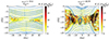 |
Fig. 4. Positions of 16O7+ ions represented by dots color-coded according to the ions’ kinetic energy at ωcpt = 19.6 (left column) and ωcpt = 48.99 (right column). The lines with arrows represent magnetic field lines. Only the lower half (y < 0) of the simulation domain is shown. |
Figure 5 shows the evolution of the energy spectra for different ions species. The energy spectra for all the ion species broaden with time. The energy spectra for protons did not develop any noticeable nonthermal features up to the final simulation time ωcpt = 48.99. Thus, the energy transferred to protons only heats them. A nonthermal feature, a shoulder in the spectra in the intermediate energy range after which spectra falls off rapidly, develops in the spectra of 4He2+ and 16O7+ at ωcpt = 39.19 and ωcpt = 19.6, respectively. The early development of the spectral shoulder for heavier ions, 16O7+ and 56Fe14+ (figure not shown), in comparison to the lighter ions, 4He2+ and 4He3+ (figure not shown), is consistent with the early energization of heavier ions by pickup mechanism. At ωcpt = 19.6, the energy of the accelerated 16O7+ (see Fig. 4) is in the range 1–10  at which 16O7+ spectra develop a shoulder. The spectral shoulder rises with time and extends to higher energies as more and more low-energy heavy ions are accelerated to higher energies.
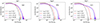 |
Fig. 5. Energy spectra of protons 1H1+ (a), 4He2+ (b), and 16O7+ (c) at different times. |
Figure 6a compares the energy-per-nucleon spectra of different ion species at ωcpt = 48.99, the last time up to which our simulations are valid. We note that, for the purpose of comparing the spectra of different ion species independent of their total mass, the spectra in Fig. 6a are shown as a function of energy-per-nucleon unlike the spectra in Fig. 5 which are shown as a function of energy. The injection energy  , around which the spectral shoulder begins, is similar for heavy ion species. The cutoff energy, up to which the shoulder extends, and the maximum gained energy per nucleon are higher for the lighter ion species. In Fig. 6b we plot the same spectra (excluding the proton spectra) as in Fig. 6a, but artificially shifted on the y-axis for better visibility of the spectral shoulder and power-law fits, Eγ, of the shoulder region of the spectra, where E is the energy-per-nucleon. The spectral indices of the fits, γ = −1.59, −1.53, and −1.68 respectively for 4He2+, 3He2+, and 16O7+ are quite similar. The spectra for 56Fe14+, on the other hand, are somewhat softer with γ = −3.0. The dependence of γ on Q/M, shown in Fig. 7a, can be approximately fitted as γ ∝ (Q/M)−0.64.
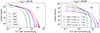 |
Fig. 6. Energy-per-nucleon spectra at ωcpt = 48.99. The original spectra of different ion species (a) and spectra of heavy ions shifted for visibility on the y-axis by a factor of 100, 101, 102, and 103 for 4He2+, 3He2+, 16O7+, and 56Fe14+, respectively (b). The dashed lines in the right panel are the power-law fit (Eγ) to the shoulder region of the spectra, where E is the energy-per-nucleon. |
In 3He-rich SEP events, ion abundances are enhanced relative to their solar abundances at energies well above their thermal energy. We consider a proxy for abundance enhancement factor F as number of particles above a threshold energy normalized to the total number of particles. Figure 7b shows this proxy of the abundance enhancement factor as a function of Q/M at ωcpt = 48.99 for three energy thresholds, Et = 10 KEth, 25 KEth, and 50 KEth, well above the initial thermal energy  , which is the same for all ion species in our simulations. The value of Et was chosen such that it is in the tail region of the initial energy spectra, which is the same for all the ion species and at the same time is not outside the shoulder regions of the energy spectra of the heavy ions at ωcpt = 48.99. Although the value
  is close to the cutoff energy of the shoulder region in the energy spectra of 4He2+ at ωcpt = 48.99 (see Fig. 5b), the abundances are dominated by the abundances in the shoulder region as the energy spectra falls off very rapidly beyond the shoulder region. We note that the threshold
  is in the rapidly falling region of the proton’s energy spectra at ωcpt = 48.99. It is acceptable, however, as the proton’s energy spectra does not develop a shoulder.
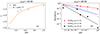 |
Fig. 7. Spectral index γ of the energy-per-nucleon spectra in the shoulder region vs. Q/M and the fit γ ∝ (Q/M)−0.64 (a). Scaling of the proxy of the ion abundance, defined as number of particles above a threshold energy normalized to the total number of particles, with Q/M for threshold energy 10 (red filled circles), 25 (blue plus signs), and 50 (black filled squares) times the initial thermal energy KEth (b). The straight lines are the fit, abundance ∝(Q/M)−α, for the data and are plotted with the color corresponding to the data. |
Figure 7b also shows the power-law fit F ∝ (Q/M)−α. The enhancement factor drops with increasing Q/M (i.e., heavier ions are preferentially accelerated). The drop in the enhancement factor becomes steeper (the value of α increases) with the increasing threshold energy. As the value of Et increases, the contribution of the shoulder region relative to the contribution of the rapidly falling region of the energy spectra toward the abundances decreases. This decrease in the contribution is more prominent for higher values of Q/M as the shoulder in their energy spectra extends to lower energies. This results in the increase in the value of α with Et.
4. Discussion and conclusion
We carried out hybrid-kinetic simulations (with electron inertia) to study the acceleration of heavy ions (Q/M < 1) by magnetic reconnection. We find that heavy ions can be accelerated to energies many times higher than their initial energies by a variety of acceleration mechanisms. Heavier ions are preferentially accelerated in the sense that energy gain averaged over particles increases with decreasing Q/M. They are primarily accelerated in magnetic islands and flux pileup regions near the opening of the outflow exhausts. The most efficient acceleration takes place in the flux pileup regions. Heavy ions, depending upon the low value of Q/M which allows them to be non-adiabatic while crossing from inflow to outflow regions, can also be accelerated by pickup mechanisms in outflow regions even before any magnetic flux is piled up. As a result of acceleration, heavy ions develop a shoulder, a nonthermal feature, in their energy spectra. The spectral index obtained from the power-law fit in the shoulder region of the spectra varies approximately as (Q/M)−0.64. The abundance enhancement factor, defined as the number of particles above a threshold energy normalized to the total number of particles, scales as (Q/M)−α, where α increases with the energy threshold.
Energy spectra with a shoulder or in other words double power law with a break in the spectra at energy ∼1 MeV nucleon−1 has been in situ observed in space (Mason et al. 2002; Bučík et al. 2018). Our simulations show the break in the energy spectra in the energy range 2–6  per nucleon, depending upon the ion species. The value of vAp in the active regions of solar corona, where acceleration takes place, has been estimated to lie in the range 2000–9000 km s−1 (Brooks et al. 2021). For a typical value vAp = 5000 km s−1,
  MeV, and therefore the break in the simulations occurs in the range 0.5–1.5 MeV nucleon−1, consistent with the observations. We note that the energy range of the break depends on the value of vAp, estimates of which in the solar corona vary significantly (Brooks et al. 2021). In the observations, the spectral index γ of the power law before the break is in the range 1–3 for the ions of helium-4, helium-3, oxygen, and iron. The values of γ before the break is in the same range in our simulations as well. The values of γ after the break are, however, much larger in our simulation than in the observations.
We defined a proxy F for the abundance enhancement factor to study its variation with Q/M. Although this proxy does not exactly correspond to the abundance enhancement factor used in observations, we point out some similarities and differences in the behavior of the two. In our simulations, the power-law index α of the fit F ∝ (Q/M)−α increases with the threshold energy. The observations also show variations from event to event in the value of α in the range −5 < α < 12 with a mean value of α = 3.26 at 385 keV nucleon−1 (Mason et al. 2004) and 2 < α < 8 with a mean value of α = 3.64 at 3–5 MeV nucleon−1 (Reames et al. 2014b,a). The mean values in the observations are similar, even though their energies are an order of magnitude apart. The mean of the three values of α obtained from power-law fits in Fig. 7b is approximately 3.66. In observations, steeper energy spectra tend to have a steeper fall in the abundance enhancement with Q/M (i.e., a large value of α; Reames et al. 2014b). This effect is similar to the increase in the value of α with Et in our simulations. Larger values of Et increases the contribution of the steeper part of the energy spectra in the calculations of the abundances.
Our simulations consider only a single species of heavy ions at a time. In a physical situation, multiple heavy ion species will be present in reconnection regions at the same time and accelerated simultaneously by magnetic reconnection, partitioning the available magnetic energy among the species. This can affect the maximum energy gained by a given species, but is unlikely to affect the preferential acceleration of heavy ions, at least as long as the heavy ions are minor species (in the solar corona heavy ions with Z > 2 compose only 0.1% of all ions while helium is 8.9%; Lodders 2019) so that the electric and magnetic field in the reconnection region are mainly due to the electron and proton dynamics with only a small contribution from the heavy ion species. However, simulations of magnetic reconnection with multiple heavy ion species are required to understand if the minority species can influence the accelerating fields and, if so, to what extent.
It should be noted that the SEP events are detected in space far away from their acceleration sites on Sun. The observed scaling of abundance enhancement with Q/M and other features of these events may therefore not necessarily be the effect of acceleration alone, but also of the transport of particles from the acceleration site to the detection site. In fact, 3D test particle modeling of the inter-planetary transport of relativistic protons from the source region on the Sun shows that the spectra of the particles is highly observer dependent and do not necessarily reflect the source spectra (Dalla et al. 2020). These transport effects are possible for the spectra of heavy ions as well. However, observations of impulsive events (their intensity time profiles, velocity dispersion, and anisotropies) indicate their nearly scatter-free propagation with scattering mean free paths > 1 au (e.g., Reames 2020, 2022) and therefore a direct comparison with acceleration models is meaningful (Mason et al. 2002 and references therein). The authors point out that while the effects of interplanetary propagation on these events are not large, a definitive resolution requires observations close to the Sun.
We conclude that magnetic reconnection is a potential candidate for the preferential acceleration of heavy ions, which may provide a power-law dependence of the abundance enhancement on Q/M, as suggested by the results presented here. More detailed studies on the relative roles of the different acceleration mechanisms operating in magnetic reconnection in the abundance enhancement will be presented in a future publication. We note that we did not find any extraordinary abundance enhancement of 3He2+ in our simulations. This, however, does not rule out the role of magnetic reconnection in the abundance enhancement of 3He2+ as our simulations are carried out only for limited range of parameters and in two dimensions. Magnetic reconnection in three dimensions is host to a number of additional three-dimensional instabilities and allows more complex interactions in the reconnection region. For example, flux ropes formed by the growth of a 3D oblique plasmoid instability in a low-beta reconnecting current layer undergo complex interactions due to the advection and rotation by the reconnection outflow jets, leading to a turbulent state with a stochastic magnetic field and the development of secondary flux ropes in thin current layers that form between the primary flux-ropes (Stanier et al. 2019). A finite guide magnetic field on the order of the reconnecting component and axial structure of flux ropes in 3D magnetic reconnection enable efficient electron acceleration by allowing the particles to leak out and return to acceleration regions, as shown by 3D kinetic simulations (Dahlin et al. 2017). Fully kinetic simulations show that electron acceleration by parallel electric field and curvature driven mechanisms can be enhanced by the filamentation of electric and magnetic fields caused by streaming instabilities in the nonlinear stage of 3D guide-field magnetic reconnection (Muñoz & Büchner 2018). Strong drift-wave fluctuations in the lower-hybrid frequency range, developed in fully kinetic 3D simulations of asymmetric magnetic reconnection (modeling MMS magnetopause diffusion region crossings), give rise to cross-field electron transport and significantly enhanced electron parallel heating in comparison to 2D simulations (Le et al. 2018). It seems likely that 3D plasma instabilities in magnetic reconnection will interact with 3He2+ and other heavy ions as well and contribute to their acceleration, as they do for electron acceleration. The details of these complex interactions are unknown and are the subjects for further studies.
Acknowledgments
The authors thank Patricio Muñoz for fruitful discussion and his help. We gratefully acknowledge the financial support by the German Science Foundation (DFG), projects JA 2680-2-1 and BU 777-17-1 as well as the Czech Republic GAĈR project 20-09922J M, personally Markus Rampp and Meisam Tabriz of the Max Planck Computing and Data Facility (MPCDF) for their support of the development of the hybrid-kinetic code CHIEF used for the simulation studies presented in this paper. The simulations were carried out on the MPS supercomputers at the MPCDF, Garching, Germany. R.B. acknowledges support by NASA grants 80NSSC21K1316 and 80NSSC22K0757.
References
- Arzamasskiy, L., Kunz, M. W., Chandran, B. D. G., & Quataert, E. 2019, ApJ, 879, 53 [NASA ADS] [CrossRef] [Google Scholar]
- Bárta, M., Büchner, J., Karlický, M., & Kotrč, P. 2011a, ApJ, 730, 47 [CrossRef] [Google Scholar]
- Bárta, M., Büchner, J., Karlický, M., & Skála, J. 2011b, ApJ, 737, 24 [CrossRef] [Google Scholar]
- Brooks, D. H., Warren, H. P., & Landi, E. 2021, ApJ, 915, L24 [NASA ADS] [CrossRef] [Google Scholar]
- Bučík, R. 2020, Space Sci. Rev., 216, 24 [CrossRef] [Google Scholar]
- Bučík, R., Wiedenbeck, M. E., Mason, G. M., et al. 2018, ApJ, 869, L21 [CrossRef] [Google Scholar]
- Bučík, R., Mulay, S. M., Mason, G. M., et al. 2021, ApJ, 908, 243 [CrossRef] [Google Scholar]
- Cerri, S. S., Grošelj, D., & Franci, L. 2019, Front. Astron. Space Sci., 6, 2019 [NASA ADS] [CrossRef] [Google Scholar]
- Cerri, S. S., Arzamasskiy, L., & Kunz, M. W. 2021, ApJ, 916, 120 [NASA ADS] [CrossRef] [Google Scholar]
- Chandran, B. D. G., Li, B., Rogers, B. N., Quataert, E., & Germaschewski, K. 2010, ApJ, 720, 503 [NASA ADS] [CrossRef] [Google Scholar]
- Dahlin, J. T., Drake, J. F., & Swisdak, M. 2017, Phys. Plasmas, 24, 092110 [Google Scholar]
- Dalla, S., de Nolfo, G. A., Bruno, A., et al. 2020, A&A, 639, A105 [NASA ADS] [CrossRef] [EDP Sciences] [Google Scholar]
- Desai, M., & Giacalone, J. 2016, Liv. Rev. Sol. Phys., 13, 3 [NASA ADS] [CrossRef] [Google Scholar]
- Drake, J. F., Cassak, P. A., Shay, M. A., Swisdak, M., & Quataert, E. 2009, ApJ, 700, L16 [Google Scholar]
- Eichler, D. 2014, ApJ, 794, 6 [NASA ADS] [CrossRef] [Google Scholar]
- Finelli, F., Cerri, S. S., Califano, F., et al. 2021, A&A, 653, A156 [NASA ADS] [CrossRef] [EDP Sciences] [Google Scholar]
- Fisk, L. A. 1978, ApJ, 224, 1048 [NASA ADS] [CrossRef] [Google Scholar]
- Fu, X., Guo, F., Li, H., & Li, X. 2020, ApJ, 890, 161 [CrossRef] [Google Scholar]
- Grošelj, D., Cerri, S. S., Navarro, A. B., et al. 2017, ApJ, 847, 28 [CrossRef] [Google Scholar]
- Jain, N., Muñoz, P. A., Farzalipour Tabriz, M., Rampp, M., & Büchner, J. 2022, Phys. Plasmas, 29, 053902 [NASA ADS] [CrossRef] [Google Scholar]
- Kahler, S. W., Reames, D. V., & Sheeley, N. R. Jr. 2001, ApJ, 562, 558 [CrossRef] [Google Scholar]
- Kazakov, Y. O., Ongena, J., Wright, J. C., et al. 2017, Nat. Phys., 13, 973 [NASA ADS] [CrossRef] [Google Scholar]
- Knizhnik, K., Swisdak, M., & Drake, J. F. 2011, ApJ, 743, L35 [NASA ADS] [CrossRef] [Google Scholar]
- Kocharov, L. G., & Kocharov, G. E. 1984, Space Sci. Rev., 38, 89 [NASA ADS] [CrossRef] [Google Scholar]
- Kramoliš, D., Bárta, M., Varady, M., & Bučík, R. 2022, ApJ, 927, 177 [CrossRef] [Google Scholar]
- Kumar, R., Eichler, D., Gaspari, M., & Spitkovsky, A. 2017, ApJ, 835, 295 [NASA ADS] [CrossRef] [Google Scholar]
- Lapenta, G., Berchem, J., Alaoui, M. E., & Walker, R. 2020, Phys. Rev. Lett., 125, 225101 [NASA ADS] [CrossRef] [Google Scholar]
- Le, A., Daughton, W., Ohia, O., et al. 2018, Phys. Plasmas, 25, 062103 [NASA ADS] [CrossRef] [Google Scholar]
- Li, Z., & Zhang, M. 2020, ApJ, 888, 5 [NASA ADS] [CrossRef] [Google Scholar]
- Lin, R. P. 2011, Space Sci. Rev., 159, 421 [NASA ADS] [CrossRef] [Google Scholar]
- Liu, S., Petrosian, V., & Mason, G. M. 2006, ApJ, 636, 462 [NASA ADS] [CrossRef] [Google Scholar]
- Liu, Y.-H., Hesse, M., Guo, F., et al. 2017, Phys. Rev. Lett., 118, 085101 [Google Scholar]
- Lodders, K. 2019, arXiv e-prints [arXiv:1912.00844] [Google Scholar]
- Mason, G. M. 2007, Space Sci. Rev., 130, 231 [Google Scholar]
- Mason, G. M., Reames, D. V., Klecker, B., Hovestadt, D., & von Rosenvinge, T. T. 1986, ApJ, 303, 849 [CrossRef] [Google Scholar]
- Mason, G. M., Wiedenbeck, M. E., Miller, J. A., et al. 2002, ApJ, 574, 1039 [NASA ADS] [CrossRef] [Google Scholar]
- Mason, G. M., Mazur, J. E., Dwyer, J. R., et al. 2004, ApJ, 606, 555 [NASA ADS] [CrossRef] [Google Scholar]
- Miller, J. A. 1998, Space Sci. Rev., 86, 79 [NASA ADS] [CrossRef] [Google Scholar]
- Muñoz, P. A., & Büchner, J. 2018, ApJ, 864, 92 [CrossRef] [Google Scholar]
- Muñoz, P., Jain, N., Kilian, P., & Büchner, J. 2018, Comput. Phys. Commun., 224, 245 [CrossRef] [Google Scholar]
- Muñoz, P. A., Jain, N., Tabriz, M. F., Rampp, M., & Büchner, J. 2023, Phys. Plasmas, 30, 092302 [CrossRef] [Google Scholar]
- Murphy, R. J., Kozlovsky, B., & Share, G. H. 2016, ApJ, 833, 196 [NASA ADS] [CrossRef] [Google Scholar]
- Pritchett, P. L., & Coroniti, F. V. 2004, J. Geophys. Res. Space Phys., 109, A01220 [NASA ADS] [CrossRef] [Google Scholar]
- Reames, D. V. 1999, Space Sci. Rev., 90, 413 [NASA ADS] [CrossRef] [Google Scholar]
- Reames, D. V. 2013, Space Sci. Rev., 175, 53 [CrossRef] [Google Scholar]
- Reames, D. V. 2018, Space Sci. Rev., 214, 61 [NASA ADS] [CrossRef] [Google Scholar]
- Reames, D. V. 2020, Sol. Phys., 295, 113 [NASA ADS] [CrossRef] [Google Scholar]
- Reames, D. V. 2021a, Space Sci. Rev., 217, 72 [NASA ADS] [CrossRef] [Google Scholar]
- Reames, D. V. 2021b, Lecture Notes in Physics, Vol. 978, Solar Energetic Particles: A Modern Primer on Understanding Sources, Acceleration and Propagation (Cham: Springer International Publishing) [CrossRef] [Google Scholar]
- Reames, D. V. 2022, Space Sci. Rev., 218, 48 [NASA ADS] [CrossRef] [Google Scholar]
- Reames, D. V., Cliver, E. W., & Kahler, S. W. 2014a, Sol. Phys., 289, 3817 [NASA ADS] [CrossRef] [Google Scholar]
- Reames, D. V., Cliver, E. W., & Kahler, S. W. 2014b, Sol. Phys., 289, 4675 [NASA ADS] [CrossRef] [Google Scholar]
- Rueda, J. A. A., Verscharen, D., Wicks, R. T., et al. 2022, ApJ, 938, 4 [NASA ADS] [CrossRef] [Google Scholar]
- Shi, Z., Muñoz, P. A., Büchner, Jörg, & Liu, S. 2022, ApJ, 941, 39 [CrossRef] [Google Scholar]
- Stanier, A., Daughton, W., Le, A., Li, X., & Bird, R. 2019, Phys. Plasmas, 26, 072121 [NASA ADS] [CrossRef] [Google Scholar]
- Temerin, M., & Roth, I. 1992, ApJ, 391, L105 [NASA ADS] [CrossRef] [Google Scholar]
- Valentini, F., Perrone, D., Stabile, S., et al. 2016, New J. Phys., 18, 125001 [NASA ADS] [CrossRef] [Google Scholar]
- Zhou, X., Büchner, J., Bárta, M., Gan, W., & Liu, S. 2015, ApJ, 815, 6 [NASA ADS] [CrossRef] [Google Scholar]
- Zhou, X., Büchner, J., Bárta, M., Gan, W., & Liu, S. 2016, ApJ, 827, 94 [NASA ADS] [CrossRef] [Google Scholar]
All Figures
|
Fig. 1. Out-of-plane current density Jx/(n0eVAp) at four different times. |
| In the text | |
|
Fig. 2. Time development of the fractional change in average kinetic energy per particle, ⟨K.E.(t)⟩ptcl, from its initial value (a) and average of the square of the normal component of the magnetic field By along the central line of the lower current sheet (b) for different ion species. |
| In the text | |
|
Fig. 3. Positions of 4He2+ ions represented by dots color-coded according to the ions’ kinetic energy at ωcpt = 19.6 (left column) and ωcpt = 48.99 (right column). The lines with arrows represent magnetic field lines. Only the lower half (y < 0) of the simulation domain is shown. |
| In the text | |
|
Fig. 4. Positions of 16O7+ ions represented by dots color-coded according to the ions’ kinetic energy at ωcpt = 19.6 (left column) and ωcpt = 48.99 (right column). The lines with arrows represent magnetic field lines. Only the lower half (y < 0) of the simulation domain is shown. |
| In the text | |
|
Fig. 5. Energy spectra of protons 1H1+ (a), 4He2+ (b), and 16O7+ (c) at different times. |
| In the text | |
|
Fig. 6. Energy-per-nucleon spectra at ωcpt = 48.99. The original spectra of different ion species (a) and spectra of heavy ions shifted for visibility on the y-axis by a factor of 100, 101, 102, and 103 for 4He2+, 3He2+, 16O7+, and 56Fe14+, respectively (b). The dashed lines in the right panel are the power-law fit (Eγ) to the shoulder region of the spectra, where E is the energy-per-nucleon. |
| In the text | |
|
Fig. 7. Spectral index γ of the energy-per-nucleon spectra in the shoulder region vs. Q/M and the fit γ ∝ (Q/M)−0.64 (a). Scaling of the proxy of the ion abundance, defined as number of particles above a threshold energy normalized to the total number of particles, with Q/M for threshold energy 10 (red filled circles), 25 (blue plus signs), and 50 (black filled squares) times the initial thermal energy KEth (b). The straight lines are the fit, abundance ∝(Q/M)−α, for the data and are plotted with the color corresponding to the data. |
| In the text | |
Current usage metrics show cumulative count of Article Views (full-text article views including HTML views, PDF and ePub downloads, according to the available data) and Abstracts Views on Vision4Press platform.
Data correspond to usage on the plateform after 2015. The current usage metrics is available 48-96 hours after online publication and is updated daily on week days.
Initial download of the metrics may take a while.