| Issue |
A&A
Volume 686, June 2024
|
|
|---|---|---|
| Article Number | A48 | |
| Number of page(s) | 48 | |
| Section | Extragalactic astronomy | |
| DOI | https://doi.org/10.1051/0004-6361/202348331 | |
| Published online | 28 May 2024 | |
CON-quest
II. Spatially and spectrally resolved HCN/HCO+ line ratios in local luminous and ultraluminous infrared galaxies
1
Department of Astronomy, The University of Tokyo, 7-3-1, Hongo, Bunkyo, Tokyo 113-0033, Japan
e-mail: This email address is being protected from spambots. You need JavaScript enabled to view it.
2
Institute of Astronomy, The University of Tokyo, 2-21-1, Osawa, Mitaka, Tokyo 181-0015, Japan
3
National Astronomical Observatory of Japan, 2-21-1, Osawa, Mitaka, Tokyo 181-8588, Japan
4
Department of Space, Earth and Environment, Onsala Space Observatory, Chalmers University of Technology, 439 92 Onsala, Sweden
5
National Radio Astronomy Observatory, 520 Edgemont Road, Charlottesville, VA 22903, USA
6
Observatoire de Paris, LERMA, Collège de France, CNRS, PSL University, Sorbonne Université, Paris, France
7
Institute of Astrophysics, Foundation for Research and Technology-Hellas (FORTH), Heraklion 70013, Greece
8
School of Sciences, European University Cyprus, Diogenes street, Engomi, 1516 Nicosia, Cyprus
9
Department of Astronomy, University of Wisconsin-Madison, 5534 Sterling, 475 North Charter Street, Madison, WI 53706, USA
10
Department of Physics and Astronomy, Macalester College, 1600 Grand Abe, St. Paul, MN 55105, USA
11
Observatorio Astronómico Nacional (OAN-IGN)-Observatorio de Madrid, Alfonso XII, 3, 28014 Madrid, Spain
12
Universidad de Alcalá, Departamento de Física y Matemáticas, Campus Universitario, 28871 Alcalá de Henares, Madrid, Spain
13
DTU-Space, National Space Institute, Technical University of Denmark, Elektrovej 327, 2800 Kgs. Lyngby, Denmark
14
Cosmic Dawn Center (DAWN), DTU-Space, Technical University of Denmark, Elektrovej 327, 2800 Kgs. Lyngby, Denmark
15
Niels Bohr Institute, University of Copenhagen, Juliane Maries Vej 30, 2100 Copenhagen, Denmark
16
Astronomical Science Program, Graduate Institute for Advanced Studies, SOKENDAI, 2-21-1, Osawa, Mitaka, Tokyo 181-1855, Japan
17
Max-Planck-Institut für Radioastronomie, Auf dem Hügel 69, 53121 Bonn, Germany
18
Astron. Dept., King Abdulaziz University, PO Box 80203 21589 Jeddah, Saudi Arabia
19
Steward Observatory, University of Arizona, 933 N. Cherry Ave., Tucson, AZ 85721, USA
20
European Southern Observatory, Alonso de Córdova 3107, Vitacura, 763 0355 Santiago, Chile
21
Joint ALMA Observatory, Alonso de Córdova 3107, Vitacura, 763 0355 Santiago, Chile
22
Department of Astronomy, University of Florida, PO Box 112055 Gainesville, FL 32611, USA
23
Department of Astronomy, University of Virginia, 530 McCormick Road, Charlottesville, VA 22904, USA
24
Núcleo de Astronomía de la Facultad de Ingeniería, Universidad Diego Portales, Av. Ejército Libertador 441, Santiago, Chile
25
Kavli Institute for Astronomy and Astrophysics, Peking University, Beijing 100871, PR China
26
Institut de Radioastronomie Millimétrique (IRAM), 300 Rue de la Piscine, 38400 Saint-Martin-d’Hères, France
27
Leiden Observatory, Leiden University, PO Box 9513 2300 RA Leiden, The Netherlands
28
Department of Physics and Astronomy, University College London, Gower Street, London WC1E 6BT, UK
Received:
20
October
2023
Accepted:
23
February
2024
Abstract
Context. Nuclear regions of ultraluminous and luminous infrared galaxies (U/LIRGs) are powered by starbursts and/or active galactic nuclei (AGNs). These regions are often obscured by extremely high columns of gas and dust. Molecular lines in the submillimeter windows have the potential to determine the physical conditions of these compact obscured nuclei (CONs).
Aims. We aim to reveal the distributions of HCN and HCO+ emission in local U/LIRGs and investigate whether and how they are related to galaxy properties.
Methods. Using the Atacama Large Millimeter/submillimeter Array (ALMA), we have conducted sensitive observations of the HCN J = 3−2 and HCO+J = 3−2 lines toward 23 U/LIRGs in the local Universe (z < 0.07) with a spatial resolution of ∼0.3″ (∼50−400 pc).
Results. We detected both HCN and HCO+ in 21 galaxies, only HCN in one galaxy, and neither in one galaxy. The global HCN/HCO+ line ratios, averaged over scales of ∼0.5−4 kpc, range from 0.4 to 2.3, with an unweighted mean of 1.1. These line ratios appear to have no systematic trend with bolometric AGN luminosity or star formation rate. The line ratio varies with position and velocity within each galaxy, with an average interquartile range of 0.38 on a spaxel-by-spaxel basis. In eight out of ten galaxies known to have outflows and/or inflows, we found spatially and kinematically symmetric structures of high line ratios. These structures appear as a collimated bicone in two galaxies and as a thin spherical shell in six galaxies.
Conclusions. Non-LTE analysis suggests that the high HCN/HCO+ line ratio in outflows is predominantly influenced by the abundance ratio. Chemical model calculations indicate that the enhancement of HCN abundance in outflows is likely due to high-temperature chemistry triggered by shock heating. These results imply that the HCN/HCO+ line ratio can aid in identifying the outflow geometry when the shock velocity of the outflows is sufficiently high to heat the gas.
Key words: ISM: jets and outflows / ISM: molecules / galaxies: evolution / galaxies: ISM / galaxies: nuclei
© The Authors 2024
 Open Access article, published by EDP Sciences, under the terms of the Creative Commons Attribution License (https://creativecommons.org/licenses/by/4.0), which permits unrestricted use, distribution, and reproduction in any medium, provided the original work is properly cited.
This article is published in open access under the Subscribe to Open model. This email address is being protected from spambots. You need JavaScript enabled to view it. to support open access publication.
1. Introduction
Luminous infrared galaxies (LIRGs; LIR (8 − 1000 μm) = 1011 − 1012 L⊙) and ultraluminous infrared galaxies (ULIRGs: LIR ≥ 1012 L⊙; see e.g., Sanders & Mirabel 1996; Pérez-Torres et al. 2021, for reviews) emit most of their energy at infrared wavelengths and are powered by nuclear starbursts and/or active galactic nuclei (AGNs) in their central regions. Observational and theoretical studies have both proposed that gas-rich galaxy mergers are one of the most important mechanisms to trigger starbursts and fuel supermassive black holes (SMBHs), namely by funneling large amounts of gas and dust into the nuclei (e.g., Sanders et al. 1988; Hopkins et al. 2006). These studies have also pointed out that the central SMBHs are deeply embedded by high columns of obscuring material during the process of mass accretion and that U/LIRGs eventually evolve into optically visible quasars when nuclear feedback (i.e., outflow) disperses the surrounding material. Hence, the evolution of U/LIRGs is of key importance to account for the large number of luminous quasars at high redshift, as merger events are considered to have been more frequent in the early Universe (e.g., Romano et al. 2021).
There is currently mounting evidence that U/LIRGs often host compact (≲100 pc) and highly enshrouded (NH2 ≳ 1024 cm−2) nuclei (e.g., Sakamoto et al. 2013; Martín et al. 2016; Aalto et al. 2019; Ricci et al. 2021). These compact obscured nuclei (CONs) exhibit bright emission of rotational transition of HCN, which is vibrationally excited by the mid-infrared continuum emitted from dust (henceforth referred to as HCN-vib; e.g., Sakamoto et al. 2010; Costagliola et al. 2013; Imanishi & Nakanishi 2013; Aalto et al. 2015a, 2019). Using HCN-vib emission, Falstad et al. (2021, hereafter Paper I) conducted a systematic survey of CONs, and revealed that ∼50% of the ULIRGs and ∼20% of the LIRGs host CONs.
Because of the high obscuration by dust, it is often difficult for observations at many wavelengths to probe the embedded nuclear activities in the center of U/LIRGs (e.g., Lutz et al. 1996). In particular for CON-host galaxies, we need probes free from severe extinction to know the physical properties of the nuclear regions, such as, if and how much the buried AGNs contribute to the total energy of the source. Molecular lines at (sub)millimeter wavelengths are less affected by dust extinction and thus have been explored for useful diagnostic methods. As a best practice, enhanced HCN/HCO+ line ratios1 (≳1) have been proposed as being characteristic of the AGN-dominated galaxies (e.g., Kohno et al. 2001; Krips et al. 2008; Imanishi et al. 2009). The high HCN/HCO+ line ratio was at first interpreted as a high abundance of HCN due to X-ray ionization in the close vicinity of an AGN (Lepp & Dalgarno 1996). However, there are some composite and starburst-dominated galaxies that show line ratios comparable to or higher than those of AGN-dominated galaxies, suggesting that not only X-ray irradiation but also other processes, such as optical depths, can elevate the line ratios (Costagliola et al. 2011; Privon et al. 2015). High-resolution observations toward nearby AGN-host galaxies have revealed that the HCN/HCO+ line ratios vary within a few hundred parsec of circumnuclear disks around the AGNs and peak at off-centered locations in the disks (NGC 1068: García-Burillo et al. 2014; Viti et al. 2014; Izumi et al. 2016; NGC 1097: Martín et al. 2015). There are also some cases where the elevated line ratio is totally unrelated to the AGNs (NGC 3256: Harada et al. 2018; NGC 4194: König et al. 2018), implying that there are several mechanisms that can elevate the line ratios in the disks. Given these observational facts, further investigation is needed regarding how to use this line ratio as a diagnostic tool for hidden nuclear activities.
There has been extensive discussion on the possible mechanisms for enhancing HCN abundances. As mentioned earlier, the effect of X-ray ionization was first served as a reason for HCN enhancements in AGNs (Lepp & Dalgarno 1996). Subsequent studies, however, have painted a more complex picture that would likely take place in the centers of active galaxies. Chemical models developed by Meijerink & Spaans (2005) have explored a wide range of physical conditions in X-ray dominated regions (XDRs, Maloney et al. 1996) and photon dominated regions (PDRs, Tielens & Hollenbach 1985). Based on these models, Meijerink et al. (2007) noted that the high HCN/HCO+ line ratio is not exclusively seen in XDRs, and thus AGN contribution may be hard to recognize only by the HCN/HCO+ line ratio. Furthermore, Viti et al. (2014) pointed out that the observed molecular line ratios in the center of NGC 1068, including species other than HCN and HCO+, could not be reproduced by a single model per region.
Chemical models have also suggested that another important chemical process would be high-temperature gas-phase chemistry that can form HCN via the reaction CN + H2 → HCN + H with an activation barrier of 820 K (Harada et al. 2010, 2013). A high temperature can be generated by Coulomb heating in regions affected by XDRs, PDRs, and cosmic-ray dominated regions (CRDRs) with electrons produced by X-ray, UV, and cosmic-ray ionization, respectively, as well as mechanical heating by shocks in the vicinity of a nucleus. Indeed, shock heating can reasonably explain the bright HCN emission in the line wings (i.e., the outflowing components) of Mrk 231 (Aalto et al. 2015b; Lindberg et al. 2016). Such bright HCN emission in the outflow has also been reported for the western nucleus of Arp 220 (Barcos-Muñoz et al. 2018).
Not only chemical processes regarding molecules but the elemental abundance ratio is also a matter of concern for the HCN/HCO+ line ratio. Bayet et al. (2008) modeled molecular abundances in hot cores with different initial elemental abundances and showed that the abundance of HCN, along with other nitrogen-bearing species such as HNC, tends to be roughly scaled with total nitrogen abundance. Observations toward low-metallicity molecular clouds also showed that the elemental N/O ratio crucially affects the HCN/HCO+ abundance ratio in nitrogen-poor subsolar-metallicity galaxies (e.g., Nishimura et al. 2016a,b; Braine et al. 2017). This scaling effect, however, has not been fully examined for solar- and supersolar-metallicity galaxies where the elemental N/O ratio can be elevated by differential galactic winds (e.g., Vincenzo et al. 2016).
To enhance the HCN/HCO+ line ratio, the excitation condition also plays an important role. Because HCN and HCO+ have different excitation properties, the HCN/HCO+ line ratio can be a function of local gas density and temperature. Several studies have highlighted that the higher critical density required for HCN excitation compared to that of HCO+ could contribute to the high line ratios in denser regions (e.g., Krips et al. 2008; Costagliola et al. 2011; Privon et al. 2015; Imanishi et al. 2019). However, relying only on the traditional definition of critical density may lead to inaccuracies. Factors that have been suggested to affect line emission include radiative trapping in dense regions (Shirley 2015) and weak extended emission in diffuse regions (e.g., Kauffmann et al. 2017; Nishimura et al. 2017; Pety et al. 2017). It is also crucial to account for other excitation mechanisms, such as collision with free electrons (Goldsmith & Kauffmann 2017) and mid-infrared pumping (Aalto et al. 2007).
This is the second paper of a series named “CON-quest”, whose aim is to understand the evolution of infrared luminous galaxies, in particular those that host CONs. In this paper, we present the results of the HCN J = 3−2 and HCO+J = 3−2 line observations toward 23 U/LIRGs using the Atacama Large Millimeter/submillimeter Array (ALMA), focusing on how the HCN and HCO+ line fluxes are related to galaxy properties. Specifically, we tackle the following questions: Can the HCN/HCO+ line ratio by itself be used as a diagnostic tool for the AGN strength in moderate-resolution (several tens to hundreds of parsec) observations? What are the determining factors of the HCN/HCO+ line ratio? Which of these factors are most important for the line ratio, and in what condition?
The paper is organized as follows. We introduce the sample in Sect. 2 and describe the ALMA observations and data reduction in Sect. 3. The results are presented in Sects. 4 and 5, where we focus on the line emission and the line ratios, respectively. In Sect. 6, we discuss the line ratios in terms of excitation conditions and abundances of molecules. The main conclusions of this work are summarized in Sect. 7.
2. Sample
The sample of this study consists of eight ULIRGs and 15 LIRGs in the local Universe (z < 0.07), as listed in Table 1. This is a subset of galaxies from the parent sample presented in Paper I with six additional galaxies. The scope of this paper is limited to the newly obtained data from dedicated ALMA observations (project ID: 2017.1.00759.S and 2018.1.01344.S). We do not address the sub-LIRGs (LIR = 1010 − 1011 L⊙) included in the parent sample, and the results of the HCN and HCO+ observations for these galaxies will be published in a separate paper (Onishi et al., in prep.). This sample selection was done to ensure that the source properties could be compared properly by only studying sources that have HCN and HCO+ data with similar sensitivities and spatial resolutions. In addition to the targeted galaxies described above, our sample contains another six galaxies: IRAS F05189−2524, IRAS F10565+2448, IRAS 19542+1110, ESO 148−IG002, NGC 6240, and UGC 11763. These galaxies were also observed in the same ALMA projects but were not included in the sample of Paper I because they did not meet the selection criteria for Paper I due to the slightly larger distances. Inclusion of these galaxies does not change the range of the infrared luminosity of the sample as a whole but breaks the completeness of the sample held in Paper I.
Main properties of the sample galaxies.
In Table 1, we list the main properties of the sample galaxies: redshift, luminosity distance, and infrared luminosity. All of these quantities are calculated consistently with Paper I, as detailed in the footnotes of Table 1. Additionally, we compiled several galaxy properties from the literature that are of particular interest in the context of the evolution of U/LIRGs: bolometric AGN fraction, merger stage, and presence of CONs and molecular in- and outflow. For the bolometric AGN fraction, we employed the relative AGN contribution to the bolometric total luminosity calculated by Díaz-Santos et al. (2017) based on Spitzer/IRS spectroscopic data. Díaz-Santos et al. (2017) combined up to five mid-infrared diagnostics, depending on the availability of data: the [Ne V]14.3/[Ne II]12.8 and [O IV]25.9/[Ne II]12.8 line ratio, the equivalent width (EQW) of the 6.2 μm polycyclic aromatic hydrocarbons (PAH), the S30/S15 dust continuum ratio, and the Laurent diagram (Laurent et al. 2000). They then applied corrections to derive the bolometric AGN fraction (Veilleux et al. 2009). We used these values as best estimates while keeping in mind the limitations of mid-infrared diagnostics when dealing with obscured nuclei. For instance, the [Ne V] and [O IV] line fluxes tend to be smaller for deeply buried AGNs (Yamada et al. 2019). In addition, the 6.2 μm PAH EQW diagnostics may overestimate the AGN fraction for starburst galaxies due to the brighter continuum used as a baseline value (Privon et al. 2020). For the merger stage, we adopted the visual classification by Stierwalt et al. (2013) based on Spitzer/IRAC 3.6 μm images. The existence of a CON is based on the HCN-vib surface density measured by Paper I. For the galaxies not covered in Paper I, the assessment of CON was not conducted in the same method. For IRAS F10565+2448, IRAS 19542+1110, ESO 148−IG002, and UGC 11763, we found no feature of HCN-vib emission, suggesting that they are most likely classified as non-CONs. While IRAS F05189−2524 shows faint HCN-vib emission, it does not meet the criteria for CON classification in the earlier work (Falstad et al. 2019). For NGC 6240, the broad line width of the neighboring HCO+ emission complicates its evaluation. Alternative methods to evaluate the existence of a CON would be necessary for NGC 6240. The presence of outflows and inflows was inferred from far-infrared spectroscopy of the OH lines and/or (sub)millimeter interferometry of the CO lines. We note that these tables are just a compilation of published information. The unlisted galaxies may have hitherto unknown outflows and inflows.
3. Observations and data reduction
The HCN 3−2 and HCO+ 3−2 line observations were carried out with ALMA using the band 6 receivers during Cycle 6 and 7 as two projects: 2017.1.00759.S and 2018.1.01344.S (PI: S. Aalto). Here, we outline the fundamental properties of each program.
2017.1.00759.S. The nine U/LIRGs IRAS 17208−0014, IRAS 09022−3615, IRAS 13120−5453, IRAS F14378−3651, IRAS F05189−2524, IRAS 19542+1110, ESO 148−IG002, NGC 6240, and UGC 11763 were observed in September 2018 with the array configuration C43-5. The baseline lengths span between 15 m and 2 km, resulting in an angular resolution of ∼0.3″ and a maximum recoverable scale (MRS) of ∼3−4″.
2018.1.01344.S. As part of this project, the 14 U/LIRGs IRAS F10565+2448, IRAS F17138−1017, IRAS 17578−0400, ESO 173−G015, NGC 3110, IC 4734, NGC 5135, ESO 221−IG10, IC 5179, UGC 2982, NGC 2369, ESO 286−G035, ESO 320−G030, and NGC 5734 were observed between October 2018 and October 2019 with the array configurations C43-4 and C43-5. The baseline lengths span between 15 m and 2.5 km, resulting in an angular resolution of ∼0.3″ and an MRS of ∼3−4″.
In both projects, the total integration time per field was ≲2 h. Bright quasars were used as bandpass and flux calibrators, ensuring flux accuracy better than 10% at Band 6. Fainter quasars close to each target were used for phase calibration. We used a single pointing with a field of view of ∼20″ for each target. While the nominal MRS for the employed array configuration is ∼9″, as mentioned above, the effective MRS can be as small as ∼3−4″ in our observations, depending on antenna availability. Given that the LIRG sample is located at smaller distances compared to the ULIRG sample, the potential impact of interferometric missing flux may be systematically more significant for the LIRG samples. This issue could affect galaxy-to-galaxy comparisons, as discussed in Sect. 4.4. At this moment, single-dish measurements are not homogeneously available for all sample galaxies to calibrate this missing flux issue. Nevertheless, we acknowledge the importance of addressing this problem in future studies.
The correlator setup was the same for all targets: Two spectral windows of 1.875 GHz width were placed in the upper sideband with native channel widths of 3.9 MHz, centered at each of HCN J = 3−2 (rest frequency 265.886 GHz) and HCO+J = 3−2 (rest frequency 267.558 GHz). Two more spectral windows were placed in the lower sideband for better continuum identification.
Calibration of the interferometric data was done with CASA2 (CASA Team 2022, version 5.4.0). The continuum subtraction was performed using the CASA “uvcontsub” task, except for IRAS 17578−0400. For IRAS 17578−0400, it is hard to find line-free channels due to the large number of emission lines and the complex line profiles; hence, the continuum was not subtracted. The imaging of the calibrated visibility sets was also performed in CASA using the “tclean” task with a natural weighting. The synthesized beams are ∼0.3″, corresponding to spatial scales of ∼50−400 pc for the range of the target distances, as detailed in Table 2. The data cubes were smoothed to a velocity resolution of 20 km s−1. The resulting rms noise levels are given in Table 2. For further analysis, the data cubes were exported in FITS format.
Parameters of ALMA observations and adopted kinematics for analyses.
We analyzed the exported cubes with our own codes, making use of the following Python packages: astropy3 (Astropy Collaboration 2013, 2018), spectral-cube4, and pvextractor5. In the analysis, we adopted galaxy kinematics roughly estimated from the velocity field seen outside of the most nuclear region derived from either HCN or HCO+ lines. The parameters are summarized in Table 2, although these may not be robust enough for a more detailed kinematic analysis. More accurate parameters could be found in the literature and/or derived from alternative molecular tracers such as CO emission. However, at this moment, such datasets are not homogeneously available for all target galaxies. Kinematic modeling that takes into account vertical components and non-circular motions is planned for future studies.
4. Line emission
4.1. Spectra
To obtain an overview of the HCN and HCO+ line emission in each galaxy, we extracted spectra from two kinds of apertures: an aperture the size of the synthesized beam (hereafter “resolved”) and an elliptical aperture 10 × 10 times the size of the synthesized beam (hereafter “global”). Both are centered at the position listed in Table 2. The extracted spectra are presented in Appendix A. The resolved aperture corresponds to the physical scale of ∼200−400 pc for ULIRGs and ∼50−100 pc for LIRGs. Consequently, the global aperture corresponds to ∼2−4 kpc for ULIRGs and ∼0.5−1 kpc for LIRGs. The global aperture covers all, or nearly all, of the line-emitting regions of each galaxy in most cases (Sect. 4.2), but it should be noted that a considerable fraction of emission can also be seen outside of the aperture in NGC 6240 (Fig. A.9); IRAS 17578−0400 (Fig. A.11); ESO 173−G015 (Fig. A.12); IC 4734 (Fig. A.15); NGC 5135 (Fig. A.16); and NGC 2369 (Fig. A.20).
In the spectra, we confirmed a large number of line detections. Toward all galaxies but UGC 11763, UGC 2982 and NGC 5734, we detected both HCN and HCO+ lines at more than 5σ significance regardless of the aperture size for spectral extraction. For UGC 11763, the HCN and HCO+ lines were marginally detected at ∼3σ and ∼5σ significance, respectively, only on the velocity-integrated intensity extracted from the resolved aperture (Fig. A.13). For NGC 5734, HCN was clearly detected, but HCO+ is totally absent (Fig. A.23). Neither HCN nor HCO+ was detected in UGC 2982 (Fig. A.19). We note that these non-detections are in the sources with the lowest LIR in our sample. In addition to HCN and HCO+, other molecular species were detected in several sources: HC3N-vib (v7 = 2, J = 29−28, l = 2e; 265.462 GHz); CH2NH (41, 3 − 31, 2; 266.270 GHz); HCN-vib (v2 = 1, J = 3−2; 267.199 GHz); CH3OH (52 − 41 E1; 266.838 GHz); and HOC+ (J = 3−2; 268.451 GHz). Detailed analysis of these molecular species is beyond the scope of this paper and would need to be presented in dedicated works (as in Gorski et al. 2023, for CH2NH).
In most target galaxies, the HCN and HCO+ lines exhibit complex line profiles that cannot be properly fitted by a single Gaussian, similar to what has been reported in other studies (e.g., Martín et al. 2016; Imanishi et al. 2019). Among them, there are several galaxies with asymmetric double-peaked profiles. Such features are more clearly seen in the resolved spectra than the global ones. Although we cannot exclude the possibility that these features are caused by clumpy and non-axisymmetric circumnuclear disks, the double-peaked profiles are more likely to be absorption features resulting from self-absorbing gas near the nuclei (i.e., outflows or inflows), as explained below. The absorption peak was found to be slightly blueshifted relative to the systemic velocity in IRAS 17208−0014 and IRAS 17578−0400 (Figs. A.1 and A.11, respectively), while it is redshifted in ESO 173−G015 and ESO 320−G030 (Figs. A.12 and A.22, respectively).
The absorption features more blueshifted than about −50 km s−1 can be interpreted as signposts of outflows (e.g., Veilleux et al. 2013). For IRAS 17208−0014 (Fig. A.1), it is consistent with the fact that molecular outflows are found by interferometric observations of the CO line (García-Burillo et al. 2015). For IRAS 17578−0400 (Fig. A.11), the low-velocity elongation of the HCN and HCO+ emission along its kinematic minor axis would be indicative of an outflow, as pointed out in Paper I (see Fig. 8 of Paper I). In higher-resolution observations of the same HCN and HCO+ transitions, an elongation in the minor-axis direction was also found (Yang et al. 2023, and in prep.).
On the other hand, the redshifted absorption features could be indicative of inflowing motions. In ESO 173−G015 (Fig. A.12), the absorption peaks are redshifted to ∼50 km s−1 in the resolved spectra (extracted from the 51 × 47 pc elliptical aperture) and are at near the systemic velocity in the global spectra (510 × 470 pc). Regarding ESO 173−G015, it does not have any published evidence of inflow (nor outflow), but detection of HCN-vib has been reported in its center, although not bright enough to be categorized as a CON (Paper I). The nuclear properties and the gas kinematics of this galaxy would be worth investigating in more detail. The absorption features in ESO 320−G030 (Fig. A.22) are clearly seen in the resolved spectra (62 × 53 pc) but are only marginally seen in the global spectra (620 × 530 pc). This is reasonably understood considering that the inflows take place on smaller scales (130 pc and 230−460 pc; González-Alfonso et al. 2021), while outflows are present on a much larger scale (∼2500 pc; Pereira-Santaella et al. 2016) in ESO 320−G030.
4.2. Moment maps
The integrated intensity (moment 0), velocity field (moment 1), and velocity dispersion (moment 2) maps of the HCN and HCO+ lines for all targets are presented in Appendix A. The velocity ranges we considered in order to derive the moment maps are listed in Table 3. These ranges were determined through visual inspection of the global spectra, and we examined the velocity at which the intensity drops below the noise level. We did not correct for potential line overlapping. As the lines of CH2NH, HC3N-vib, and HCN-vib sit close to the HCN and HCO+ lines (separations are < 500 km s−1), the moment maps of a line-rich source may be affected by the neighboring lines when the velocity range exceeds about ±300 km s−1. No clipping was applied for the integrated intensity maps in order to salvage the faint emission, while we used a 3σ threshold clipping to properly derive the velocity field and the dispersion. The velocity dispersion was plotted as the square root of the intensity-weighted second moment of the spectrum. To help identify the kinematic center and compare panels, the kinematic major and minor axes are drawn in each panel.
Results of the HCN 3−2 and HCO+ 3−2 line measurements: resolved and global line luminosities.
4.2.1. Integrated intensity maps
The integrated intensity maps show that the HCN and HCO+ line emission mostly emerges from a central region in each galaxy. The apparent size of the line-emitting region is typically 1−3 kpc in the ULIRGs and 0.5−1 kpc in the LIRGs. Thus, the global aperture covers the major line-emitting region in each galaxy. The most remarkable exceptions are NGC 5135 and NGC 2369, as NGC 5135 shows a spiral arm-like structure extended over ∼2 kpc from the center (Fig. A.16), and NGC 2369 shows an edge-on disk with a ∼2 kpc radius (Fig. A.20). Attention should also be paid to four other galaxies: NGC 6240 (Fig. A.9); IRAS 17578−0400 (Fig. A.11); ESO 173−G015 (Fig. A.12); and IC 4734 (Fig. A.15), which show significant emission outside of the global aperture. We may have failed to recover the emission extended beyond the MRS because of the lack of short baseline in interferometric observations. The MRS is ∼3−4″, which corresponds to ∼2−3 kpc and ∼0.6−1.5 kpc on average for ULIRGs and LIRGs, respectively. Hence the LIRGs at relatively smaller distances could be affected by the missing fluxes. We further infer this from line luminosities in Sect. 4.4.
4.2.2. Velocity field and dispersion maps
The velocity field and dispersion maps clearly indicate that the rotating motions are dominant in the sample galaxies, although some galaxies exhibit indications of irregular motions (e.g., IRAS 09022−3615 (Fig. A.2); ESO 148−IG002 (Fig. A.8); IRAS F17138−1017 (Fig. A.10); NGC 5135 (Fig. A.16); and NGC 2369 (Fig. A.20)). Considerably disordered motion was found in NGC 6240 (Fig. A.9), which is a merger hosting two AGNs separated by ∼1.7″ (projected; e.g., Komossa et al. 2003). For NGC 6240, the moment maps of HCN and HCO+ are overall similar to those of CO J = 2−1 (Treister et al. 2020; Saito et al. 2018) and [C I] 3P1–3P0 (Cicone et al. 2018), indicating the ubiquity of HCN and HCO+ in the molecular gas and the complex nature of the gas kinematics in the system.
While the velocity fields derived from HCN and HCO+ are generally similar to each other, subtle differences are found in certain galaxies. Specifically, in the central regions of IRAS 13120−5453 (Fig. A.3); IRAS F14378−3651 (Fig. A.4); IRAS F05189−2524 (Fig. A.5); IRAS F10565+2448 (Fig. A.6); IRAS 19542+1110 (Fig. A.7); and ESO 320−G030 (Fig. A.22), the velocity dispersion of HCN is slightly larger than that of HCO+. Remarkably, all of these galaxies are known to have molecular outflows, as listed in Table 1. In these galaxies, the superposition of the outflow velocities may be responsible for the increased dispersion of HCN because the abundance of HCN can be enhanced in the outflows, as discussed in Sects. 5.4 and 6.2. Conversely, for IRAS 17208−0014, NGC 6240, and IRAS 17578−0400, where outflows are known, the line-broadening effect for HCN is not as evident when compared with HCO+ (Figs. A.1, A.9, and A.11, respectively). This is likely due to the distorted velocity field of HCO+ caused by the neighboring HCN-vib line in IRAS 17208−0014 and IRAS 17578−0400, resulting in the inaccurate measurement of the dispersion of HCO+. However, a different explanation may be considered for the outflow in NGC 6240, where the shock velocity is relatively small (∼10 km s−1; Meijerink et al. 2013) and the HCN abundance is not enhanced in the outflow. This point is discussed in Sect. 6.2.
4.3. Line luminosities
Based on the extracted spectra (Sect. 4.1), we derived the resolved and global luminosities of HCN and HCO+ used in this study, and we list them in Table 3. These luminosities were calculated in units of K km s−1 pc2 following the equation from Solomon & Vanden Bout (2005): L′ =  , where SΔv is the velocity-integrated line flux density in Jy km s−1, νobs is the observed frequency in GHz, and DL is the luminosity distance in Mpc. The ranges for velocity integration are the same as those used to derive the moment maps, as listed in Table 3. Due to blending with the neighboring CH2NH (−432 km s−1 wrt. HCN), HC3N-vib (+480 km s−1 wrt. HCN), and HCN-vib (+402 km s−1 wrt. HCO+) lines, the HCN and HCO+ line flux density may be overestimated. For simplicity, we took into account all channels within the integration range and did not apply any correction for line blending. Hence, the values should be taken with caution, particularly for the galaxies with broad line profiles (≳300 km s−1), namely, IRAS 17208−0014 (Fig. A.1); IRAS 09022−3615 (Fig. A.2); IRAS 13120−5453 (Fig. A.3); and NGC 6240 (Fig. A.9). Particularly, the resolved spectra of IRAS 17208−0014 and the global spectra of NGC 6240 exhibit broad and complex line shapes that prevented us from obtaining precise measurement of the line luminosities. For a more accurate estimation excluding line blending effects, we suggest consulting references such as the CO line profiles detailed in García-Burillo et al. (2015) for IRAS 17208−0014 and in Saito et al. (2018) for NGC 6240. We note that the values for IRAS 17578−0400 have large uncertainties because we could not identify line-free channels, and continuum subtraction was done by assuming continuum levels of 0.02 Jy and 0.07 Jy for the resolved and global spectra, respectively, based on the lowest intensity channels (Fig. A.11).
4.4. Correlation with infrared luminosity
A correlation between infrared luminosity (LIR) and molecular line luminosity ( ) was found by early studies (e.g., Kennicutt 1998; Gao & Solomon 2004), and interpreted as a relation between star formation rate (SFR) and molecular gas content, as proposed earlier by Schmidt (1959). The observations were extensively conducted toward nearby galaxies (e.g., Graciá-Carpio et al. 2008; Privon et al. 2015; Zhang et al. 2014; Jiménez-Donaire et al. 2019; Israel 2023) as well as toward high-redshift systems (e.g., Oteo et al. 2017). The observed relation was found to be the power-law form of LIR ∝
  , where the index N depends on the molecular transition (e.g., Bussmann et al. 2008; Juneau et al. 2009). The indices for commonly observed transitions of CO, HCN, and HCO+ have been quantitatively predicted by simulations (e.g., Krumholz & Thompson 2007; Narayanan et al. 2008).
In Fig. 1, we present the relation between the global HCN and HCO+ luminosities ( and
and  as calculated in Sect. 4.3) and LIR (calculated from IRAS fluxes taken from Sanders et al. 2003; see Sect. 2 and Table 1 for details) for our sample. Both
  and
and  appear to correlate well with LIR (Pearson correlation coefficients r = 0.85 and 0.90, respectively). If the LIR is corrected for the AGN contribution by (1 − αAGN)LIR, the correlations are not largely changed (r = 0.86 for both
  and
and  ), implying that the contribution from AGN to the total LIR is rather limited. Thus, the correlations would basically reflect the relation between the SFR and the line luminosities. We also note that if we use a much larger aperture for spectral extraction, for instance 15″ (corresponds to 2.5−20 kpc for our sample), to include the emission outside the global aperture (Sect. 4.2.1), the observed trend is not significantly changed.
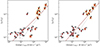 |
Fig. 1. LIR as a function of (left) global |


The fitting results of the  − LIR relations are log LIR = (0.53 ± 0.03)log
  + (7.5 ± 0.3) and log LIR = (0.61 ± 0.03)log
  + (6.9 ± 0.2), as plotted by solid lines in Fig. 1. As reference, we also plot the fitting results for single-dish measurements of the J = 3 − 2 transitions in nearby galaxies with a range of 1010 L⊙ < LIR < 1012.5 L⊙ reported by Juneau et al. (2009). Our indices (i.e., the best-fit slopes) are slightly smaller than the fitting results of Juneau et al. (2009, 0.70 ± 0.09 for HCN 3−2 and 0.81 ± 0.21 for HCO+ 3−2) and the model prediction (∼0.7 for HCN 3−2; Narayanan et al. 2008).
As an explanation for the smaller slopes in our fitting results, we note that we may systematically underestimate the line flux in the LIRGs at smaller distances. Given that the LIRG sample is chosen to have smaller distances than the ULIRG sample, the limited aperture size for spectral extraction (∼3″) and the interferometric missing flux from the extended gas components (≳3−4″) could lead to the underestimation of the line flux in the LIRG sample. The MRS of the observation of ∼3−4″ corresponds to a physical scale of ∼0.6−1.5 kpc and ∼2−3 kpc on average for LIRGs and ULIRGs, respectively. For more accurate measurements of the galaxy-integrated  , observations of a larger sample with a single-dish telescope would be essential. Alternatively, the lower gas temperature and/or the lower mean density in our LIRG sample could be responsible for the inefficient excitation of HCN and HCO+ resulting in the lower
  and
and  .
.
5. HCN/HCO+ line ratio
5.1. Global and resolved line ratio
We calculated the HCN/HCO+ line ratio ( ), based on the line luminosities extracted from the global and resolved apertures (Sect. 4.3). The results are listed in Table 4. The global
  ranges from 0.4 to 2.3 among the detected sample, with an unweighted mean of 1.1. This range is roughly comparable to that observed in the local U/LIRGs (e.g., Privon et al. 2015, for the 1−0 transitions). The resolved
  is slightly higher than the global one in most cases (16 of 20 detected cases), ranging from 0.4 to 2.7, with an unweighted mean of 1.2. This may indicate that HCN would be increased and/or more efficiently excited in the central regions compared to the galaxy average. However, we note that a high
  is also found in other parts of galaxies and is not uniquely associated with the central regions (e.g., the case of ESO 320−G030, Fig. A.22). Depending on the galaxy inclination, even the resolved
  can be a reflection of multiple velocity components along the line of sight. As detailed in Sect. 5.3, spectrally resolved analysis would be helpful to disentangle the nuclear region from the surrounding disk regions.
Measured  for the resolved and global apertures.
5.2. Comparison with galaxy properties
To consider whether  would be influenced by galaxy properties such as AGN dominance and star formation activity, we compared the global and resolved
  with mid- and far-infrared diagnostics available in the literature. As indicators of AGN dominance and strength, we used the bolometric AGN fraction (αAGN; as listed in Table 1) and the bolometric AGN luminosity (
 ; calculated as
  = αAGN Lbol, where Lbol = 1.15 LIR is assumed; Veilleux et al. 2009). We emphasize that αAGN was inferred from mid-infrared diagnostics, and this estimation should be treated with caution, particularly in the case of heavily obscured nuclei. The star formation activity was basically inferred from LIR and quantified as SFR in units of M⊙ yr−1 via the relation SFR = (1 − αAGN)×10−10LIR on the same assumption as Sturm et al. (2011), that is, the SFR–LIR relation calibrated by Kennicutt (1998) but using a Chabrier initial mass function.
In addition, we considered the possible influence by the dust temperature and the elemental N/O ratio. As a proxy of the temperature of the warm dust component, we used the IRAS 60 μm/100 μm flux density ratio (S60/S100; taken from Sanders et al. 2003). The S60/S100 color ratio of our sample ranges from 0.4 to 1.2, roughly corresponding to a dust temperature from 30 to 50 K (assuming dust emissivity proportional to (wavelength)−1; e.g., Helou et al. 1988). For the elemental N/O ratio, we used the far-infrared fine-structure line ratio of [N II]122/[O III]88 (calculated from galaxy-integrated line fluxes; taken from Díaz-Santos et al. 2017) as a rough estimator. We note that the [N II]122/[O III]88 line ratio is roughly scaled by the elemental N/O abundance ratio, but it would highly depend on the ionization parameter and the effective temperature of the ionizing source (e.g., Pereira-Santaella et al. 2017; Herrera-Camus et al. 2018). We only considered 12 galaxies in which both the [N II]122 and [O III]88 lines are detected with good significance, and hence the sample size is smaller than the parent sample in this work.
We performed a Spearman rank correlation analysis for the six above-mentioned quantities with each of the global and resolved  using pymccorrelation6 (Privon et al. 2020), which implements Monte Carlo-based methods of uncertainty estimation introduced by Curran (2014). The galaxies in which either HCN or HCO+ was not detected (i.e., UGC 11763, UGC 2982, and NGC 5734) were excluded in the analysis. The coefficients and p-values are summarized in Table 5. Correlation plots are shown in Figs. 2 and 3 for the global and resolved
  , respectively. We found no apparent correlations between
  and any of the galaxy properties.
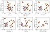 |
Fig. 2. Comparison of global |


Spearman rank coefficients and p-values.
5.2.1. Uncorrelated AGN strength
The Spearman test suggests that AGN dominance (αAGN) does not correlate with either the global  or the resolved one (Table 5). The same analysis for AGN strength itself (
 ) also showed no clear correlation with the global ratio nor the resolved one. Based on the p-values, we cannot reject the null hypothesis that the line ratio and AGN strength are uncorrelated in our sample.
Whether  correlates with AGN dominance has been a controversial issue (e.g., Graciá-Carpio et al. 2008; Privon et al. 2015; Imanishi et al. 2019). Our results are qualitatively consistent with Privon et al. (2020), for example, who found no correlation between the line ratio and X-ray measurements of AGN. The HCN enhancement by X-ray ionization from the AGN, if any, does not seem to significantly contribute to elevated
  in ≳100 pc apertures when multiple gas components with different physical and chemical conditions are laid along the line of sight.
5.2.2. Uncorrelated star formation activity
Based on the Spearman test, we found no evidence for a correlation between LIR and the global  or between LIR and the resolved one (Table 5). The result is the same as for the SFR corrected for the AGN contribution with the global ratio and with the resolved one. Although both
  and
and  themselves are correlated with LIR (Sect. 4.4),
  shows no clear trend with LIR or the SFR. The variation of
  among galaxies on ≳100 pc scales cannot be accounted for by the difference in star formation activity. This result is consistent with the findings of Tan et al. (2018) and Israel (2023), who studied samples including galaxies with lower LIR.
5.2.3. Uncorrelated dust temperature
The Spearman test showed that the S60/S100 color ratio does not correlate with the global  or the resolved one (Table 5). The large p-values suggest that
  may be unrelated to the dust temperature on ≳100 pc scales. We note that Tan et al. (2018) also found a qualitatively similar result.
5.2.4. Marginally correlated N/O abundance ratio
According to the Spearman test, the [N II]122/[O III]88 line ratio may moderately correlate with the global  (ρ =
(ρ =  , p-value =
  ), although the p-value indicates that the two quantities may be uncorrelated with a probability of ∼10%. The correlation appears less significant when tested with the resolved line ratio (ρ =
  , p-value =
  ). Considering that the [N II]122/[O III]88 line ratio is the galaxy-averaged value and both line ratios would be affected by the line optical depths, it would be reasonable that the correlation is weaker for the resolved
  .
.
The suggested possible correlation is consistent with the fact that in subsolar-metallicity dwarf galaxies,  is smaller than that of solar-metallicity galaxies (e.g., Nishimura et al. 2016a,b; Braine et al. 2017). Considering that
  can also be affected by the molecular chemistry, depending on the local physical conditions, this would imply that we should take into account the different elemental N/O abundances for the galaxies with different metallicities in order to highlight the peculiar molecular chemistry in specific regions. More accurate measurements of elemental abundances with a similar spatial resolution to molecular observations would be important for a robust and deeper understanding.
5.3. Spectrally resolved line ratio
The challenges in studying the kinematics of galaxies using molecular lines lie in limited spatial resolution and the faintness of the line emission. The situation has greatly improved with the advent of ALMA, as demonstrated by earlier studies (e.g., García-Burillo et al. 2014; Martín et al. 2015; Saito et al. 2018). These studies are, however, often restricted to individual sources and may lack sufficient spatial and/or spectral resolution to resolve the gas morphology. Our current study stands out due to its unique combination of homogeneously high sensitivity and a relatively large sample size. Leveraging this advantage, our aim is to investigate  in a spatially and spectrally resolved manner.
To explore the variation of  across different positions and different velocities within each galaxy, we generated cubes of
  and conducted analyses in both a spectrally integrated manner (pixel-by-pixel analysis) and a spectrally resolved manner (spaxel-by-spaxel analysis). Each pixel and spaxel has dimensions of 0.05″ × 0.05″ and 0.05″ × 0.05″ × 20 km s−1, respectively, for all galaxies.
For a pixel-by-pixel analysis, we initially performed spectral integration followed by applying a 3σ threshold clipping. In the spaxel-by-spaxel analysis, we first adopted a 3σ threshold clipping to both HCN and HCO+ cubes and then calculated the ratio only for the spaxels where line emission from both species is detected with a greater than 3σ significance. The adoption of the 3σ threshold clipping for the spaxels was primarily to reduce the contamination by the random Gaussian noise. We note, however, that faint but real emission contained in spaxels with a less than 3σ significance may be ignored by the clipping.
Table 6 summarizes the key statistical features, including the mean, the 25th−50th−75th and 90th percentiles, and the interquartile range for both the pixel-by-pixel and spaxel-by-spaxel analyses. Figure 4 visualizes the same quantities for 20 galaxies significantly detected in both HCN and HCO+ emission (i.e., all the sample galaxies excluding UGC 11763, UGC 2982, and NGC 5734). In general, the spectrally resolved (spaxel-by-spaxel) ratio tends to exhibit a wider range of values than the spectrally integrated (pixel-by-pixel) ratio within each galaxy. This broadening of the range is most significant and toward larger values in eight galaxies with known molecular outflows except for NGC 6240 (seven in the left-most side and one in the right-most side of Fig. 4).
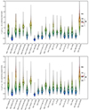 |
Fig. 4. Violin plots for |

 on a pixel-by-pixel basis and on a spaxel-by-spaxel basis.
In some galaxies, the high  regions show spatially and kinematically symmetric structures. The characteristic structure clearly emerged when we picked out the spaxels with
  higher than the 90th percentile from all spaxels in both HCN and HCO+ in each galaxy. In Figs. 5–8, we present visualization of spaxels with
  exceeding the 90th percentile in the position-position-velocity (ppV) space for 10 galaxies with known molecular out- and/or inflows (see Table 1). Indeed, symmetric morphology can be found in eight galaxies shown in Figs. 5–7. The morphology can be roughly categorized into two types: a filled bicone (IRAS 17208−0014 and IRAS 13120−5453; Fig. 5) and a thin spherical shell (IRAS 09022−3615, IRAS F14378−3651, IRAS F05189−2524, IRAS F10565+2448, IRAS 19542+1110, and ESO 320−G030; Figs. 6 and 7). For NGC 6240 and IRAS 17578−0400 (Fig. 8), the spaxels with a high line ratio appear randomly in the ppV space, likely in part because of the unsubtracted continuum in IRAS 17578−0400. For simplicity, we used the 90th percentile as a threshold for all galaxies. Through visual inspection, we found the 90th percentile generally produces suitable results to extract characteristic structures, as compared to the other neighboring values such as the 85th and 95th percentile. Understanding the underlying physics that make this threshold effective could be an interesting theme for future studies.
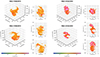 |
Fig. 5. Visualizations of |

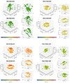 |
Fig. 6. Same as Fig. 5 but for IRAS 09022−3615, IRAS F14378−3651, IRAS F05189−2524, and IRAS F10565+2448. |
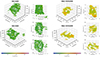 |
Fig. 8. Same as Fig. 5 but for NGC 6240 and IRAS 17578−0400. We note that the continuum has not been subtracted for IRAS 17578−0400. |
For reference, the ppV plots for the entire set of spaxels as well as for those spaxels that exceed the 90th percentile within individual galaxies for all galaxies in our sample are presented in Appendix B. We note that the symmetry is rather distorted, but it is marginally seen in ESO 148−IG002 and ESO 173−G015. In the other galaxies, such symmetry is not noticeable, as we discuss in Appendix C.
5.4. Relation to outflows and inflows
As mentioned in the previous section, symmetric structures of high  are present in some of our sample (Figs. 5–7). Notably, such symmetric structures are predominantly found in galaxies with molecular outflows and/or inflows previously found by CO and/or OH line observations. For a descriptive comparison with key parameters of out- and inflows found in the literature, we encourage readers to refer to Appendix C. If we consider that the high
  regions are associated with the gas shocked by the out- and/or inflowing materials, plotting
  in the ppV space could be a useful method to look for out- and inflows and study their geometry independently from kinematic modeling.
In our sample, symmetrically enhanced HCN is frequently seen in ULIRGs and is rare in LIRGs. Our results may suggest that nuclear feeding and feedback are predominantly taking place in IR-brighter galaxies. However, fast shocks (vshock ≳ 20 km s−1) may be required for the prominent enhancement of HCN (see Sect. 6.2 for details), and thus we cannot rule out the presence of out- and inflows with slower shocks or no shock in our sample galaxies.
6. Discussion
As presented in Figs. 4 and B.1,  varies greatly from galaxy to galaxy and from position to position within each galaxy. In a galaxy-to-galaxy comparison,
  shows no clear correlation with galaxy properties such as AGN dominance, but it might be marginally scaled by the elemental N/O ratio (Sect. 5.2). On the other hand, the variation of
  in the ppV space of each galaxy seems to be related to out- and inflows. In this section, we try to figure out the most critical factor for the elevation of
  in out- and inflows. We discuss
  with regard to molecular abundances and excitation conditions, by non-LTE radiative transfer calculations (Sect. 6.1). We also consider the excitation by collision with electrons, which could be effective for HCN in a moderately dense condition (Goldsmith & Kauffmann 2017). With constraints on the molecular abundances obtained from the non-LTE analysis, we ran chemical models and tested if shocks can reproduce the line ratio observed in out- and inflows (Sect. 6.2).
6.1. Excitation conditions
To inspect the molecular abundances and excitation conditions for the observed  , we made calculations to study the line ratios as functions of gas density in various physical conditions. Given that both HCN and HCO+ are likely to be subthermally excited (see Sect. 4.4), we adopted the non-local thermal equilibrium (non-LTE) radiative transfer model, assuming uniform sphere geometry with a large velocity gradient (LVG, see e.g., Goldreich & Kwan 1974). Practically, we used a publicly available code, RADEX7 (van der Tak et al. 2007), to predict the line intensity. RADEX requires five input parameters: the background temperature, the column density of the molecular species in question, the line width, the kinetic temperature, and the H2 density. In all of our calculations, the background temperature was fixed to be the temperature of the cosmic microwave background (i.e., 2.7 K). We note that the background temperature could be higher in the nuclear region, but this fixed temperature assumption is acceptable for a large part of each outflow when considering that the continuum emission is much more compact (e.g., Pereira-Santaella et al. 2021). We implemented the molecular column density as a product of the H2 column density (NH2) and a fractional abundance of the species (Xmol). For NH2, we considered three plausible values for U/LIRGs: 1022, 1023, and 1024 cm−2. We varied XHCN to cover a wide range of values: 1 × 10⁻⁸, 5 × 10⁻⁸, 1 × 10⁻⁷, 3 × 10⁻⁷, and 5 × 10⁻⁷. On the other hand, XHCO+ was fixed to the reference value 10−8. The validity of these fractional abundances are discussed in Sect. 6.2. The line width (Δv) was set to be 50 km s−1. This value is somewhat smaller than the observed values, but we can consider the emission as arising from an ensemble of such clouds. We explored three values for the kinetic temperature (Tkin): 20, 50, and 100 K. The H2 density (nH2) was set to 100 values logarithmically spaced in a range from 101 cm−3 to 109 cm−3. The collisional rate coefficients are taken from Dumouchel et al. (2010) for HCN and from Denis-Alpizar et al. (2020) for HCO+.
As partners for collisional excitation, we additionally took into account free electrons. This was motivated by the indication from Goldsmith & Kauffmann (2017) that electron excitation can be more significant for HCN compared to HCO+ when the electron fractional abundance is ≳10−5 and the gas density is ≲105.5 cm−2 (Goldsmith & Kauffmann 2017). In addition to the case without collision with electrons, we explored cases with fractional abundances of electrons (Xe−) of 10−5 and 10−4, which could be achieved if the cosmic-ray ionization rate is high (ζ ≳ 10−15 s−1), such as in the vicinity of supernova remnants (Ceccarelli et al. 2011). This type of high cosmic-ray ionization rate is indeed reported for the nearby starburst galaxy NGC 253 (Harada et al. 2021; Holdship et al. 2022). We note that the electron abundance was implemented into RADEX calculations in the form of a volume density of electrons (ne− = nH2Xe−). The collisional rate coefficients for the HCN are taken from Faure et al. (2007). For HCO+, the published collisional rate coefficients are only available for J ≤ 3 levels (Faure & Tennyson 2001; Singh 2021). As pointed out by Goldsmith & Kauffmann (2017), these rate coefficients are comparable to those of HCN and consistent with scaling with the square of the dipole moment (μ2). We provisionally employed the rate coefficients for J ≥ 3 levels generated by scaling with μ2 based on the rate coefficients for HCN provided by Faure et al. (2007). For a robust discussion in the future, more accurate rate coefficients for HCO+ will be necessary.
We ran RADEX with all combinations of parameters described above and calculated  as a function of nH2. The results are plotted in Fig. 9. Each of the nine panels correspond to a different pairing of NH2 and Tkin. The different colors and line styles in the figure are employed to represent the varying values of XHCN, XHCO+, and Xe−. Consistent with such studies as Butterworth et al. (2022) and Imanishi et al. (2023), Fig. 9 indicates that
  increases as XHCN/XHCO+ increases for any pairings of NH2 and Tkin. As also noted in Yamada et al. (2007) and Izumi et al. (2016), for example, XHCN/XHCO+ ≳ 10 is necessary to get
  ≳ 1 unless the density is very high (≳106 cm−3).
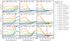 |
Fig. 9. One-zone non-LTE calculation of |


The H2 density also plays an important role in regulating  . In the cases with low NH2 (left panels in Fig. 9),
  becomes larger at higher densities. This is because HCO+ emission is brightest at densities slightly above its effective critical H2 density and is a bit less bright at the highest densities, while HCN emission behaves similarly but with a larger intensity at a higher density. This trend is less pronounced as NH2 increases because HCN and HCO+ emission becomes similarly bright when they are thermalized at high density. In cases with XHCN > 10−7, bumps of
  are seen in the density range of 102 − 105 cm−3. These bumps are attributed to the different effective critical density between HCN and HCO+ (for reference: 2.5 × 104 cm−3 for NHCN = 1014 cm−2 and 2.6 × 103 cm−3 for NHCO+ = 1014 cm−2, both for Tkin = 50 K; Shirley 2015). Because of radiative trapping, the effective critical density is roughly scaled by the inverse of Nmol. As NHCN increases, the effective critical density of HCN decreases, and hence the bump tends to appear at a lower density and becomes more pronounced. With XHCN/XHCO+ = 10 (green curves in Fig. 9), which results in
  of ∼1, the effective critical densities of HCN and HCO+ become quite similar, and thus the
  curves are almost flat around the critical density. We also tested different reference abundances of HCO+, such as XHCO+ = 10−7, and found qualitatively similar trends.
Another notable feature is that a contribution from electron excitation significantly increases  at moderate H2 densities (∼103 − 105 cm−3). The effect is especially noticeable when the electron abundance is highest (Xe− = 10−4) and the HCN abundance is also high (XHCN > 1 × 10⁻⁷), in which case
  can be more than twice as much as the ratio without electron excitation.
In the case with NH2 = 1024 cm−2 and Tkin = 50 and 100 K (lower two panels on the right side of Fig. 9), there are spikes at nH2 ∼ 105 − 107 cm−3, which are caused by population inversion between the J = 2 and 3 levels of HCN. Because these variations are only seen for a very limited range of parameters, we consider the influence of such population inversion to be negligible in most observations.
In summary, our one-zone models indicate that  can attain high values (> 1) when X(HCN)/X(HCO+) exceeds 10 for a significant range of densities.
  will be further enhanced if electron abundance is considerably high (Xe− = 10−4).
6.2. Chemical pathways to the enhancement of HCN
Formation and destruction processes of molecules can be influenced by physical conditions. Galactic outflows and inflows can be distinguished from other parts of the galaxy by chemistry induced by shocks. Shock heating affects both gas-phase and grain-surface reactions and releases species in the icy grain mantles into the gas phase (e.g., Bachiller et al. 2001). Non-thermal desorption, such as sputtering, also helps in mantle release (e.g., Bachiller et al. 2001). In addition, outflows can induce turbulence at the interface between molecular clouds, enabling a continuous exposure of the gas to X-ray, UV, and/or cosmic-ray radiation at the surface. This process can lead to an effective ionization and, in turn, a refreshment of the molecular composition (García-Burillo et al. 2017).
The enhancement of HCN abundances in shocked regions is well known for protostellar outflows (e.g., L1157; Bachiller & Pérez Gutiérrez 1997), and many chemical models have been developed to reproduce the observed abundances (e.g., Burkhardt et al. 2019). Those chemical models consider the physical conditions as representative of protostellar outflows: the gas density is set to be as high as ∼105 cm−3. Under such density conditions, HCN abundances in the gas phase are enhanced immediately after the passage of shocks (post-shock time of < 102 yr) up to XHCN ∼ 10−5 due to the release of the ice population by grain heating and sputtering (see e.g. Fig. 4 of Burkhardt et al. 2019). This enhancement mechanism of HCN could be applied to the case of galactic outflows and could be able to account, at least in part, for the observed line ratios in our sample. However, given that the majority of the gas is in a density range of ∼103 − 104 cm−3 in the beam of extragalactic observations, it is essential to consider the chemistry in the moderately-dense regime.
To examine how shocks affect the chemistry in the moderately-dense gas (∼103 − 104 cm−3), we experimentally ran the time-dependent gas-grain chemical code, UCLCHEM8 (Holdship et al. 2017), which is publicly available. We adopted the “C-shock” model of UCLCHEM, which is based on the parameterization of C-type shocks by Jiménez-Serra et al. (2008). For details, we refer to Viti et al. (2014), García-Burillo et al. (2017), and Holdship et al. (2017), where models similar to ours were computed. Here, we provide a concise overview of the most critical aspects. The model was run in two phases: the pre-shock and post-shock phases. As a pre-shock condition, we considered the typical condition of “standard” molecular gas with Galactic elemental abundances. The pre-shock abundances follow the method employed by Harada et al. (2019): all physical conditions were kept constant at standard Galactic values (H2 density 103 cm−3, temperature 10 K, visual extinction 2 mag, radiation field 1 Habing, cosmic ionization rate 1.3 × 10⁻¹⁷ s−1; we note that these values are provisional and should be better calibrated for U/LIRGs in future works). The evolution of the molecular abundances in the gas phase and on the grain surfaces were calculated as a function of time using rate equations. The chemical evolution was followed for 105 yr in the pre-shock phase to reproduce realistic molecular abundances observed on cloud scales (> 10 pc; Harada et al. 2019). In the post-shock phase, we tested four values of shock velocity: 10, 20, 30, and 40 km s−1. During this phase, the density, temperature, and velocity profile were varied as a function of time, following the parameterizations of the shock model. Our model maintained constant values for the radiation field and the cosmic-ray ionization rate, but it is worth noting that these parameters would also fluctuate in a real molecular cloud.
In Fig. 10, the evolution of the gas temperature and density as well as the abundances of HCN, HCO+, and the electrons are shown as a function of post-shock time. As shown in Fig. 10, the HCN abundance is enhanced by a factor of ∼10−100 at ∼103 − 105 yr after the shock, depending on the shock velocity. On the other hand, the HCO+ and electron abundances are decreased during the HCN enhancement. It appears that the HCN abundance falls back to the pre-shock abundance at a post-shock time of ∼105 yr. This timescale is roughly comparable to the dynamical time of outflows (calculated as Rout/vout).
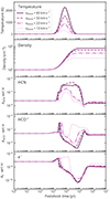 |
Fig. 10. Chemical model predictions to simulate gas temperature, density, and fractional abundances of HCN, HCO+, and electrons under moderately-dense conditions (nH2 ∼ 103 − 104 cm−3). C-type shocks with shock velocities of 10, 20, 30, and 40 km s−1 are considered. The pre-shock H2 density is assumed to be 103 cm−2 for all cases. More details on the other assumed parameters are described in Sect. 6.2. |
In our model, unlike the chemistry under the high density conditions, thermal desorption or sputtering do not contribute to the HCN enhancement because HCN ice is almost absent in pre-shock conditions. Instead, the enhancement of HCN is mainly due to the gas-phase production via the high-temperature reaction: CN + H2 → HCN + H. Because the rate coefficient of this reaction is a function of temperature (k = α(T/300 K)βexp(−γ/T) where α = 4 × 10⁻¹³, β = 2.87, γ = 820 K, and T is temperature; Harada et al. 2010), the degree of HCN enhancement depends on the heating. Consequently, the shock velocity affects the degree of HCN enhancement. As shown in Fig. 10, shock velocities of 30 and 40 km s−1 can reproduce our HCN and HCO+ abundances, accounting for the observed line ratio, while 10 and 20 km s−1 shocks seem to be insufficient. As mentioned in Appendix C, the HCN enhancement was not found in NGC 6240, and it might be because the shock velocity is too small to enhance the HCN abundance (Meijerink et al. 2013). However, considering the results of a high-resolution study in the CO J = 2 − 1 line, which highlighted the existence of very high-velocity outflows (Saito et al. 2018), NGC 6240 deserves further investigation.
The key reaction (CN + H2 → HCN + H) suggests that HCN abundance increases at the expense of CN abundance. Considering that Mrk 231 has an outflow that is notably bright in both CN (Cicone et al. 2020) and HCN (Aalto et al. 2015b; Lindberg et al. 2016), it is likely that CN abundance is maintained by the high ionization rate in the outflow. In environments where C+ is abundant, CN can be rapidly formed. A similar rationale can be applied to the CCH-bright outflow in NGC 1068, as discussed in García-Burillo et al. (2017). We also note that CN emission is less affected by electron excitation than HCN (Goldsmith & Kauffmann 2017). This would provide an additional support for the enhancement of HCN abundance in outflows.
7. Summary and conclusions
We conducted observations of the HCN and HCO+J = 3 − 2 lines toward 23 U/LIRGs in the local Universe (z < 0.07). The spatial resolution was ∼0.3″, which corresponds to ∼50−400 pc at the distance of each target. The obtained dataset allowed us to explore the HCN/HCO+ line ratio ( ) of each galaxy in a spatially and spectrally resolved manner. We analyzed
  in relation to the galaxy properties such as AGN dominance and star formation activity, and we found the presence of outflows and/or inflows to have the most crucial influence. Non-LTE radiative transfer analysis and chemical models suggest that a higher HCN abundance in shocked regions is likely to be responsible for a high
  in out- and inflows.
The main results and key points from the analysis are the following:
-
Spectra and moment maps. The line emission of HCN and HCO+ was successfully detected with a signal-to-noise ratio of > 5σ in 21 out of the 23 galaxies. The line profiles of HCN and HCO+ are often complex and cannot be fitted by a single Gaussian. The HCN and HCO+ emission is mostly emitted from a central region of each galaxy. The apparent size of the line-emitting region is typically 1−3 kpc in ULIRGs and 0.5−1 kpc in LIRGs. In almost all the galaxies with known molecular outflows, the velocity dispersion of the HCN emission is higher than that of HCO+.
-
Correlation between line luminosity and infrared luminosity. We found
 and
and  correlate well with LIR (correlation coefficients of 0.85 and 0.90, respectively). These relations are quantitatively consistent with previous observations and model predictions. The
  –LIR and
  –LIR slopes of ∼0.5−0.6 suggest that HCN and HCO+ are ubiquitously distributed in the molecular gas with a wide range of densities, and most of them are subthermally excited.
 -
Line ratio and its correlation with galaxy properties. The velocity-integrated
 extracted from a large aperture (∼3″) in each galaxy is in the range of 0.4−2.3. The unweighted mean is 1.1. Although the HCN/HCO+ has been proposed as AGN/starburst diagnostics in the literature, we found no evidence for correlations of
  with AGN dominance, star formation activity, or dust temperature. The elemental N/O ratio potentially moderately correlates with
  , although p-values suggest that those quantities may be uncorrelated, with a probability of ∼10%.
 -
Spatially and spectrally resolved line ratios. We explored the variation of
 in the ppV space of each galaxy. As a result,
  considerably varies from spaxel to spaxel, even within a galaxy. We found spatially and kinematically symmetric structures of high line ratio (the highest 10th percentile on a spaxel-by-spaxel basis) in some galaxies. Such structures are predominantly found in galaxies with molecular outflows previously found by CO and/or OH line observations.
 -
Non-LTE radiative transfer analysis. One-zone non-LTE radiative transfer calculations were made to investigate the excitation conditions and molecular abundances in the gas phase in our sample galaxies. They revealed that
 depends on many parameters, such as the HCN/HCO+ abundance ratio, H2 volume density, and electron abundances. Taking all factors into consideration, the observed high
  (> 1) in outflows and inflows are essentially caused by a high HCN/HCO+ abundance ratio, and this can be further enhanced by electrons.
 -
Key chemical process to enhance HCN abundance. Chemistry induced by shocks characterizes the molecular abundances in outflows and inflows. As reported by previous studies, thermal and non-thermal release of HCN ice mostly contributes to the enhancement of HCN in the gas phase under high density conditions (∼105 cm−3). In the moderately-dense gas, which accounts for a larger fraction of the total gas, the HCN abundance is mainly enhanced by a high-temperature gas-phase reaction: CN + H2 → HCN + H. The post-shock time of HCN enhancement is roughly comparable to the dynamical time of the outflow (∼105 yr).
Finally, we emphasize the advantages of analyzing  in a spatially and spectrally resolved manner. Considering that the mass of the regions influenced by outflows and/or inflows is smaller than the total mass of the galaxy, spatial or spectral integration may make it difficult to distinguish shocked regions from others. Our results imply that the spatially and spectrally resolved
  helps identify the geometry of outflows and inflows, at least in some cases, when the shock velocity of the outflows is sufficiently high to heat the gas. To develop line diagnostics for the characterization of physical properties of U/LIRGs, further exploration of molecular compositions and more detailed modeling of the kinematic structure of a galaxy should be investigated in future studies.
Throughout this paper, “line ratio” refers to the line intensity ratio or, equivalently, the line luminosity ratio. The line luminosity L′ is expressed in units of K km s−1 pc2.
Acknowledgments
We thank the anonymous referee for a constructive report that significantly contributed to the improvement of this paper. We thank Niklas Falstad for valuable discussions and for the earlier work on CON-quest. Y.N. gratefully acknowledges support by JSPS KAKENHI grant No. JP23K13140, JP18K13577, and NAOJ ALMA Scientific Research Grant No. 2017-06B. S.A. and S.K. gratefully acknowledge funding from the European Research Council (ERC) under the European Union’s Horizon 2020 research and innovation programme (grant agreement No. 789410). S.A. and M.G. also acknowledge support from Swedish Research Council grant 621-2011-4143. J.S.G. thanks the University of Wisconsin College of Letters and Science for partial support of this research. E.G.-A. thanks the Spanish MICINN for support under projects PID2019-105552RB-C41 and PID2022-137779OB-C41. K.K. acknowledges the support by JSPS KAKENHI Grant Number JP17H06130 and the NAOJ ALMA Scientific Research Grant No. 2017-06B. M.I. is supported by JSPS KAKENHI grant No. JP21K03632. C.R. acknowledges support from Fondecyt Regular grant 1230345 and ANID BASAL project FB210003. This paper makes use of the following ALMA data: ADS/JAO.ALMA#2017.1.00759.S and ADS/JAO.ALMA#2018.1.01344.S. ALMA is a partnership of ESO (representing its member states), NSF (USA) and NINS (Japan), together with NRC (Canada), MOST and ASIAA (Taiwan), and KASI (Republic of Korea), in cooperation with the Republic of Chile. The Joint ALMA Observatory is operated by ESO, AUI/NRAO and NAOJ. S.A. and M.G. also acknowledge support from Swedish Research Council grant 621-2011-4143
References
- Aalto, S., Spaans, M., Wiedner, M. C., & Hüttemeister, S. 2007, A&A, 464, 193 [NASA ADS] [CrossRef] [EDP Sciences] [Google Scholar]
- Aalto, S., Martín, S., Costagliola, F., et al. 2015a, A&A, 584, A42 [NASA ADS] [CrossRef] [EDP Sciences] [Google Scholar]
- Aalto, S., Garcia-Burillo, S., Muller, S., et al. 2015b, A&A, 574, A85 [NASA ADS] [CrossRef] [EDP Sciences] [Google Scholar]
- Aalto, S., Muller, S., König, S., et al. 2019, A&A, 627, A147 [NASA ADS] [CrossRef] [EDP Sciences] [Google Scholar]
- Astropy Collaboration (Robitaille, T. P., et al.) 2013, A&A, 558, A33 [NASA ADS] [CrossRef] [EDP Sciences] [Google Scholar]
- Astropy Collaboration (Price-Whelan, A. M., et al.) 2018, AJ, 156, 123 [Google Scholar]
- Bachiller, R., & Pérez Gutiérrez, M. 1997, ApJ, 487, L93 [Google Scholar]
- Bachiller, R., Pérez Gutiérrez, M., Kumar, M. S. N., & Tafalla, M. 2001, A&A, 372, 899 [NASA ADS] [CrossRef] [EDP Sciences] [Google Scholar]
- Barcos-Muñoz, L., Aalto, S., Thompson, T. A., et al. 2018, ApJ, 853, L28 [Google Scholar]
- Bayet, E., Viti, S., Williams, D. A., & Rawlings, J. M. C. 2008, ApJ, 676, 978 [NASA ADS] [CrossRef] [Google Scholar]
- Braine, J., Shimajiri, Y., André, P., et al. 2017, A&A, 597, A44 [NASA ADS] [CrossRef] [EDP Sciences] [Google Scholar]
- Burkhardt, A. M., Shingledecker, C. N., Le Gal, R., et al. 2019, ApJ, 881, 32 [Google Scholar]
- Bussmann, R. S., Narayanan, D., Shirley, Y. L., et al. 2008, ApJ, 681, L73 [NASA ADS] [CrossRef] [Google Scholar]
- Butterworth, J., Holdship, J., Viti, S., & García-Burillo, S. 2022, A&A, 667, A131 [NASA ADS] [CrossRef] [EDP Sciences] [Google Scholar]
- CASA Team (Bean, B., et al.) 2022, PASP, 134, 114501 [NASA ADS] [CrossRef] [Google Scholar]
- Ceccarelli, C., Hily-Blant, P., Montmerle, T., et al. 2011, ApJ, 740, L4 [NASA ADS] [CrossRef] [Google Scholar]
- Cicone, C., Maiolino, R., Sturm, E., et al. 2014, A&A, 562, A21 [NASA ADS] [CrossRef] [EDP Sciences] [Google Scholar]
- Cicone, C., Severgnini, P., Papadopoulos, P. P., et al. 2018, ApJ, 863, 143 [NASA ADS] [CrossRef] [Google Scholar]
- Cicone, C., Maiolino, R., Aalto, S., Muller, S., & Feruglio, C. 2020, A&A, 633, A163 [NASA ADS] [CrossRef] [EDP Sciences] [Google Scholar]
- Costagliola, F., Aalto, S., Rodriguez, M. I., et al. 2011, A&A, 528, A30 [NASA ADS] [CrossRef] [EDP Sciences] [Google Scholar]
- Costagliola, F., Aalto, S., Sakamoto, K., et al. 2013, A&A, 556, A66 [NASA ADS] [CrossRef] [EDP Sciences] [Google Scholar]
- Curran, P. A. 2014, arXiv e-prints [arXiv:1411.3816] [Google Scholar]
- Denis-Alpizar, O., Stoecklin, T., Dutrey, A., & Guilloteau, S. 2020, MNRAS, 497, 4276 [Google Scholar]
- Díaz-Santos, T., Armus, L., Charmandaris, V., et al. 2017, ApJ, 846, 32 [Google Scholar]
- Dumouchel, F., Faure, A., & Lique, F. 2010, MNRAS, 406, 2488 [NASA ADS] [CrossRef] [Google Scholar]
- Falstad, N., Hallqvist, F., Aalto, S., et al. 2019, A&A, 623, A29 [NASA ADS] [CrossRef] [EDP Sciences] [Google Scholar]
- Falstad, N., Aalto, S., König, S., et al. 2021, A&A, 649, A105 [NASA ADS] [CrossRef] [EDP Sciences] [Google Scholar]
- Faure, A., & Tennyson, J. 2001, MNRAS, 325, 443 [NASA ADS] [CrossRef] [Google Scholar]
- Faure, A., Varambhia, H. N., Stoecklin, T., & Tennyson, J. 2007, MNRAS, 382, 840 [Google Scholar]
- Fluetsch, A., Maiolino, R., Carniani, S., et al. 2019, MNRAS, 483, 4586 [NASA ADS] [Google Scholar]
- Gao, Y., & Solomon, P. M. 2004, ApJS, 152, 63 [Google Scholar]
- García-Burillo, S., Combes, F., Usero, A., et al. 2014, A&A, 567, A125 [Google Scholar]
- García-Burillo, S., Combes, F., Usero, A., et al. 2015, A&A, 580, A35 [Google Scholar]
- García-Burillo, S., Viti, S., Combes, F., et al. 2017, A&A, 608, A56 [Google Scholar]
- Goldreich, P., & Kwan, J. 1974, ApJ, 189, 441 [CrossRef] [Google Scholar]
- Goldsmith, P. F., & Kauffmann, J. 2017, ApJ, 841, 25 [Google Scholar]
- González-Alfonso, E., Fischer, J., Spoon, H. W. W., et al. 2017, ApJ, 836, 11 [Google Scholar]
- González-Alfonso, E., Pereira-Santaella, M., Fischer, J., et al. 2021, A&A, 645, A49 [EDP Sciences] [Google Scholar]
- Gorski, M. D., Aalto, S., König, S., et al. 2023, A&A, 670, A70 [NASA ADS] [CrossRef] [EDP Sciences] [Google Scholar]
- Graciá-Carpio, J., García-Burillo, S., Planesas, P., Fuente, A., & Usero, A. 2008, A&A, 479, 703 [NASA ADS] [CrossRef] [EDP Sciences] [Google Scholar]
- Hagiwara, Y., Baan, W. A., & Klöckner, H.-R. 2011, AJ, 142, 17 [NASA ADS] [CrossRef] [Google Scholar]
- Harada, N., Herbst, E., & Wakelam, V. 2010, ApJ, 721, 1570 [NASA ADS] [CrossRef] [Google Scholar]
- Harada, N., Thompson, T. A., & Herbst, E. 2013, ApJ, 765, 108 [NASA ADS] [CrossRef] [Google Scholar]
- Harada, N., Sakamoto, K., Martín, S., et al. 2018, ApJ, 855, 49 [Google Scholar]
- Harada, N., Nishimura, Y., Watanabe, Y., et al. 2019, ApJ, 871, 238 [NASA ADS] [CrossRef] [Google Scholar]
- Harada, N., Martín, S., Mangum, J. G., et al. 2021, ApJ, 923, 24 [NASA ADS] [CrossRef] [Google Scholar]
- Helou, G., Khan, I. R., Malek, L., & Boehmer, L. 1988, ApJS, 68, 151 [NASA ADS] [CrossRef] [Google Scholar]
- Herrera-Camus, R., Sturm, E., Graciá-Carpio, J., et al. 2018, ApJ, 861, 94 [Google Scholar]
- Holdship, J., Viti, S., Jiménez-Serra, I., Makrymallis, A., & Priestley, F. 2017, AJ, 154, 38 [NASA ADS] [CrossRef] [Google Scholar]
- Holdship, J., Mangum, J. G., Viti, S., et al. 2022, ApJ, 931, 89 [NASA ADS] [CrossRef] [Google Scholar]
- Hopkins, P. F., Somerville, R. S., Hernquist, L., et al. 2006, ApJ, 652, 864 [NASA ADS] [CrossRef] [Google Scholar]
- Imanishi, M., & Nakanishi, K. 2013, AJ, 146, 91 [Google Scholar]
- Imanishi, M., Nakanishi, K., Tamura, Y., & Peng, C.-H. 2009, AJ, 137, 3581 [Google Scholar]
- Imanishi, M., Nakanishi, K., & Izumi, T. 2019, ApJS, 241, 19 [Google Scholar]
- Imanishi, M., Baba, S., Nakanishi, K., & Izumi, T. 2023, ApJ, 950, 75 [NASA ADS] [CrossRef] [Google Scholar]
- Israel, F. P. 2023, A&A, 671, A59 [NASA ADS] [CrossRef] [EDP Sciences] [Google Scholar]
- Izumi, T., Kohno, K., Aalto, S., et al. 2016, ApJ, 818, 42 [NASA ADS] [CrossRef] [Google Scholar]
- Jiménez-Donaire, M. J., Bigiel, F., Leroy, A. K., et al. 2019, ApJ, 880, 127 [CrossRef] [Google Scholar]
- Jiménez-Serra, I., Caselli, P., Martín-Pintado, J., & Hartquist, T. W. 2008, A&A, 482, 549 [NASA ADS] [CrossRef] [EDP Sciences] [Google Scholar]
- Juneau, S., Narayanan, D. T., Moustakas, J., et al. 2009, ApJ, 707, 1217 [NASA ADS] [CrossRef] [Google Scholar]
- Kauffmann, J., Goldsmith, P. F., Melnick, G., et al. 2017, A&A, 605, L5 [NASA ADS] [CrossRef] [EDP Sciences] [Google Scholar]
- Kawana, Y., Saito, T., Okumura, S. K., et al. 2022, ApJ, 929, 100 [NASA ADS] [CrossRef] [Google Scholar]
- Kennicutt, R. C., Jr. 1998, ApJ, 498, 541 [Google Scholar]
- Kohno, K., Matsushita, S., Vila-Vilaró, B., et al. 2001, in The Central Kiloparsec of Starbursts and AGN: The La Palma Connection, eds. J. H. Knapen, J. E. Beckman, I. Shlosman, & T. J. Mahoney, ASP Conf. Ser., 249, 672 [NASA ADS] [Google Scholar]
- Komossa, S., Burwitz, V., Hasinger, G., et al. 2003, ApJ, 582, L15 [NASA ADS] [CrossRef] [Google Scholar]
- König, S., Aalto, S., Muller, S., et al. 2018, A&A, 615, A122 [NASA ADS] [CrossRef] [EDP Sciences] [Google Scholar]
- Krips, M., Neri, R., García-Burillo, S., et al. 2008, ApJ, 677, 262 [NASA ADS] [CrossRef] [Google Scholar]
- Krumholz, M. R., & Thompson, T. A. 2007, ApJ, 669, 289 [NASA ADS] [CrossRef] [Google Scholar]
- Laurent, O., Mirabel, I. F., Charmandaris, V., et al. 2000, A&A, 359, 887 [NASA ADS] [Google Scholar]
- Lepp, S., & Dalgarno, A. 1996, A&A, 306, L21 [NASA ADS] [Google Scholar]
- Lindberg, J. E., Aalto, S., Muller, S., et al. 2016, A&A, 587, A15 [NASA ADS] [CrossRef] [EDP Sciences] [Google Scholar]
- Lutz, D., Genzel, R., Sternberg, A., et al. 1996, A&A, 315, L137 [NASA ADS] [Google Scholar]
- Lutz, D., Sturm, E., Janssen, A., et al. 2020, A&A, 633, A134 [NASA ADS] [CrossRef] [EDP Sciences] [Google Scholar]
- Maloney, P. R., Hollenbach, D. J., & Tielens, A. G. G. M. 1996, ApJ, 466, 561 [Google Scholar]
- Martín, S., Kohno, K., Izumi, T., et al. 2015, A&A, 573, A116 [NASA ADS] [CrossRef] [EDP Sciences] [Google Scholar]
- Martín, S., Aalto, S., Sakamoto, K., et al. 2016, A&A, 590, A25 [NASA ADS] [CrossRef] [EDP Sciences] [Google Scholar]
- Meijerink, R., & Spaans, M. 2005, A&A, 436, 397 [CrossRef] [EDP Sciences] [Google Scholar]
- Meijerink, R., Spaans, M., & Israel, F. P. 2007, A&A, 461, 793 [NASA ADS] [CrossRef] [EDP Sciences] [Google Scholar]
- Meijerink, R., Kristensen, L. E., Weiß, A., et al. 2013, ApJ, 762, L16 [Google Scholar]
- Montoya Arroyave, I., Cicone, C., Makroleivaditi, E., et al. 2023, A&A, 673, A13 [NASA ADS] [CrossRef] [EDP Sciences] [Google Scholar]
- Narayanan, D., Cox, T. J., Shirley, Y., et al. 2008, ApJ, 684, 996 [NASA ADS] [CrossRef] [Google Scholar]
- Nishimura, Y., Shimonishi, T., Watanabe, Y., et al. 2016a, ApJ, 829, 94 [NASA ADS] [CrossRef] [Google Scholar]
- Nishimura, Y., Shimonishi, T., Watanabe, Y., et al. 2016b, ApJ, 818, 161 [NASA ADS] [CrossRef] [Google Scholar]
- Nishimura, Y., Watanabe, Y., Harada, N., et al. 2017, ApJ, 848, 17 [NASA ADS] [CrossRef] [Google Scholar]
- Oteo, I., Zhang, Z. Y., Yang, C., et al. 2017, ApJ, 850, 170 [NASA ADS] [CrossRef] [Google Scholar]
- Pereira-Santaella, M., Colina, L., García-Burillo, S., et al. 2016, A&A, 594, A81 [NASA ADS] [CrossRef] [EDP Sciences] [Google Scholar]
- Pereira-Santaella, M., Rigopoulou, D., Farrah, D., Lebouteiller, V., & Li, J. 2017, MNRAS, 470, 1218 [NASA ADS] [CrossRef] [Google Scholar]
- Pereira-Santaella, M., Colina, L., García-Burillo, S., et al. 2021, A&A, 651, A42 [NASA ADS] [CrossRef] [EDP Sciences] [Google Scholar]
- Pérez-Torres, M., Mattila, S., Alonso-Herrero, A., Aalto, S., & Efstathiou, A. 2021, A&ARv, 29, 2 [CrossRef] [Google Scholar]
- Pety, J., Guzmán, V. V., Orkisz, J. H., et al. 2017, A&A, 599, A98 [NASA ADS] [CrossRef] [EDP Sciences] [Google Scholar]
- Privon, G. C., Herrero-Illana, R., Evans, A. S., et al. 2015, ApJ, 814, 39 [CrossRef] [Google Scholar]
- Privon, G. C., Aalto, S., Falstad, N., et al. 2017, ApJ, 835, 213 [NASA ADS] [CrossRef] [Google Scholar]
- Privon, G. C., Ricci, C., Aalto, S., et al. 2020, ApJ, 893, 149 [NASA ADS] [CrossRef] [Google Scholar]
- Ricci, C., Privon, G. C., Pfeifle, R. W., et al. 2021, MNRAS, 506, 5935 [NASA ADS] [CrossRef] [Google Scholar]
- Romano, M., Cassata, P., Morselli, L., et al. 2021, A&A, 653, A111 [NASA ADS] [CrossRef] [EDP Sciences] [Google Scholar]
- Saito, T., Iono, D., Ueda, J., et al. 2018, MNRAS, 475, L52 [NASA ADS] [CrossRef] [Google Scholar]
- Sakamoto, K., Aalto, S., Evans, A. S., Wiedner, M. C., & Wilner, D. J. 2010, ApJ, 725, L228 [Google Scholar]
- Sakamoto, K., Aalto, S., Costagliola, F., et al. 2013, ApJ, 764, 42 [Google Scholar]
- Sanders, D. B., & Mirabel, I. F. 1996, ARA&A, 34, 749 [Google Scholar]
- Sanders, D. B., Soifer, B. T., Elias, J. H., et al. 1988, ApJ, 325, 74 [Google Scholar]
- Sanders, D. B., Phinney, E. S., Neugebauer, G., Soifer, B. T., & Matthews, K. 1989, ApJ, 347, 29 [NASA ADS] [CrossRef] [Google Scholar]
- Sanders, D. B., Mazzarella, J. M., Kim, D. C., Surace, J. A., & Soifer, B. T. 2003, AJ, 126, 1607 [Google Scholar]
- Schmidt, M. 1959, ApJ, 129, 243 [NASA ADS] [CrossRef] [Google Scholar]
- Shirley, Y. L. 2015, PASP, 127, 299 [Google Scholar]
- Singh, J. 2021, MNRAS, 504, 1531 [NASA ADS] [CrossRef] [Google Scholar]
- Solomon, P. M., & Vanden Bout, P. A. 2005, ARA&A, 43, 677 [NASA ADS] [CrossRef] [Google Scholar]
- Stierwalt, S., Armus, L., Surace, J. A., et al. 2013, ApJS, 206, 1 [Google Scholar]
- Sturm, E., González-Alfonso, E., Veilleux, S., et al. 2011, ApJ, 733, L16 [NASA ADS] [CrossRef] [Google Scholar]
- Tan, Q.-H., Gao, Y., Zhang, Z.-Y., et al. 2018, ApJ, 860, 165 [NASA ADS] [CrossRef] [Google Scholar]
- Tielens, A. G. G. M., & Hollenbach, D. 1985, ApJ, 291, 722 [Google Scholar]
- Treister, E., Messias, H., Privon, G. C., et al. 2020, ApJ, 890, 149 [NASA ADS] [CrossRef] [Google Scholar]
- van der Tak, F. F. S., Black, J. H., Schöier, F. L., Jansen, D. J., & van Dishoeck, E. F. 2007, A&A, 468, 627 [NASA ADS] [CrossRef] [EDP Sciences] [Google Scholar]
- Veilleux, S., Rupke, D. S. N., Kim, D. C., et al. 2009, ApJS, 182, 628 [NASA ADS] [CrossRef] [Google Scholar]
- Veilleux, S., Meléndez, M., Sturm, E., et al. 2013, ApJ, 776, 27 [Google Scholar]
- Vincenzo, F., Belfiore, F., Maiolino, R., Matteucci, F., & Ventura, P. 2016, MNRAS, 458, 3466 [NASA ADS] [CrossRef] [Google Scholar]
- Viti, S., García-Burillo, S., Fuente, A., et al. 2014, A&A, 570, A28 [NASA ADS] [CrossRef] [EDP Sciences] [Google Scholar]
- Yamada, M., Wada, K., & Tomisaka, K. 2007, ApJ, 671, 73 [NASA ADS] [CrossRef] [Google Scholar]
- Yamada, S., Ueda, Y., Tanimoto, A., et al. 2019, ApJ, 876, 96 [NASA ADS] [CrossRef] [Google Scholar]
- Yang, C., Aalto, S., König, S., et al. 2023, arXiv e-prints [arXiv:2307.07641] [Google Scholar]
- Zhang, Z.-Y., Gao, Y., Henkel, C., et al. 2014, ApJ, 784, L31 [NASA ADS] [CrossRef] [Google Scholar]
Appendix A: Spectra and moment maps
In Figs. A.1–A.23, we present the basic figures, the resolved and global spectra and moment maps of the HCN 3–2 and HCO+ 3–2 lines, as well as the maps of the velocity-integrated line ratio.
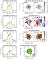 |
Fig. A.1. HCN 3–2 and HCO+ 3–2 for IRAS 17208−0014. Left panels: (Top two panels) Spectra extracted from the resolved aperture. (Lower two panels) Spectra extracted from the global aperture. Velocities are relative to the systemic velocity. The corresponding velocities of potentially detected species are indicated by vertical dotted lines. Right panels: (Top) Integrated intensity over ±500 km s−1 (moment 0). Contours are (5, 10, 20, 40, 80, 120, 160, 200, 240) ×σ, where σ is 0.096 Jy km s−1 beam−1. (Second from top) Velocity field (moment 1). Contours are in steps of ±50 km s−1. (Third from top) Velocity dispersion (moment 2). Contours are in steps of 20 km s−1. Moment 1 and 2 were derived with 3σ clipping. (Bottom) |

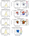 |
Fig. A.2. HCN 3–2 and HCO+ 3–2 for IRAS 09022−3615. Left panels: (Top two panels) Spectra extracted from the resolved aperture. (Lower two panels) Spectra extracted from the global aperture. Velocities are relative to the systemic velocity. The corresponding velocities of potentially detected species are indicated by vertical dotted lines. Right panels: (Top) Integrated intensity over ±500 km s−1 (moment 0). Contours are (5, 10, 20, 40, 80, 120, 160, 200) ×σ, where σ is 0.020 Jy km s−1 beam−1. (Second from top) Velocity field (moment 1). Contours are in steps of ±50 km s−1. (Third from top) Velocity dispersion (moment 2). Contours are in steps of 20 km s−1. Moment 1 and 2 were derived with 3σ clipping. (Bottom) |

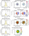 |
Fig. A.3. HCN 3–2 and HCO+ 3–2 for IRAS 13120−5453. Left panels: (Top two panels) Spectra extracted from the resolved aperture. (Lower two panels) Spectra extracted from the global aperture. Velocities are relative to the systemic velocity. The corresponding velocities of potentially detected species are indicated by vertical dotted lines. Right panels: (Top) Integrated intensity over ±500 km s−1 (moment 0). Contours are (5, 10, 20, 40, 80, 120, 160) ×σ, where σ is 0.103 Jy km s−1 beam−1. (Second from top) Velocity field (moment 1). Contours are in steps of ±50 km s−1. (Third from top) Velocity dispersion (moment 2). Contours are in steps of 20 km s−1. Moment 1 and 2 were derived with 3σ clipping. (Bottom) |

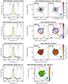 |
Fig. A.4. HCN 3–2 and HCO+ 3–2 for IRAS F14378−3651. Left panels: (Top two panels) Spectra extracted from the resolved aperture. (Lower two panels) Spectra extracted from the global aperture. Velocities are relative to the systemic velocity. The corresponding velocities of potentially detected species are indicated by vertical dotted lines. Right panels: (Top) Integrated intensity over ±250 km s−1 (moment 0). Contours are (5, 10, 20, 40, 60, 80, 100, 120, 140) ×σ, where σ is 0.019 Jy km s−1 beam−1. (Second from top) Velocity field (moment 1). Contours are in steps of ±25 km s−1. (Third from top) Velocity dispersion (moment 2). Contours are in steps of 10 km s−1. Moment 1 and 2 were derived with 3σ clipping. (Bottom) |

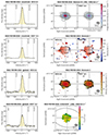 |
Fig. A.5. HCN 3–2 and HCO+ 3–2 for IRAS F05189−2524. Left panels: (Top two panels) Spectra extracted from the resolved aperture. (Lower two panels) Spectra extracted from the global aperture. Velocities are relative to the systemic velocity. The corresponding velocities of potentially detected species are indicated by vertical dotted lines. Right panels: (Top) Integrated intensity over ±250 km s−1 (moment 0). Contours are (5, 10, 20, 40, 80, 160, 240, 320, 400) ×σ, where σ is 0.024 Jy km s−1 beam−1. (Second from top) Velocity field (moment 1). Contours are in steps of ±25 km s−1. (Third from top) Velocity dispersion (moment 2). Contours are in steps of 10 km s−1. Moment 1 and 2 were derived with 3σ clipping. (Bottom) |

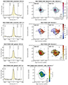 |
Fig. A.6. HCN 3–2 and HCO+ 3–2 for IRAS F10565+2448. Left panels: (Top two panels) Spectra extracted from the resolved aperture. (Lower two panels) Spectra extracted from the global aperture. Velocities are relative to the systemic velocity. The corresponding velocities of potentially detected species are indicated by vertical dotted lines. Right panels: (Top) Integrated intensity over ±250 km s−1 (moment 0). Contours are (5, 10, 20, 30, 40, 50, 60, 70, 80) ×σ, where σ is 0.023 Jy km s−1 beam−1. (Second from top) Velocity field (moment 1). Contours are in steps of ±25 km s−1. (Third from top) Velocity dispersion (moment 2). Contours are in steps of 10 km s−1. Moment 1 and 2 were derived with 3σ clipping. (Bottom) |

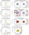 |
Fig. A.7. HCN 3–2 and HCO+ 3–2 for IRAS 19542+1110. Left panels: (Top two panels) Spectra extracted from the resolved aperture. (Lower two panels) Spectra extracted from the global aperture. Velocities are relative to the systemic velocity. The corresponding velocities of potentially detected species are indicated by vertical dotted lines. Right panels: (Top) Integrated intensity over ±300 km s−1 (moment 0). Contours are (5, 10, 20, 40, 80, 160, 240) ×σ, where σ is 0.019 Jy km s−1 beam−1. (Second from top) Velocity field (moment 1). Contours are in steps of ±25 km s−1. (Third from top) Velocity dispersion (moment 2). Contours are in steps of 10 km s−1. Moment 1 and 2 were derived with 3σ clipping. (Bottom) |

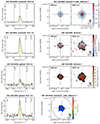 |
Fig. A.8. HCN 3–2 and HCO+ 3–2 for ESO 148−IG002. Left panels: (Top two panels) Spectra extracted from the resolved aperture. (Lower two panels) Spectra extracted from the global aperture. Velocities are relative to the systemic velocity. The corresponding velocities of potentially detected species are indicated by vertical dotted lines. Right panels: (Top) Integrated intensity over ±200 km s−1 (moment 0). Contours are (5, 10, 20, 40, 60, 80, 100) ×σ, where σ is 0.019 Jy km s−1 beam−1. (Second from top) Velocity field (moment 1). Contours are in steps of ±10 km s−1. (Third from top) Velocity dispersion (moment 2). Contours are in steps of 4 km s−1. Moment 1 and 2 were derived with 3σ clipping. (Bottom) |

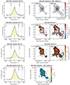 |
Fig. A.9. HCN 3–2 and HCO+ 3–2 for NGC 6240. Left panels: (Top two panels) Spectra extracted from the resolved aperture. (Lower two panels) Spectra extracted from the global aperture. Velocities are relative to the systemic velocity. The corresponding velocities of potentially detected species are indicated by vertical dotted lines. Right panels: (Top) Integrated intensity over ±500 km s−1 (moment 0). Contours are (5, 10, 20, 40, 60, 80, 100) ×σ, where σ is 0.040 Jy km s−1 beam−1. (Second from top) Velocity field (moment 1). Contours are in steps of ±50 km s−1. (Third from top) Velocity dispersion (moment 2). Contours are in steps of 20 km s−1. Moment 1 and 2 were derived with 3σ clipping. (Bottom) |

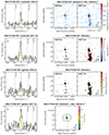 |
Fig. A.10. HCN 3–2 and HCO+ 3–2 for IRAS F17138−1017. Left panels: (Top two panels) Spectra extracted from the resolved aperture. (Lower two panels) Spectra extracted from the global aperture. Velocities are relative to the systemic velocity. The corresponding velocities of potentially detected species are indicated by vertical dotted lines. Right panels: (Top) Integrated intensity over ±150 km s−1 (moment 0). Contours are (5, 10) ×σ, where σ is 0.045 Jy km s−1 beam−1. (Second from top) Velocity field (moment 1). Contours are in steps of ±10 km s−1. (Third from top) Velocity dispersion (moment 2). Contours are in steps of 4 km s−1. Moment 1 and 2 were derived with 3σ clipping. (Bottom) |

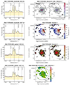 |
Fig. A.11. HCN 3–2 and HCO+ 3–2 for IRAS 17578−0400. Left panels: (Top two panels) Spectra extracted from the resolved aperture. (Lower two panels) Spectra extracted from the global aperture. Velocities are relative to the systemic velocity. The corresponding velocities of potentially detected species are indicated by vertical dotted lines. Horizontal dashed lines are the assumed continuum level. Right panels: (Top) Integrated intensity over ±250 km s−1 (moment 0). Contours are (5, 10, 20, 40, 80, 160, 320, 480, 640, 800) ×σ, where σ is 0.051 Jy km s−1 beam−1. (Second from top) Velocity field (moment 1). Contours are in steps of ±25 km s−1. (Third from top) Velocity dispersion (moment 2). Contours are in steps of 10 km s−1. Moment 1 and 2 were derived with 3σ clipping. (Bottom) |

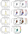 |
Fig. A.12. HCN 3–2 and HCO+ 3–2 for ESO 173−G015. Left panels: (Top two panels) Spectra extracted from the resolved aperture. (Lower two panels) Spectra extracted from the global aperture. Velocities are relative to the systemic velocity. The corresponding velocities of potentially detected species are indicated by vertical dotted lines. Right panels: (Top) Integrated intensity over ±250 km s−1 (moment 0). Contours are (5, 10, 20, 40, 80, 120, 160, 200, 240) ×σ, where σ is 0.043 Jy km s−1 beam−1. (Second from top) Velocity field (moment 1). Contours are in steps of ±25 km s−1. (Third from top) Velocity dispersion (moment 2). Contours are in steps of 10 km s−1. Moment 1 and 2 were derived with 3σ clipping. (Bottom) |

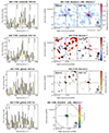 |
Fig. A.13. HCN 3–2 and HCO+ 3–2 for UGC 11763. Left panels: (Top two panels) Spectra extracted from the resolved aperture. (Lower two panels) Spectra extracted from the global aperture. Velocities are relative to the systemic velocity. The corresponding velocities of potentially detected species are indicated by vertical dotted lines. Right panels: (Top) Integrated intensity over ±200 km s−1 (moment 0). Contours are (5) ×σ, where σ is 0.018 Jy km s−1 beam−1. (Second from top) Velocity field (moment 1). Contours are in steps of ±25 km s−1. (Third from top) Velocity dispersion (moment 2). Contours are in steps of 10 km s−1. Moment 1 and 2 were derived with 3σ clipping. (Bottom) |

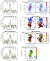 |
Fig. A.14. HCN 3–2 and HCO+ 3–2 for NGC 3110. Left panels: (Top two panels) Spectra extracted from the resolved aperture. (Lower two panels) Spectra extracted from the global aperture. Velocities are relative to the systemic velocity. The corresponding velocities of potentially detected species are indicated by vertical dotted lines. Right panels: (Top) Integrated intensity over ±200 km s−1 (moment 0). Contours are (5, 10) ×σ, where σ is 0.034 Jy km s−1 beam−1. (Second from top) Velocity field (moment 1). Contours are in steps of ±10 km s−1. (Third from top) Velocity dispersion (moment 2). Contours are in steps of 4 km s−1. Moment 1 and 2 were derived with 3σ clipping. (Bottom) |

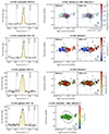 |
Fig. A.15. HCN 3–2 and HCO+ 3–2 for IC 4734. Left panels: (Top two panels) Spectra extracted from the resolved aperture. (Lower two panels) Spectra extracted from the global aperture. Velocities are relative to the systemic velocity. The corresponding velocities of potentially detected species are indicated by vertical dotted lines. Right panels: (Top) Integrated intensity over ±200 km s−1 (moment 0). Contours are (5, 10, 20, 30, 40, 50, 60) ×σ, where σ is 0.047 Jy km s−1 beam−1. (Second from top) Velocity field (moment 1). Contours are in steps of ±25 km s−1. (Third from top) Velocity dispersion (moment 2). Contours are in steps of 10 km s−1. Moment 1 and 2 were derived with 3σ clipping. (Bottom) |

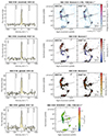 |
Fig. A.16. HCN 3–2 and HCO+ 3–2 for NGC 5135. Left panels: (Top two panels) Spectra extracted from the resolved aperture. (Lower two panels) Spectra extracted from the global aperture. Velocities are relative to the systemic velocity. The corresponding velocities of potentially detected species are indicated by vertical dotted lines. Right panels: (Top) Integrated intensity over ±150 km s−1 (moment 0). Contours are (5, 10, 15, 20, 25) ×σ, where σ is 0.049 Jy km s−1 beam−1. (Second from top) Velocity field (moment 1). Contours are in steps of ±10 km s−1. (Third from top) Velocity dispersion (moment 2). Contours are in steps of 4 km s−1. Moment 1 and 2 were derived with 3σ clipping. (Bottom) |

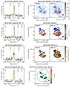 |
Fig. A.17. HCN 3–2 and HCO+ 3–2 for ESO 221−IG10. Left panels: (Top two panels) Spectra extracted from the resolved aperture. (Lower two panels) Spectra extracted from the global aperture. Velocities are relative to the systemic velocity. The corresponding velocities of potentially detected species are indicated by vertical dotted lines. Right panels: (Top) Integrated intensity over ±150 km s−1 (moment 0). Contours are (5, 10) ×σ, where σ is 0.045 Jy km s−1 beam−1. (Second from top) Velocity field (moment 1). Contours are in steps of ±10 km s−1. (Third from top) Velocity dispersion (moment 2). Contours are in steps of 4 km s−1. Moment 1 and 2 were derived with 3σ clipping. (Bottom) |

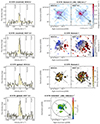 |
Fig. A.18. HCN 3–2 and HCO+ 3–2 for IC 5179. Left panels: (Top two panels) Spectra extracted from the resolved aperture. (Lower two panels) Spectra extracted from the global aperture. Velocities are relative to the systemic velocity. The corresponding velocities of potentially detected species are indicated by vertical dotted lines. Right panels: (Top) Integrated intensity over ±200 km s−1 (moment 0). Contours are (5, 10) ×σ, where σ is 0.035 Jy km s−1 beam−1. (Second from top) Velocity field (moment 1). Contours are in steps of ±10 km s−1. (Third from top) Velocity dispersion (moment 2). Contours are in steps of 4 km s−1. Moment 1 and 2 were derived with 3σ clipping. (Bottom) |

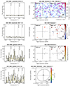 |
Fig. A.19. HCN 3–2 and HCO+ 3–2 for UGC 2982. Left panels: (Top two panels) Spectra extracted from the resolved aperture. (Lower two panels) Spectra extracted from the global aperture. Velocities are relative to the systemic velocity. The corresponding velocities of potentially detected species are indicated by vertical dotted lines. Right panels: (Top) Integrated intensity over ±150 km s−1 (moment 0). No emission is found above 5σ threshold. (Second from top) Velocity field (moment 1). Contours are in steps of ±10 km s−1. (Third from top) Velocity dispersion (moment 2). Contours are in steps of 4 km s−1. Moment 1 and 2 were derived with 3σ clipping. (Bottom) |

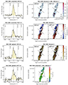 |
Fig. A.20. HCN 3–2 and HCO+ 3–2 for NGC 2369. Left panels: (Top two panels) Spectra extracted from the resolved aperture. (Lower two panels) Spectra extracted from the global aperture. Velocities are relative to the systemic velocity. The corresponding velocities of potentially detected species are indicated by vertical dotted lines. Right panels: (Top) Integrated intensity over ±300 km s−1 (moment 0). Contours are (5, 10, 15, 20, 25, 30, 35) ×σ, where σ is 0.056 Jy km s−1 beam−1. (Second from top) Velocity field (moment 1). Contours are in steps of ±25 km s−1. (Third from top) Velocity dispersion (moment 2). Contours are in steps of 10 km s−1. Moment 1 and 2 were derived with 3σ clipping. (Bottom) |

 |
Fig. A.21. HCN 3–2 and HCO+ 3–2 for ESO 286−G035. Left panels: (Top two panels) Spectra extracted from the resolved aperture. (Lower two panels) Spectra extracted from the global aperture. Velocities are relative to the systemic velocity. The corresponding velocities of potentially detected species are indicated by vertical dotted lines. Right panels: (Top) Integrated intensity over ±200 km s−1 (moment 0). Contours are (5, 10) ×σ, where σ is 0.037 Jy km s−1 beam−1. (Second from top) Velocity field (moment 1). Contours are in steps of ±25 km s−1. (Third from top) Velocity dispersion (moment 2). Contours are in steps of 10 km s−1. Moment 1 and 2 were derived with 3σ clipping. (Bottom) |

 |
Fig. A.22. HCN 3–2 and HCO+ 3–2 for ESO 320−G030. Left panels: (Top two panels) Spectra extracted from the resolved aperture. (Lower two panels) Spectra extracted from the global aperture. Velocities are relative to the systemic velocity. The corresponding velocities of potentially detected species are indicated by vertical dotted lines. Right panels: (Top) Integrated intensity over ±300 km s−1 (moment 0). Contours are (5, 10, 20, 40, 80, 160, 240, 320, 400) ×σ, where σ is 0.050 Jy km s−1 beam−1. (Second from top) Velocity field (moment 1). Contours are in steps of ±25 km s−1. (Third from top) Velocity dispersion (moment 2). Contours are in steps of 10 km s−1. Moment 1 and 2 were derived with 3σ clipping. (Bottom) |

 |
Fig. A.23. HCN 3–2 and HCO+ 3–2 for NGC 5734. Left panels: (Top two panels) Spectra extracted from the resolved aperture. (Lower two panels) Spectra extracted from the global aperture. Velocities are relative to the systemic velocity. The corresponding velocities of potentially detected species are indicated by vertical dotted lines. Right panels: (Top) Integrated intensity over ±150 km s−1 (moment 0). Contours are (5, 10) ×σ, where σ is 0.026 Jy km s−1 beam−1. (Second from top) Velocity field (moment 1). Contours are in steps of ±10 km s−1. (Third from top) Velocity dispersion (moment 2). Contours are in steps of 4 km s−1. Moment 1 and 2 were derived with 3σ clipping. (Bottom) |

Appendix B: Line ratio in the ppV space
In Sect. 5.3, we discussed the spatially and kinematically symmetric structures characterized by  exceeding the 90th percentile in each galaxy. This appendix provides a visualization of
  in the ppV space for all galaxies in which both HCN and HCO+ are significantly detected, namely, nearly the whole sample except for UGC 11763, UGC 2982, and NGC 5734.
Figure B.1 presents the ppV plots for all spaxels where both HCN and HCO+ are detected with greater than 3σ significance. Based on this figure, the sample appears to roughly split into two groups: one comprising cases where the velocity dispersion equals or exceeds any velocity gradient and another where the gas forms a low dispersion sheet exhibiting a velocity gradient. The former is predominantly found in merger cases, whereas the latter is characteristic of non-mergers (see Table 1 for merger stages).
 |
Fig. B.1. Visualization of |


Figure B.2 presents the ppV plots from the same angle as Fig. B.1 but includes only the spaxels with the line ratios higher than the 90th percentile. As discussed in the Sect. 5.3, the spatially and kinematically symmetric structures appear as a filled bicone or a thin spherical shell in the galaxies with molecular out- and/or inflows previously found by CO and/or OH line observations. Some other galaxies also (marginally) exhibit symmetric structures, possibly suggesting the presence of out- or inflows (see Appendix C for details).

Appendix C: Notes on individual galaxies
We briefly summarize previous reports of out- and inflows and discuss how they are related to the high  regions (Fig. B.2) in individual galaxies:
-
IRAS 17208-0014: García-Burillo et al. (2015) identified molecular outflows by interferometric CO 2–1 line observations and subsequent kinematic modeling. According to them, the CO outflow is likely to be a collimated conical shape elongating in the SE(blueshifted)-NW(redshifted) direction (see Fig. 18 of García-Burillo et al. 2015). In our analysis, the high
 structure appears to be a filled biconical shape whose direction of elongation is consistent with the CO results (García-Burillo et al. 2015). Inflows, as indicated by the redshifted OH absorption feature (+51 km s−1 Veilleux et al. 2013), could also contribute to elevating
  near that velocity.
 -
IRAS 09022-3615: The presence of outflows in this galaxy is suggested by the OH absorption line. The OH 119 μm absorption is shallow (∼10% relative to the continuum), possibly indicating that the outflow is significantly collimated (González-Alfonso et al. 2017). The high
 structure ambiguously appears to be a spherical shell, but its morphology seems asymmetric. It is uncertain if HCN enhancement is associated with the OH outflow.
 -
IRAS 13120-5453: In this galaxy, outflows have been found using the CO emission (Fluetsch et al. 2019; Lutz et al. 2020) and the OH absorption (Veilleux et al. 2013; González-Alfonso et al. 2017). The outflow parameters derived from these observations moderately disagree, probably due to limited signal-to-noise ratios, adopted morphology of the outflow, and excitation conditions for each molecular transition. In addition, Privon et al. (2017) reports line wings in the HCN 4–3 line as evidence for a high-velocity outflow. In our
 plots, enhancement of
  is seen in the central region at a wide range of velocities (roughly spanning [−300, +300] km s−1), possibly in the form of a collimated and nearly pole-on outflow. The high line ratio structure shows velocity reversals, which may suggest the outflow is precessing. We did not see the high-velocity components (> 300 km s−1) detected in the OH absorption, possibly due to the faintness of the HCN and HCO+ emission.
 -
IRAS F14378-3651: Molecular outflows have been detected through the blueshifted absorption feature in the far-infrared OH lines (Veilleux et al. 2013; González-Alfonso et al. 2017). According to the model by González-Alfonso et al. (2017), the OH outflows are at velocities of 250 km s−1 and 600 km s−1, located 200–300 pc away from the center. As for the CO observations, Lutz et al. (2020) found a slight flux excess at ∼250 km s−1 in the 1–0 transition, although it is not significant enough to be robust evidence for outflows. Our
 images show an enhancement in a wide-angle thin shell with a ∼250 pc radius, with the maximum velocity of ∼200 km s−1 (uncorrected for inclination). The location of the HCN enhancement seems to be associated with the lower-velocity OH outflow. On the other hand, we did not see emission from the higher-velocity (600 km s−1) outflow in our data. To detect the higher-velocity component, higher sensitivity may be required.
 -
IRAS F05189-2524: Similar to the case of IRAS F14378−3651, IRAS F05189−2524 shows an enhancement of
 , in the form of a thin spherical shell in the ppV space. In terms of velocity, the HCN-enhanced shell agrees with the lower-velocity OH outflow at 200 km s−1 reported by González-Alfonso et al. (2017). The presence of the higher-velocity (≳500 km s−1) outflows is also known by the OH absorption González-Alfonso et al. (2017) and the CO 3–2 emission (Fluetsch et al. 2019). In our observations, the line profiles of HCN and HCO+ emission show small bumps near the velocity of the fast outflow (Figs. A.5). However, the morphology of bumps are asymmetric and are likely to be affected by emission from other molecular species. Thus, the high-velocity component is not confirmed in our data.
 -
IRAS F10565+2448: The high
 regions appear to be a thin spherical shell with an ambiguous filled bicone. The highest
  is seen at velocities of ∼250 km s−1, which is consistent with the outflow velocity measured by OH absorption (Veilleux et al. 2013; González-Alfonso et al. 2017). While CO line wings in the velocity range of 300–600 km s−1 indicate the presence of faster components (Cicone et al. 2014), we did not detect emission of HCN or HCO+ in that velocity range. Higher sensitivity observations would be necessary to trace the fast components.
 -
IRAS 19542+1110: Molecular outflows in this galaxy have been found through a blueshifted OH absorption feature at the velocity of −93 km s−1 (Veilleux et al. 2013). In our analysis,
 appears to be high in a thin spherical shell with a radius of ∼500 pc and in a velocity range of about [−200, 200] km s−1. Little is known about the morphology of the outflow so far, but the structure of
  suggests that the outflow shape could be a thin shell with a wide opening angle.
 -
ESO 148-IG002: Our data show that
 is relatively low throughout the galaxy (∼0.4 on average and ∼1 at the maximum; see Table 6). Although no molecular out- or inflows are known in this galaxy so far, the highest 10th percentile in
  is in the form of a thin spherical shell with a radius of ∼500 pc and in a velocity range of about ±20 km s−1, possibly suggesting the presence of a symmetrically shaped non-circular motion.
 -
NGC 6240: Due to the interaction between the two nuclei, the kinematic structure of NGC 6240 appears to be quite complicated. The presence of outflows launched from each of the two nuclei was revealed by a detailed analysis of CO and [C I] lines (Cicone et al. 2014, 2018; Saito et al. 2018) and an OH absorption feature (Veilleux et al. 2013). The high
 regions are, however, rather randomly distributed over the entire system. We think this could be because of the disturbance by the merger. The CO and H2 line analysis (Meijerink et al. 2013) revealed that a large fraction of the gas traced by the CO J = 4–3 through 13–12 lines is affected by slow shocks, while only ≲1% traced by the H2v = 1–0 S(1) and v = 2–1 S(1) lines is exposed to the high-velocity shocks (∼17–47 km s−1). Hence the shock velocity is slow (≲10 km s−1) in the greater part of the system, no matter whether the shock is caused by a merger and/or the outflows. The shock velocity of ≲10 km s−1 is insufficient for HCN enhancement (see Sect. 6.2 for dependencies of HCN enhancement on shock velocity).
 -
IRAS F17138-1017: No dedicated study of the molecular gas distribution and kinematics was found for this galaxy. The spatial distribution of HCO+ and HCN appears to be highly asymmetric and different between these two species. While the HCO+ emission has a second peak ∼700 pc to the south of the kinematic center, the HCN emission does not. Our results suggest that there are multiple components that have different chemical compositions in the system, although we cannot specify the physical origin of the chemical diversity.
-
IRAS 17578-0400: For this galaxy, the analysis of the OH line profile suggests the presence of inflowing gas at ∼30 km s−1 (Paper I). The elongation of the HCN and HCO+ emission at low velocity may hint at an outflow along its kinematic minor axis (Paper I; Yang et al. 2023), as mentioned in Sect. 4.1. Because of the difficulty in continuum subtraction due to the line forest, it is hard to quantitatively discuss
 on a spaxel-by-spaxel basis. We tentatively analyzed
  without continuum subtraction, but it is difficult to robustly conclude that the high
  regions are related to the out- and/or inflows. To further investigate the kinematics of IRAS 17578−0400, we have conducted higher spatial resolution observations with ALMA. The detailed analysis of this observation will be presented in another paper (Yang et al., in prep.).
 -
ESO 173-G015: Although we did not find any publication on the presence of out- or inflows in this galaxy, the high
 regions were found in a symmetric shape. If we pick up the spaxels with ratios higher than the 97th percentile (> 1.402), they appear more distinctly in a thin shell. Conducting a more detailed kinematic analysis would be worthwhile in order to see if there are any outflows.
 -
UGC 11763: No publication on outflow signatures was found for this galaxy. The HCN and HCO+ emission is too faint and compact to inspect the line ratio on a spaxel-by-spaxel basis. The linewidths of the HCN and HCO+ lines seem to be much narrower than that of the CO 2–1 line (e.g., Montoya Arroyave et al. 2023, the galaxy is referred to as PG2130+099), suggesting that higher sensitivity and higher spatial resolution would be needed to grasp the molecular composition in the extended diffuse gas.
-
NGC 3110: The presence of a large-scale (≳ a few kiloparsecs) inflow is suggested by CO line observations (Kawana et al. 2022), but it is on much larger scales and not comparable to the HCN and HCO+ line-emitting region of our data. We note that
 shows some variation in the ppV space, but its structure is not very symmetrical.
 -
IC 4734: We did not find any published out- or inflow signatures.
 is distributed rather uniformly throughout the galaxy.
 -
NGC 5135: There are no known molecular out- or inflows in this galaxy. High
 can be seen in some limited small regions, but it is hard to characterize their geometry.
 -
ESO 221-IG10: No out- or inflow signature is known for this galaxy. A slight enhancement of
 can be seen in the central region, but it is only present on the blueshifted side. Higher sensitivity observations and detailed analysis of kinematics would be advisable.
 -
IC 5179: For this galaxy, we found no published signature of out- or inflows. There are some spots where
 is elevated, but they appear rather random.
 -
UGC 2982: No publication on an out- or inflow signature was found. The HCN and HCO+ emission is too faint to make any meaningful discussion.
-
NGC 2369: Although there is no published out- or inflow signature, the high
 regions are concentrated in a few 100 pc regions at the center of the galaxy. It would be worth investigating the origin of this concentration.
 -
ESO 286-G035: We did not find any publication on outflows in this galaxy. Moreover,
 does not vary much and is almost uniformly distributed throughout the galaxy.
 -
ESO 320-G030: In this galaxy, a high-velocity (450 km s−1) molecular outflow was identified by high spatial resolution observation of the CO 2–1 line (Pereira-Santaella et al. 2016). The kinematic analysis of the cited study showed that the outflow has a size of 2.5 kpc and that its blue- and redshifted regions lie in the northeast and southwest of the nucleus, respectively. Furthermore, González-Alfonso et al. (2021) found a molecular inflow associated with the nuclear bar, which is traced by the CO 2–1 line at the radius of 230–460 pc. They also pointed out that OH absorption features indicate the presence of inflowing gas at radii of 100–150 pc. We note that
 largely varies over the galaxy in the form of a characteristic structure. Most notably, the high
  regions shape a thin spherical shell with a radius of ∼100 pc. The velocity of the structure is roughly consistent with the inflows traced by the OH lines, indicating that HCN enhancement could be associated with these inflows. On the other hand, the high-velocity outflow found by Pereira-Santaella et al. (2016) is not obvious in
  in a spectrally resolved manner, but this is simply because we cannot calculate the ratio due to the faintness of the HCO+ line at high velocities. In the velocity-integrated ratio map, we may have got a hint of the enhanced
  in the outflow (Fig. A.22). The northeastern part of the outflow exhibits a considerably high
  (≳3), and the southwestern part also shows a moderately enhanced line ratio. Our subsequent ALMA observation with higher sensitivity and higher spatial resolution has clearly revealed the signature of outflow in the HCN line, and it will be presented in another paper (Gorski in prep.).
 -
NGC 5734: No published out- or inflow signature was found. We cannot discuss
 due to the faintness of the HCO+ emission over the galaxy.
All Tables
Results of the HCN 3−2 and HCO+ 3−2 line measurements: resolved and global line luminosities.
All Figures
|
Fig. 1. LIR as a function of (left) global |
| In the text | |
|
Fig. 2. Comparison of global |
| In the text | |
 |
Fig. 3. Same as Fig. 2 but for resolved |
| In the text | |
|
Fig. 4. Violin plots for |
| In the text | |
|
Fig. 5. Visualizations of |
| In the text | |
|
Fig. 6. Same as Fig. 5 but for IRAS 09022−3615, IRAS F14378−3651, IRAS F05189−2524, and IRAS F10565+2448. |
| In the text | |
 |
Fig. 7. Same as Fig. 5 but for IRAS 19542+1110 and ESO 320−G030. |
| In the text | |
|
Fig. 8. Same as Fig. 5 but for NGC 6240 and IRAS 17578−0400. We note that the continuum has not been subtracted for IRAS 17578−0400. |
| In the text | |
|
Fig. 9. One-zone non-LTE calculation of |
| In the text | |
|
Fig. 10. Chemical model predictions to simulate gas temperature, density, and fractional abundances of HCN, HCO+, and electrons under moderately-dense conditions (nH2 ∼ 103 − 104 cm−3). C-type shocks with shock velocities of 10, 20, 30, and 40 km s−1 are considered. The pre-shock H2 density is assumed to be 103 cm−2 for all cases. More details on the other assumed parameters are described in Sect. 6.2. |
| In the text | |
|
Fig. A.1. HCN 3–2 and HCO+ 3–2 for IRAS 17208−0014. Left panels: (Top two panels) Spectra extracted from the resolved aperture. (Lower two panels) Spectra extracted from the global aperture. Velocities are relative to the systemic velocity. The corresponding velocities of potentially detected species are indicated by vertical dotted lines. Right panels: (Top) Integrated intensity over ±500 km s−1 (moment 0). Contours are (5, 10, 20, 40, 80, 120, 160, 200, 240) ×σ, where σ is 0.096 Jy km s−1 beam−1. (Second from top) Velocity field (moment 1). Contours are in steps of ±50 km s−1. (Third from top) Velocity dispersion (moment 2). Contours are in steps of 20 km s−1. Moment 1 and 2 were derived with 3σ clipping. (Bottom) |
| In the text | |
|
Fig. A.2. HCN 3–2 and HCO+ 3–2 for IRAS 09022−3615. Left panels: (Top two panels) Spectra extracted from the resolved aperture. (Lower two panels) Spectra extracted from the global aperture. Velocities are relative to the systemic velocity. The corresponding velocities of potentially detected species are indicated by vertical dotted lines. Right panels: (Top) Integrated intensity over ±500 km s−1 (moment 0). Contours are (5, 10, 20, 40, 80, 120, 160, 200) ×σ, where σ is 0.020 Jy km s−1 beam−1. (Second from top) Velocity field (moment 1). Contours are in steps of ±50 km s−1. (Third from top) Velocity dispersion (moment 2). Contours are in steps of 20 km s−1. Moment 1 and 2 were derived with 3σ clipping. (Bottom) |
| In the text | |
|
Fig. A.3. HCN 3–2 and HCO+ 3–2 for IRAS 13120−5453. Left panels: (Top two panels) Spectra extracted from the resolved aperture. (Lower two panels) Spectra extracted from the global aperture. Velocities are relative to the systemic velocity. The corresponding velocities of potentially detected species are indicated by vertical dotted lines. Right panels: (Top) Integrated intensity over ±500 km s−1 (moment 0). Contours are (5, 10, 20, 40, 80, 120, 160) ×σ, where σ is 0.103 Jy km s−1 beam−1. (Second from top) Velocity field (moment 1). Contours are in steps of ±50 km s−1. (Third from top) Velocity dispersion (moment 2). Contours are in steps of 20 km s−1. Moment 1 and 2 were derived with 3σ clipping. (Bottom) |
| In the text | |
|
Fig. A.4. HCN 3–2 and HCO+ 3–2 for IRAS F14378−3651. Left panels: (Top two panels) Spectra extracted from the resolved aperture. (Lower two panels) Spectra extracted from the global aperture. Velocities are relative to the systemic velocity. The corresponding velocities of potentially detected species are indicated by vertical dotted lines. Right panels: (Top) Integrated intensity over ±250 km s−1 (moment 0). Contours are (5, 10, 20, 40, 60, 80, 100, 120, 140) ×σ, where σ is 0.019 Jy km s−1 beam−1. (Second from top) Velocity field (moment 1). Contours are in steps of ±25 km s−1. (Third from top) Velocity dispersion (moment 2). Contours are in steps of 10 km s−1. Moment 1 and 2 were derived with 3σ clipping. (Bottom) |
| In the text | |
|
Fig. A.5. HCN 3–2 and HCO+ 3–2 for IRAS F05189−2524. Left panels: (Top two panels) Spectra extracted from the resolved aperture. (Lower two panels) Spectra extracted from the global aperture. Velocities are relative to the systemic velocity. The corresponding velocities of potentially detected species are indicated by vertical dotted lines. Right panels: (Top) Integrated intensity over ±250 km s−1 (moment 0). Contours are (5, 10, 20, 40, 80, 160, 240, 320, 400) ×σ, where σ is 0.024 Jy km s−1 beam−1. (Second from top) Velocity field (moment 1). Contours are in steps of ±25 km s−1. (Third from top) Velocity dispersion (moment 2). Contours are in steps of 10 km s−1. Moment 1 and 2 were derived with 3σ clipping. (Bottom) |
| In the text | |
|
Fig. A.6. HCN 3–2 and HCO+ 3–2 for IRAS F10565+2448. Left panels: (Top two panels) Spectra extracted from the resolved aperture. (Lower two panels) Spectra extracted from the global aperture. Velocities are relative to the systemic velocity. The corresponding velocities of potentially detected species are indicated by vertical dotted lines. Right panels: (Top) Integrated intensity over ±250 km s−1 (moment 0). Contours are (5, 10, 20, 30, 40, 50, 60, 70, 80) ×σ, where σ is 0.023 Jy km s−1 beam−1. (Second from top) Velocity field (moment 1). Contours are in steps of ±25 km s−1. (Third from top) Velocity dispersion (moment 2). Contours are in steps of 10 km s−1. Moment 1 and 2 were derived with 3σ clipping. (Bottom) |
| In the text | |
|
Fig. A.7. HCN 3–2 and HCO+ 3–2 for IRAS 19542+1110. Left panels: (Top two panels) Spectra extracted from the resolved aperture. (Lower two panels) Spectra extracted from the global aperture. Velocities are relative to the systemic velocity. The corresponding velocities of potentially detected species are indicated by vertical dotted lines. Right panels: (Top) Integrated intensity over ±300 km s−1 (moment 0). Contours are (5, 10, 20, 40, 80, 160, 240) ×σ, where σ is 0.019 Jy km s−1 beam−1. (Second from top) Velocity field (moment 1). Contours are in steps of ±25 km s−1. (Third from top) Velocity dispersion (moment 2). Contours are in steps of 10 km s−1. Moment 1 and 2 were derived with 3σ clipping. (Bottom) |
| In the text | |
|
Fig. A.8. HCN 3–2 and HCO+ 3–2 for ESO 148−IG002. Left panels: (Top two panels) Spectra extracted from the resolved aperture. (Lower two panels) Spectra extracted from the global aperture. Velocities are relative to the systemic velocity. The corresponding velocities of potentially detected species are indicated by vertical dotted lines. Right panels: (Top) Integrated intensity over ±200 km s−1 (moment 0). Contours are (5, 10, 20, 40, 60, 80, 100) ×σ, where σ is 0.019 Jy km s−1 beam−1. (Second from top) Velocity field (moment 1). Contours are in steps of ±10 km s−1. (Third from top) Velocity dispersion (moment 2). Contours are in steps of 4 km s−1. Moment 1 and 2 were derived with 3σ clipping. (Bottom) |
| In the text | |
|
Fig. A.9. HCN 3–2 and HCO+ 3–2 for NGC 6240. Left panels: (Top two panels) Spectra extracted from the resolved aperture. (Lower two panels) Spectra extracted from the global aperture. Velocities are relative to the systemic velocity. The corresponding velocities of potentially detected species are indicated by vertical dotted lines. Right panels: (Top) Integrated intensity over ±500 km s−1 (moment 0). Contours are (5, 10, 20, 40, 60, 80, 100) ×σ, where σ is 0.040 Jy km s−1 beam−1. (Second from top) Velocity field (moment 1). Contours are in steps of ±50 km s−1. (Third from top) Velocity dispersion (moment 2). Contours are in steps of 20 km s−1. Moment 1 and 2 were derived with 3σ clipping. (Bottom) |
| In the text | |
|
Fig. A.10. HCN 3–2 and HCO+ 3–2 for IRAS F17138−1017. Left panels: (Top two panels) Spectra extracted from the resolved aperture. (Lower two panels) Spectra extracted from the global aperture. Velocities are relative to the systemic velocity. The corresponding velocities of potentially detected species are indicated by vertical dotted lines. Right panels: (Top) Integrated intensity over ±150 km s−1 (moment 0). Contours are (5, 10) ×σ, where σ is 0.045 Jy km s−1 beam−1. (Second from top) Velocity field (moment 1). Contours are in steps of ±10 km s−1. (Third from top) Velocity dispersion (moment 2). Contours are in steps of 4 km s−1. Moment 1 and 2 were derived with 3σ clipping. (Bottom) |
| In the text | |
|
Fig. A.11. HCN 3–2 and HCO+ 3–2 for IRAS 17578−0400. Left panels: (Top two panels) Spectra extracted from the resolved aperture. (Lower two panels) Spectra extracted from the global aperture. Velocities are relative to the systemic velocity. The corresponding velocities of potentially detected species are indicated by vertical dotted lines. Horizontal dashed lines are the assumed continuum level. Right panels: (Top) Integrated intensity over ±250 km s−1 (moment 0). Contours are (5, 10, 20, 40, 80, 160, 320, 480, 640, 800) ×σ, where σ is 0.051 Jy km s−1 beam−1. (Second from top) Velocity field (moment 1). Contours are in steps of ±25 km s−1. (Third from top) Velocity dispersion (moment 2). Contours are in steps of 10 km s−1. Moment 1 and 2 were derived with 3σ clipping. (Bottom) |
| In the text | |
|
Fig. A.12. HCN 3–2 and HCO+ 3–2 for ESO 173−G015. Left panels: (Top two panels) Spectra extracted from the resolved aperture. (Lower two panels) Spectra extracted from the global aperture. Velocities are relative to the systemic velocity. The corresponding velocities of potentially detected species are indicated by vertical dotted lines. Right panels: (Top) Integrated intensity over ±250 km s−1 (moment 0). Contours are (5, 10, 20, 40, 80, 120, 160, 200, 240) ×σ, where σ is 0.043 Jy km s−1 beam−1. (Second from top) Velocity field (moment 1). Contours are in steps of ±25 km s−1. (Third from top) Velocity dispersion (moment 2). Contours are in steps of 10 km s−1. Moment 1 and 2 were derived with 3σ clipping. (Bottom) |
| In the text | |
|
Fig. A.13. HCN 3–2 and HCO+ 3–2 for UGC 11763. Left panels: (Top two panels) Spectra extracted from the resolved aperture. (Lower two panels) Spectra extracted from the global aperture. Velocities are relative to the systemic velocity. The corresponding velocities of potentially detected species are indicated by vertical dotted lines. Right panels: (Top) Integrated intensity over ±200 km s−1 (moment 0). Contours are (5) ×σ, where σ is 0.018 Jy km s−1 beam−1. (Second from top) Velocity field (moment 1). Contours are in steps of ±25 km s−1. (Third from top) Velocity dispersion (moment 2). Contours are in steps of 10 km s−1. Moment 1 and 2 were derived with 3σ clipping. (Bottom) |
| In the text | |
|
Fig. A.14. HCN 3–2 and HCO+ 3–2 for NGC 3110. Left panels: (Top two panels) Spectra extracted from the resolved aperture. (Lower two panels) Spectra extracted from the global aperture. Velocities are relative to the systemic velocity. The corresponding velocities of potentially detected species are indicated by vertical dotted lines. Right panels: (Top) Integrated intensity over ±200 km s−1 (moment 0). Contours are (5, 10) ×σ, where σ is 0.034 Jy km s−1 beam−1. (Second from top) Velocity field (moment 1). Contours are in steps of ±10 km s−1. (Third from top) Velocity dispersion (moment 2). Contours are in steps of 4 km s−1. Moment 1 and 2 were derived with 3σ clipping. (Bottom) |
| In the text | |
|
Fig. A.15. HCN 3–2 and HCO+ 3–2 for IC 4734. Left panels: (Top two panels) Spectra extracted from the resolved aperture. (Lower two panels) Spectra extracted from the global aperture. Velocities are relative to the systemic velocity. The corresponding velocities of potentially detected species are indicated by vertical dotted lines. Right panels: (Top) Integrated intensity over ±200 km s−1 (moment 0). Contours are (5, 10, 20, 30, 40, 50, 60) ×σ, where σ is 0.047 Jy km s−1 beam−1. (Second from top) Velocity field (moment 1). Contours are in steps of ±25 km s−1. (Third from top) Velocity dispersion (moment 2). Contours are in steps of 10 km s−1. Moment 1 and 2 were derived with 3σ clipping. (Bottom) |
| In the text | |
|
Fig. A.16. HCN 3–2 and HCO+ 3–2 for NGC 5135. Left panels: (Top two panels) Spectra extracted from the resolved aperture. (Lower two panels) Spectra extracted from the global aperture. Velocities are relative to the systemic velocity. The corresponding velocities of potentially detected species are indicated by vertical dotted lines. Right panels: (Top) Integrated intensity over ±150 km s−1 (moment 0). Contours are (5, 10, 15, 20, 25) ×σ, where σ is 0.049 Jy km s−1 beam−1. (Second from top) Velocity field (moment 1). Contours are in steps of ±10 km s−1. (Third from top) Velocity dispersion (moment 2). Contours are in steps of 4 km s−1. Moment 1 and 2 were derived with 3σ clipping. (Bottom) |
| In the text | |
|
Fig. A.17. HCN 3–2 and HCO+ 3–2 for ESO 221−IG10. Left panels: (Top two panels) Spectra extracted from the resolved aperture. (Lower two panels) Spectra extracted from the global aperture. Velocities are relative to the systemic velocity. The corresponding velocities of potentially detected species are indicated by vertical dotted lines. Right panels: (Top) Integrated intensity over ±150 km s−1 (moment 0). Contours are (5, 10) ×σ, where σ is 0.045 Jy km s−1 beam−1. (Second from top) Velocity field (moment 1). Contours are in steps of ±10 km s−1. (Third from top) Velocity dispersion (moment 2). Contours are in steps of 4 km s−1. Moment 1 and 2 were derived with 3σ clipping. (Bottom) |
| In the text | |
|
Fig. A.18. HCN 3–2 and HCO+ 3–2 for IC 5179. Left panels: (Top two panels) Spectra extracted from the resolved aperture. (Lower two panels) Spectra extracted from the global aperture. Velocities are relative to the systemic velocity. The corresponding velocities of potentially detected species are indicated by vertical dotted lines. Right panels: (Top) Integrated intensity over ±200 km s−1 (moment 0). Contours are (5, 10) ×σ, where σ is 0.035 Jy km s−1 beam−1. (Second from top) Velocity field (moment 1). Contours are in steps of ±10 km s−1. (Third from top) Velocity dispersion (moment 2). Contours are in steps of 4 km s−1. Moment 1 and 2 were derived with 3σ clipping. (Bottom) |
| In the text | |
|
Fig. A.19. HCN 3–2 and HCO+ 3–2 for UGC 2982. Left panels: (Top two panels) Spectra extracted from the resolved aperture. (Lower two panels) Spectra extracted from the global aperture. Velocities are relative to the systemic velocity. The corresponding velocities of potentially detected species are indicated by vertical dotted lines. Right panels: (Top) Integrated intensity over ±150 km s−1 (moment 0). No emission is found above 5σ threshold. (Second from top) Velocity field (moment 1). Contours are in steps of ±10 km s−1. (Third from top) Velocity dispersion (moment 2). Contours are in steps of 4 km s−1. Moment 1 and 2 were derived with 3σ clipping. (Bottom) |
| In the text | |
|
Fig. A.20. HCN 3–2 and HCO+ 3–2 for NGC 2369. Left panels: (Top two panels) Spectra extracted from the resolved aperture. (Lower two panels) Spectra extracted from the global aperture. Velocities are relative to the systemic velocity. The corresponding velocities of potentially detected species are indicated by vertical dotted lines. Right panels: (Top) Integrated intensity over ±300 km s−1 (moment 0). Contours are (5, 10, 15, 20, 25, 30, 35) ×σ, where σ is 0.056 Jy km s−1 beam−1. (Second from top) Velocity field (moment 1). Contours are in steps of ±25 km s−1. (Third from top) Velocity dispersion (moment 2). Contours are in steps of 10 km s−1. Moment 1 and 2 were derived with 3σ clipping. (Bottom) |
| In the text | |
|
Fig. A.21. HCN 3–2 and HCO+ 3–2 for ESO 286−G035. Left panels: (Top two panels) Spectra extracted from the resolved aperture. (Lower two panels) Spectra extracted from the global aperture. Velocities are relative to the systemic velocity. The corresponding velocities of potentially detected species are indicated by vertical dotted lines. Right panels: (Top) Integrated intensity over ±200 km s−1 (moment 0). Contours are (5, 10) ×σ, where σ is 0.037 Jy km s−1 beam−1. (Second from top) Velocity field (moment 1). Contours are in steps of ±25 km s−1. (Third from top) Velocity dispersion (moment 2). Contours are in steps of 10 km s−1. Moment 1 and 2 were derived with 3σ clipping. (Bottom) |
| In the text | |
|
Fig. A.22. HCN 3–2 and HCO+ 3–2 for ESO 320−G030. Left panels: (Top two panels) Spectra extracted from the resolved aperture. (Lower two panels) Spectra extracted from the global aperture. Velocities are relative to the systemic velocity. The corresponding velocities of potentially detected species are indicated by vertical dotted lines. Right panels: (Top) Integrated intensity over ±300 km s−1 (moment 0). Contours are (5, 10, 20, 40, 80, 160, 240, 320, 400) ×σ, where σ is 0.050 Jy km s−1 beam−1. (Second from top) Velocity field (moment 1). Contours are in steps of ±25 km s−1. (Third from top) Velocity dispersion (moment 2). Contours are in steps of 10 km s−1. Moment 1 and 2 were derived with 3σ clipping. (Bottom) |
| In the text | |
|
Fig. A.23. HCN 3–2 and HCO+ 3–2 for NGC 5734. Left panels: (Top two panels) Spectra extracted from the resolved aperture. (Lower two panels) Spectra extracted from the global aperture. Velocities are relative to the systemic velocity. The corresponding velocities of potentially detected species are indicated by vertical dotted lines. Right panels: (Top) Integrated intensity over ±150 km s−1 (moment 0). Contours are (5, 10) ×σ, where σ is 0.026 Jy km s−1 beam−1. (Second from top) Velocity field (moment 1). Contours are in steps of ±10 km s−1. (Third from top) Velocity dispersion (moment 2). Contours are in steps of 4 km s−1. Moment 1 and 2 were derived with 3σ clipping. (Bottom) |
| In the text | |
|
Fig. B.1. Visualization of |
| In the text | |
 |
Fig. B.2. Same as Fig. B.1 but presenting spaxels with |
| In the text | |
Current usage metrics show cumulative count of Article Views (full-text article views including HTML views, PDF and ePub downloads, according to the available data) and Abstracts Views on Vision4Press platform.
Data correspond to usage on the plateform after 2015. The current usage metrics is available 48-96 hours after online publication and is updated daily on week days.
Initial download of the metrics may take a while.