| Issue |
A&A
Volume 686, June 2024
|
|
|---|---|---|
| Article Number | A213 | |
| Number of page(s) | 15 | |
| Section | The Sun and the Heliosphere | |
| DOI | https://doi.org/10.1051/0004-6361/202348314 | |
| Published online | 14 June 2024 | |
A universal method for solar filament detection from Hα observations using semi-supervised deep learning
1
Institut für Sonnenphysik (KIS), Georges-Köhler-Allee 401 A, 79110 Freiburg, Germany
e-mail: This email address is being protected from spambots. You need JavaScript enabled to view it.
2
National Solar Observatory (NSO), 3665 Discovery Drive, 80303 Boulder, CO, USA
3
Leibniz-Institut für Astrophysik Potsdam (AIP), An der Sternwarte 16, 14482 Potsdam, Germany
4
Universität Potsdam, Institut für Physik und Astronomie, Karl-Liebknecht-Straße 24/25, 14476 Potsdam, Germany
5
University of Graz, Institute of Physics, Universitätsplatz 5, 8010 Graz, Austria
6
High Altitude Observatory (HAO), 3090 Center Green Drive, 80301 Boulder, CO, USA
e-mail: This email address is being protected from spambots. You need JavaScript enabled to view it.
7
Instituto de Astrofísica de Canarias (IAC), Vía Láctea s/n, 38205 La Laguna, Tenerife, Spain
8
Departamento de Astrofísica, Universidad de La Laguna, 38205 La Laguna, Tenerife, Spain
9
Max-Planck-Institut für Sonnensystemforschung, Justus-von-Liebig-Weg 3, 37077 Göttingen, Germany
10
Astronomical Institute, Slovak Academy of Sciences, 05960 Tatranská Lomnica, Slovak Republic
11
The Applied AI Company Limited (AAICO), C11-Building 2 Al Khaleej St, Al Muntazah – Zone 1, Abu Dhabi, UAE
12
University of Graz, Kanzelhöhe Observatory for Solar and Environmental Research, Kanzelhöhe 19, 9521 Treffen am Ossiacher See, Austria
13
Skolkovo Institute of Science and Technology, Bolshoy Boulevard 30, bld. 1, Moscow 121205, Russia
Received:
18
October
2023
Accepted:
15
February
2024
Abstract
Filaments are omnipresent features in the solar atmosphere. Their location, properties, and time evolution can provide important information about changes in solar activity and assist in the operational space weather forecast. Therefore, filaments have to be identified in full-disk images and their properties extracted from these images, but manual extraction is tedious and too time-consuming, and extraction with morphological image processing tools produces a large number of false positive detections. Automatic object detection, segmentation, and extraction in a reliable manner would allow for the processing of more data in a shorter time frame. The Chromospheric Telescope (ChroTel; Tenerife, Spain), the Global Oscillation Network Group (GONG), and the Kanzelhöhe Observatory for Solar and Environmental Research (KSO; Austria) provide regular full-disk observations of the Sun in the core of the chromospheric Hα absorption line. In this paper, we present a deep learning method that provides reliable extractions of solar filaments from Hα filtergrams. First, we trained the object detection algorithm YOLOv5 with labeled filament data of ChroTel Hα filtergrams. We used the trained model to obtain bounding boxes from the full GONG archive. In a second step, we applied a semi-supervised training approach where we used the bounding boxes of filaments to train the algorithm on a pixel-wise classification of solar filaments with u-net. We made use of the increased data set size, which avoids overfitting of spurious artifacts from the generated training masks. Filaments were predicted with an accuracy of 92%. With the resulting filament segmentations, physical parameters such as the area or tilt angle could be easily determined and studied. We demonstrated this in an example where we determined the rush-to-the pole for Solar Cycle 24 from the segmented GONG images. In a last step, we applied the filament detection to Hα observations from KSO and demonstrated the general applicability of our method to Hα filtergrams.
Key words: methods: observational / methods: statistical / techniques: image processing / astronomical databases: miscellaneous / catalogs / Sun: chromosphere
© The Authors 2024
 Open Access article, published by EDP Sciences, under the terms of the Creative Commons Attribution License (https://creativecommons.org/licenses/by/4.0), which permits unrestricted use, distribution, and reproduction in any medium, provided the original work is properly cited.
This article is published in open access under the Subscribe to Open model. This email address is being protected from spambots. You need JavaScript enabled to view it. to support open access publication.
1. Introduction
Solar filaments are structures of dense, cool plasma that reach from the chromosphere into the corona and are stabilized by the magnetic field. They appear above and along the polarity inversion line, which separates large areas of opposite magnetic polarities (Martin 1998; Mackay et al. 2010). Filaments can be very dynamic objects, changing their appearance in only a few hours. If the magnetic field is destabilized, the filaments can erupt, for example, as coronal mass ejections, and the plasma stored in them is then ejected into space (Wang et al. 2020; Kuckein et al. 2020). Three kinds of filaments have been identified (Bruzek & Durrant 1977): (i) active region filaments, which are smaller, more dynamic, and rooted at large magnetic field concentrations of active regions; (ii) quiescent filaments, which appear at all latitudes and are usually larger and more stable; and (iii) intermediate filaments, where filaments are subsumed if they do not fit into the aforementioned classes (Mackay et al. 2010). A special type of quiescent filaments are polar crown filaments, which appear at high latitudes above 50° (Leroy et al. 1983). Systematic filament studies have been performed across all filament classes mainly utilizing Hα full-disk filtergrams (e.g., statistical studies by Hao et al. 2015; Pötzi et al. 2015; Diercke & Denker 2019; Chatzistergos et al. 2023). The key ingredient of all these studies is an effective extraction of the location, length, width, and other statistical properties of filaments from full-disk observations.
Automatic filament detection has been attempted in several studies mostly by employing an intensity threshold supplemented by other information (e.g., presence or absence of magnetic field neutral line, see Shih & Kowalski 2003; Qu et al. 2005; Scholl & Habbal 2008; Joshi et al. 2010; Karachik & Pevtsov 2014). Xu et al. (2018) resorted to a visual inspection of the location of polar crown filaments because they could not find a satisfactory method to extract all filaments automatically. Hao et al. (2015) applied an adaptive threshold based on the Otsu (1979) threshold but with a modification that takes into account the mean intensity on the solar disk to improve the automatic detection of filaments. Diercke & Denker (2019) extracted filaments automatically at all latitudes from synoptic charts based on Hα full-disk images by applying morphological image processing techniques. To avoid the extraction of sunspots from the data, they excluded small-scale features, which eliminated small-scale filaments as well. Moreover, the algorithm encountered problems extracting filaments at the poles in particular because the filaments were stretched in the geometrical conversion to an equidistant grid with heliographic coordinates, resulting in some artifacts in the maps.
Extracting filaments from Hα full-disk observations using conventional image processing tools is challenging due to the complexity of distinguishing them from other dark features, such as sunspots. Zhu et al. (2019, 2020) presented an approach to identify filaments from full-disk Hα images (Denker et al. 1999) obtained at the Big Bear Solar Telescope (BBSO) using the fully convolutional neural network (FCN) u-net (Ronneberger et al. 2015), which was modified to enable image segmentation to extract filaments. The authors trained the network with semi-manual computed ground truth using image manipulation software and classical image processing. The results showed an efficient segmentation compared to the classical image processing, with reduced false detection of small-scale dark objects. Nonetheless, the exclusion of sunspots is not effective in this method. Liu et al. (2021) used the same data set but with additional data from the Huairou Solar Observing Station of the National Astronomical Observatory, China (Suo 2020). With their results, they extended the comprehensive data set from Zhu et al. (2019). Another recent approach to segment filaments was presented by Ahmadzadeh et al. (2019), who used an off-the-shelf model, the Mask Region-Based Convolutional Neural Network (R-CNN; Girshick et al. 2014; He et al. 2017), and applied it to BBSO Hα full-disk data. The training data were created from maps, which were also used as input for the Heliophysics Events Knowledgebase (HEK; Hurlburt et al. 2012). In the data, non-filament regions were removed with classical morphological image processing, whose accuracy is estimated to be about 72% compared to manually labeled data (Ahmadzadeh et al. 2019). The segmentation results are comparable to the ground-truth labels and the network-identified filaments that were missing in the original HEK database. In the approach of Guo et al. (2022), the BBSO data from 2010 to 2015 was labeled with an online tool. They also included data not corrected for limb darkening and randomly varied the brightness in the training data set to improve the robustness of the segmentation method. The authors employed the CondInst (conditional convolutions for instance segmentation) model (Tian et al. 2020) for segmentation, which adeptly manages input data of various shapes and demonstrates a reliable performance across images of varying quality.
The extraction of filaments for statistical studies can be tedious. Morphological image processing is very effective, but a differentiation with other dark features on the Sun is challenging. In this study, we use a well-established deep neural network, namely, YOLOv5 (Jocher et al. 2020), with the labeled data of the Chromospheric Telescope (ChroTel; Bethge et al. 2011) to detect filaments in Hα full-disk filtergrams (Sect. 4.2). For the study of solar filaments (e.g., angle, length), a pixel-wise classification is needed. We applied a threshold per filament bounding box to provide a segmentation mask. However, in the case of extended bounding boxes, this approach may introduce artifacts and can lead to the detection of sunspots. We mitigated this shortcoming by training an additional segmentation model (i.e., u-net Ronneberger et al. 2015). To that end, we first applied the trained YOLOv5 model to the Hα filtergrams of the Global Oscillation Network Group (GONG; Harvey et al. 1996) with a four-hour cadence (17 413 observations), from which we generated our segmentation maps for the segmentation model training. We assumed that invalid segmentations appear as noise in the training data, and the detection of filaments was more robustly learned by the u-net model (c.f., Sect. 4.3). In other words, we used a semi-supervised training approach to achieve filament segmentations with reduced false detections (e.g., sunspots). The schematic outline of the present study is displayed in Fig. 1. We compared our results to the classical morphological image processing from Diercke & Denker (2019), demonstrating a clear improvement (Sect. 3.3). Afterward, the results from the different steps were evaluated (Sect. 4.1). We further applied our trained model to Hα filtergrams from the Kanzelhöhe Observatory for Solar and Environmental Research (KSO; Otruba & Pötzi 2003; Pötzi et al. 2015, 2021; Jarolim et al. 2020) in order to assess our method for Hα observations from different instruments (Sect. 5). This demonstrated that our method can extract filaments from various full-disk Hα instruments and data sources. In the end, we obtained the masks predicted by the segmentation model, and we could extract the filaments and use them as input for a statistical study similar to the one by Diercke & Denker (2019). These filaments could then be used, for example, for statistical studies with multiple applications (c.f., Sect. 6.2) or simply as input data for global databases such as HEK.
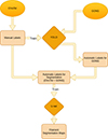 |
Fig. 1. Schematic outline of filament detection and segmentation with neural networks. |
2. Data
Our study employs Hα data from three sources: ChroTel, GONG, and KSO. In order to train a neural network to perform object detection of filaments, we labeled these filaments in Hα full-disk filtergrams. For this purpose, we used the data set of ChroTel (Kentischer et al. 2008; Bethge et al. 2011). The 10-cm aperture telescope mounted at the terrace of the VTT (von der Lühe 1998) observes in three different wavelengths, Hα, Ca II K, and He Iλ10830 Å with a cadence of 3 min. The observations were carried out with three Lyot filters, whereby the Hα filter has a full width half maximum of 0.5 Å. The regular ChroTel observations started in 2012 and continued to acquire data until 2020. The ChroTel data set contains 1056 days of observations until 2020 September, and on each day the qualitatively best filtergram was selected using the median filter-gradient similarity (MFGS; Deng et al. 2015; Denker et al. 2018) method. In this method, the similarity between the original image and the median-filtered image is evaluated. The basic data reduction includes dark- and flat-field correction as well as rotation to the solar north and geometric correction of solar images with an oval appearance, which is caused by the low elevation of the Sun in the early mornings or late evenings. Furthermore, the images were normalized to the median intensity of the solar disk, the limb darkening was corrected, and the off-limb region was truncated. The Lyot filter introduced a non-uniform intensity variation (Fig. 2, top row), which was corrected by approximation with Zernike polynomials (Shen et al. 2018). Further details of the image processing are given in Shen et al. (2018) and Diercke & Denker (2019). All filtergrams have been scaled to a solar radius of r = 1000 pixels, which results in an image scale of about 0″. 96 pixel−1 with an image size of 2000 × 2000 pixels.
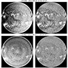 |
Fig. 2. Intensity correction of Hα ChroTel (top) and GONG (bottom) filtergrams. Left: center-to-limb-variation corrected image. Right: intensity corrected image. |
Three observers manually labeled one image of each day from the entire ChroTel data set between 2012 and 2018, which includes 955 observing days. For each image, we labeled each filament by determining the upper-left and bottom-right corner in order to construct a rectangular bounding box containing the filament. In some cases the filament was split into several parts, whereby we labeled each part individually with a bounding box. The labeled data cover observations from the maximum and minimum of Solar Cycle 24. The labels of the bounding boxes and re-scaled images with a resolution of 1024 × 1024 pixels were used as ground-truth input data for the training of the deep neural network. An example of such an input image with the corresponding labels is displayed in Fig. 3. For each red bounding box, we saved the information on the central coordinate of the box, its width, and height and the information of the type of object (class). In this study, we only have one class, namely, filaments, which has the class identifier 0.
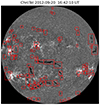 |
Fig. 3. Filtergram of Hα ChroTel with the manually labeled bounding boxes (red) for 2012 September 20. These bounding boxes define the ground-truth and input data for the object detection algorithm. |
The Global Oscillation Network Group (Harvey et al. 1996; Hill 2018) is operated by the National Solar Observatory (NSO) Integrated Synoptic Program (NISP) since 1995, with the goal being to acquire nearly continuous observations of oscillations on the solar surface. The network is comprised of six identical stations situated at different longitudes around the world, which ensures an average duty cycle of about 93% (Jain et al. 2021). The GONG instruments were designed to take full-disk observations of Doppler shifts and the line-of-sight magnetograms in the Ni I 6768 Å spectral line. In 2010, the GONG stations were upgraded to also make observations in the core of the Hα spectral line (the last system was deployed in 2010 December). The Hα instrument uses the existing GONG light feed. The GONG objective lens is 80 mm in diameter and 1000 mm in focal length. It is vignetted by the entrance turret to an effective aperture of about 70 mm, which defines the theoretical resolution of the GONG system. A polarizing beamsplitter sends light in the Hα wavelength through the Daystar Quantum PE 0.4 Å mica etalon filter. The filter is placed in a telecentric beam using two re-imaging lenses (f = 450 mm and f = 800 mm) before the filter. The filters use a unique dual-heater system developed by Daystar Filters LLC to compensate for a persistent index gradient that shifts the center wavelength across the surface of mica etalons. The filter aperture (32 mm) is matched to the GONG entrance pupil. Following the filter, two lenses (positive achromat, f = 300 mm, and negative achromat, f = −100 mm) form a Galilean telescope that creates a full-disk solar image on a Digital Video Camera Co. DVC-4000AM 2K × 2K interline uncooled CCD camera (Harvey et al. 2011). The image resolution is limited by diffraction, atmospheric seeing, and high-order wavefront errors in the filter. The diffraction-limited spatial resolution of the final image is a little over 2″. It is sampled by the CCD camera at about 1″ per pixel1.
The exposure time was adjusted automatically at each site to keep the quiet disk center at 20% of the (14-bit) dynamic range. As a first step to determining the exposure time, a pre-exposure of four images was taken with a default running average exposure time. The images were then added together and dark corrected. Flat, smear, and sky-brightness corrections were also applied. We note that the sky-brightness correction is an average brightness of the square regions of the image corners. This average brightness was then subtracted, and a corresponding scale factor was multiplied to bring the image back to a 20% dynamic range. The purpose of this correction was to compensate for known Daystar filter outgassing between maintenance visits as well as to correct for local atmospheric conditions. The resulting pre-exposure image was used to calculate the exposure time for the science image. Ten seconds later, the next four images were taken with the new pre-exposure time, applying the same dark, flat, smear, and sky-brightness corrections, and then process was repeated.
The cadence for each site is 60 s (relative to the fixed GPS time due to Universal Time leap second adjustments), but because of an (intentionally) scheduled 20-s offset in time acquisition between the neighboring sites, an overall network cadence of up to 20 s could be achieved (Jain et al. 2021). The images are 2048 × 2048 pixels in size. They were processed at each GONG site; compressed via the JPEG2000 (J2K) algorithm (with a slight loss to meet the GONG sites’ bandwidth limitations); transferred to the NISP Data Center in Boulder, Colorado; uncompressed; and made available to the public within one minute of acquisition. Because of the light feed design, the Hα images rotate during the day relative to the fixed filter and camera orientations. As part of the processing, the images were digitally de-rotated using solar ephemeris and the information about the position of GONG turrets for each site during the day. This correction is only approximate.
The GONG data was used as an additional training set for the segmentation neural network. We downloaded GONG data with a cadence of 4 h between 2010 June 01 and 2021 February 23, which resulted in a total of 17 413 images. We used the image-quality assessment method described in Jarolim et al. (2020) to filter out the observations that suffer from atmospheric degradation and exclude them from our data set. This provided a more reliable filtering of degraded images than could be achieved through quality metrics based on pixel distributions (e.g., contrast). The final GONG data set contains a total of 16 759 images. For all of our data, we used the same pre-processing to mitigate instrumental differences and enhance the image contrast. This included reduction of the image resolution to 1024 × 1024 pixels, correction of the center-to-limb-variation, and correction of additional intensity variations using Zernike polynomials (Fig. 2, bottom row), as described for ChroTel data. Finally, we clipped values to [0.8, 1.3] and then normalized the data to the interval [−1, 1].
We used additional Hα observations from KSO (KSO; Otruba & Pötzi 2003; Pötzi et al. 2015, 2021) to validate the object detection and segmentation algorithm with an additional data source. We note that KSO observes in three wavelengths: white-light, Ca II K, and Hα. The Hα observations are part of the Global Hα Network (GHN; Steinegger et al. 2000), providing Hα full-disk images on a daily basis with a cadence of about 1 min and an image scale of about 1″ pixel−1.
3. Methods
3.1. Object detection
In this section, we provide a brief introduction on object detection with deep neural networks (Elgendy 2020) and specifically on the object detection algorithm You Only Look Once (YOLO; Redmon & Farhadi 2016, 2018; Redmon et al. 2016; Jocher et al. 2020). Object detection algorithms localize an object in an image, classify each object based on the trained examples, and try to determine an optimal bounding box around the object.
One common evaluation method for object detection algorithms is Intersection over Union (IoU), which can be defined for each bounding box. The fraction of the overlap and the union of the bounding box of the ground truth BGT and the bounding box of the prediction BPred is calculated as (Elgendy 2020)
 (1)
(1)
The IoU defines the correct number of predictions, that is, the true positives (TP). Therefore, a threshold is used when a bounding box is defined as a correct prediction. The threshold for a true positive detection of a bounding box is above an IoU of 0.5; otherwise, the bounding box is considered a false positive (FP) prediction. If an object is not detected, a false negative prediction (FN) is produced. With these, we define the precision, recall, and accuracy (Elgendy 2020):
 (2)
(2)
 (3)
(3)
 (4)
(4)
where “GT" refers to the number of objects contained in the ground truth. By plotting the precision and recall values, we can define the precision-recall curve, and the area below this curve is the average precision (AP). Finally, the mean over all classes in the problem is the mAP, which is always given at a certain threshold for the IoU score. An mAP at 0.5 describes the threshold for an IoU score of 0.5.
The object detection algorithm YOLO is a single-stage detector, which means that the object class and the objectness score are predicted in the same step. This algorithm is capable of performing detections in real time, where the filament prediction is typically in the range of milliseconds on a modern GPU, which is far below the selected 60 s cadence of GONG. In YOLO, the region proposal step is omitted, and instead the image is split into grids, where for each cell a bounding box is predicted. Non-maximum suppression allows us to extract the final bounding box from the large number of candidates. There are three detection layers for detection on large, medium, and small scales. For this purpose, the image is divided into three grids of different sizes. We used YOLOv52 (Jocher et al. 2020) by Ultralytics3, which uses the Python library for deep learning applications PyTorch (Paszke et al. 2019). The model architecture is composed of three main parts: the backbone, the neck, and the head of the model. The backbone mainly extracts the important features from the input image. The neck is responsible for detecting features in the images in different scales and generalizing the model, which is performed in YOLOv5 with a feature pyramid. The model head performs the final detection. It determines the bounding boxes, the class probabilities, and objectness of the detection.
For the prediction of filament bounding boxes, we used the YOLOv5 model. To use the model for solar physics applications, we had to use a customized training of YOLOv5 from scratch, whereby the weights of the algorithm are randomly initialized, and hence no transfer learning is used. For the model architecture, we used the large configuration (c.f., Jocher et al. 2020). For the training, we used the full-disk ChroTel Hα filtergrams with a resolution of 1024 × 1024 pixels. The data set was split into a test set, a training set, and a validation set. The training set is the largest, with 681 images (70%), and the validation set contains 84 images (10%). The test set contains the remaining 192 images (20%), whereby we selected for each year one continuous block of 20% of images for the test set. The image and the corresponding file containing the coordinates of each bounding box are the input for the training of the neural network.
3.2. Segmentation
While bounding boxes allow for convenient labeling, the precise study of solar filaments requires a pixel-wise identification. As a baseline approach, we used a global intensity threshold of 1σ and selected only pixels enclosed in bounding boxes. The problem with this approach is that extended filaments and bounding boxes that overlap with sunspots lead to invalid identifications.
We built our image segmentation application on a u-net architecture (Ronneberger et al. 2015), which is a frequently employed neural network architecture for semantic segmentation. In particular, u-net is a fully convolutional network with 23 convolutional layers. The architecture is u-shaped and composed of a contracting path and an expansive path. The contracting path contains a series of convolutional layers, each followed by a rectified linear unit (ReLU) that is used to downsample the input maps. The downsampling is accompanied by the doubling of the number of feature channels. In the expansive path, the process is reversed, and with each step of the alternating convolutional layer and the ReLU, the maps are upsampled by a 2 × 2 convolution and the number of feature channels is halved. This is a concatenation with the feature maps from the contracting path.
In our study, we aim for a general method that can provide reliable solar filament detection for arbitrary Hα observations. We employed a semi-supervised approach in order to take advantage of the more robust bounding boxes and the full information of a pixel-wise segmentation. We started by training a YOLOv5 model to predict bounding boxes based on our labeled ChroTel observation. The resulting model was then used to label the full GONG archive of solar observations at a four-hour cadence, and we used an equal splitting between the available observing sites.
Using the bounding boxes of the labeled ChroTel and GONG data, we applied our thresholding approach to create a large data set of solar filament segmentations, which we used to train a final u-net model. We note that the baseline thresholding approach inevitably contains invalid pixel-wise classifications (e.g., sunspots). While noisy labels can limit the model performance, we built on the concept that for our extended data set (18 472 images), the spurious classifications are not fitted by the network. From this we expected that the neural network would not learn to replicate the noise but would focus on the task of filament classification, leading to a more reliable segmentation than the simple thresholding approach. We note that training the u-net model with only the manual labels is possible, but it does not provide a sufficiently large data set to mitigate misclassifications (e.g., the model tends to classify sunspots as filaments). For the u-net test set, we used the same continuous blocks of GONG and ChroTel observations as described in Sect. 3.1 for the training of YOLO on ChroTel data. The validation set is the same as for the YOLO training.
3.3. Setting a baseline – Segmentation with morphological image processing
To set a baseline for the performance of the machine learning algorithm, we compared the segmentation results with the results from classical morphological image processing. For this purpose, we used the ChroTel Hα filtergrams, which were corrected for intensity variations with Zernike polynomials. These filtergrams were also normalized on the median intensity. We used a threshold, which is the median intensity plus an additional 10% of the median intensity (see descriptions in Diercke & Denker 2019; Diercke et al. 2022), to create a mask of dark structures, such as filaments, for the filtergrams. In addition, we used a morphological opening and closing to create coherent contours of the filaments. As a last step, we filtered out small-scale structures with less than five pixels in order to remove non-filament structures.
4. Results
4.1. Quantitative evaluation of the results
The quantitative evaluation of the results involved a comparative analysis between the bounding boxes derived from ground-truth annotations and those predicted by YOLO for ChroTel4, alongside bounding boxes generated from segmentation maps produced by u-net and morphological image processing techniques. The data set used for the evaluation is based on all filaments predicted in each image from the test set for ChroTel data. We employed a bounding box comparison instead of a pixel-wise assessment due to the initial generation of ground-truth annotations in the bounding box format, rendering it a more convenient method of evaluation. Furthermore, our study primarily emphasizes the comprehensiveness of detection rather than the precise segmentation of individual pixels. One drawback of this approach lies in the complex handling of overlapping bounding boxes. In Fig. 4, we display an example with all utilized bounding boxes. The ground truth (light blue boxes) are the bounding boxes that were labeled manually. Since the YOLO results contain the location of the predicted bounding boxes (blue boxes), the comparison is straightforward. For the segmentation results with u-net (red boxes) and morphological image processing (yellow boxes), we had to estimate the bounding boxes around the contours. For this step, we used the regionprops routine from the Python scikit-image library. Since the bounding boxes of the ground truth always contain a certain border around the filament, the YOLO predictions mimic this behavior. For the artificially created bounding boxes around the u-net and morphological contours, we added a 20% additional height and width so that the bounding boxes could be better compared with the ground truth. For larger filaments where the width or height exceeds 50 pixels, the enlargement is 10% of the original height and width. During the labeling process, the bounding boxes tightly encapsulated the larger filaments, which is in contrast to the bounding boxes around smaller filaments. Therefore, we selected two distinct padding values, which were reasonably chosen to fit the bounding boxes from the ground truth. The bounding boxes were used to calculate the IoU, as in Eq. (1); precision, as in Eq. (2); and recall, as in Eq. (3). Thereby, a true positive could be considered when the IoU was above 10%. With the relatively low IoU score and the padded bounding boxes, our goal was to mitigate the false classification of differently separated filaments. For example, Fig. 4 shows that elongated filaments are separated into different bounding boxes by the individual methods, where we still consider the separated detections as correct. We note that the correct separation of elongated filaments would require additional information about the magnetic field topology. The results for the accuracy, precision, and recall are displayed as box plots in Fig. 5, and the corresponding statistical values are displayed in Table 1. We refrained from assessing the IoU due to this study’s primary focus on prioritizing the reliability of detection over the precise alignment of bounding boxes.
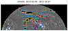 |
Fig. 4. Comparison of the bounding boxes from the ground truth (blue boxes), YOLO predictions (light blue boxes), u-net segmentation (red boxes), and segmentations using morphological image processing (yellow boxes). |
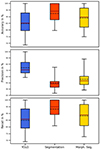 |
Fig. 5. Box plots for the accuracy, precision, and recall in percent from YOLO object detection (left, blue box), the segmentation with u-net (middle, red box), and segmentation maps obtained from morphological image processing (right, yellow box). The box is displayed between the 25th and 75th percentiles, and whiskers between the 5th and 95th percentiles. The median is marked as a dark red line and the mean as a dashed black line. |
Statistical evaluation of the accuracy, precision, and recall for object detection with YOLO, segmentation with u-net, and morphological image processing compared to the ground truth.
When evaluating the accuracy, we found the highest accuracy for the u-net segmentation, with a median value (50th percentile) of 94%. To obtain the accuracy, we compared all ground-truth bounding boxes with the number of false negative (FN) detections. A false negative detection is when we have a ground-truth bounding box but no bounding box in the predictions. This means that in most cases the u-net segmentation predicts a filament where we have a filament in the ground truth. The precision is low, with only a mean value of about 50%, which could result from a large number of false positives (FPs). False positives are defined as bounding boxes with an IoU value below the threshold of 0.1. In the false positive detections, the bounding boxes that are too small and partially overlapping with other boxes play a role. Also among the false positive detections are predicted filaments that are not present in the ground truth. The recall values of the u-net segmentation is very high, with mean values of 93%, showing that there is a very low number of false negative detections again, similar to the accuracy. The difference between the accuracy and recall of the results for morphological image processing is that much smaller contours are often predicted. In the segmentations with morphological image processing, often only a small part of the filament is detected. Then, there is a predicted bounding box within the bounding box of the ground truth with a very low IoU value so that these cases are not accounted for in the calculation of the recall values. This is especially the case when the opacity within the filament is changing. The detection with neural networks accounts for these cases much better than morphological image processing. We note that this evaluation compares the ground-truth bounding boxes with the pixel-wise segmentation of our model and therefore only provides limited information about the pixel-wise segmentation, and it can be influenced by detections of small-scale filaments (see small precision and Fig. 6).
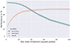 |
Fig. 6. Recall, accuracy, and precision in percent for different thresholds for the box size. |
In the following, we examine the influence of small-scale filaments predicted by the segmentation model but not labeled in the ground truth. In Fig. 6, we calculate accuracy, precision, and recall for thresholds for the bounding box areas from 2 square pixels to 100 square pixels using the predictions on the test set. In these cases, only bounding boxes with areas above the given threshold for the ground truth and the predictions by u-net were taken into account for the evaluation. Accuracy and recall decrease with higher thresholds for the bounding boxes. The precision increases mean values by about 75% for a threshold of 100 square pixels. This shows the large influence of additional predicted small-scale filaments, which are otherwise categorized as false positives.
4.2. Filament detection with YOLO
All the examples shown in the following sections from ChroTel and GONG are filtergrams from the test set. In the example in Fig. 7 (left) from 2013 March 30, we compare the ground-truth bounding boxes (blue rectangles) and the predicted bounding boxes (red rectangles). Here, most filaments have been detected by YOLO. The scattered polar crown filaments at the southern pole were detected individually as the ground truth was constructed.
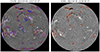 |
Fig. 7. Example for YOLO predictions on Hα filtergrams from ChroTel and GONG. Left: comparison of the ground-truth bounding boxes (blue) with predictions from YOLO (red box) for ChroTel Hα filtergrams. Right: YOLO predictions on GONG Hα filtergrams. |
In the predictions by YOLO on ChroTel data, there are single filaments with very low opacity that are labeled in the ground truth but not recognized by YOLO. However, there are also filaments that were missed in the ground truth but correctly detected by YOLO. In some cases, YOLO detected filaments that are missing in the ground truth. The precision in detecting large-scale filaments seems to be visually higher, but small-scale filaments are also well detected. In Fig. 7 (left), there are some small-scale filaments at the disk center that were not predicted by YOLO but are labeled in the ground truth. During the labeling of the filaments, filament structures with visual gaps in the spine were labeled as individual filaments. This behavior was reproduced by the YOLO detections and is especially visible in the polar crown filaments, which are often visible as scattered small-scale filamentary structures. In Fig. 7 (left), a filament was labeled individually in the ground truth, but the detection algorithm detected the filament as a single structure. Furthermore, thin clouds in the data were successfully not identified as filaments (not shown). The results also suggest that the YOLO detection algorithm effectively omitted sunspots from predictions, with bounding boxes aligning closely with the detected filaments in the majority of cases.
The process of predicting filament locations with YOLO is conveniently fast. However, the separation of filaments is subjective, and quantities such as the total area and shape of the filament are of primary importance. For this reason, we used a semi-supervised learning approach and utilized the bounding boxes to obtain pixel-wise segmentation maps. We applied the YOLO algorithm to the ChroTel data for the years 2019 and 2020, which are not labeled, and to the entire GONG data set from 2010 to 2021. The complete ChroTel and GONG data sets were used for the training of the u-net segmentation algorithm. An example of the YOLO predictions based on GONG data is shown in Fig. 7 (right). The filaments with large opacity are very well detected. Because of the differences in the spatial resolution of GONG and ChroTel data, small-scale filaments and filaments with less opacity are sometimes missed in GONG data. The polar crown filaments in the southern hemisphere are missing entirely in the example in Fig. 7 (right), and they are also less visible in the ChroTel Hα filtergrams. In contrast to the ChroTel data set, where we selected only the best image of each day, the GONG data set contains images with stronger seeing effects. In the example shown, the sunspots are successfully excluded in the detection.
One further difference between the YOLO predictions based on ChroTel data and GONG data is the prediction of the large central filament in Fig. 7. In ChroTel, the filament is labeled and predicted as one large filament, whereas in GONG it is detected as three different filaments. This is most likely due to the seeing effects in the GONG image and the different sensitivity to opacity of each instrument. The filament in GONG appears less opaque, and therefore these parts could be mistaken as a separation between different filaments by YOLO.
4.3. Segmentation of filaments using u-net
Example segmentation maps for ChroTel and GONG are displayed in Fig. 8. We selected the same examples as for the YOLO object detection in Fig. 7. Most of the filaments are well detected and segmented. All large-scale filaments were detected, but some small-scale filaments are missing. Based on the examples from the test data set, the segmentation of filaments shows better results than the object detection with YOLO. In Fig. 9, we show further examples of segmented maps with selected regions-of-interest (ROIs) of segmented active region filaments and quiet-Sun filaments. For active regions, the segmentation on the detail-rich ChroTel filtergrams is very sensitive such that penumbral filaments are sometimes detected as active region filaments. For quiet-Sun filaments, the scattered filament parts are well detected and can be used, for example, to track the filament in time (see Sect. 6.1).
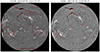 |
Fig. 8. Example for Hα filtergrams from ChroTel (left) and GONG (right). The corresponding segmentation maps from u-net are shown as red contours. |
For the segmentation of GONG, most of the filaments are successfully detected. Figure 8 (right) shows a sample segmentation map of GONG. As for the YOLO detection in Fig. 7 (right), large-scale filaments are detected, but small-scale filaments are occasionally neglected. There are even some small-scale filaments detected at the northern pole that are missing in the YOLO detection. Especially for poor seeing conditions, the segmentation of GONG data with u-net leaves out small-scale filaments. In Fig. 9, we display further examples of segmented GONG data with selected ROIs of the images. In this figure, the shapes of the filaments are also nicely preserved and represented, especially for quiet-Sun filaments. In the GONG filtergrams, less Hα fine-structure is visible; nonetheless, even here, some penumbral filaments are sometimes mistaken for filaments. For the example of 2014 September 2 (Fig. 9d), the main quiet-Sun filament is entirely detected, but on the left side of the ROI, there are some small-scale filamentary structures that were detected in the ChroTel filtergram in Fig. 9c but not in the GONG filtergram. The segmentation algorithm with u-net is able to deal with appearing clouds, such as for 2015 September 27 (Fig. 9f). In Fig. 10 (top), the large quiet-Sun filament is only partly detected by YOLO, but the segmentation with u-net has nicely segmented the entire filament (Fig. 10, bottom). This shows that the increase of the training data for the u-net also increased the reliability of the segmentation. Since YOLO was only trained on ChroTel data, the YOLO detections are not as stable as the segmentation results with u-net.
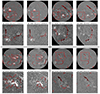 |
Fig. 9. Zoom-in of selected segmentation results with u-net for ChroTel (a, c, e, g) and GONG (b, d, f, h). The contours of the segmented filaments with u-net are in red. |
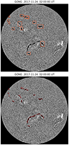 |
Fig. 10. Comparison of GONG results with YOLO (top) and u-net (bottom). |
4.4. Comparison with segmentations from morphological image processing
In Fig. 11, we display the segmentation maps created with morphological image processing (yellow contours) and compare them to the ground truth (blue boxes). As the figure shows, larger filaments with high opacity are very well detected by morphological image processing, but if the filament has different opacities, the classical algorithm misses parts of the filament or detects the filament as two structures, whereas just one filament is labeled in the ground truth. Furthermore, the thresholding method struggles with filaments that are between active regions, which have a higher intensity level. In these regions, filaments were missed more frequently. Moreover, small-scale filamentary structures are often detected as filaments where no filaments are located, as seen in Fig. 11, where there are many small contours scattered all over the solar disk. Furthermore, morphological image processing has more problems with artifacts at the solar limb.
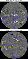 |
Fig. 11. Comparison of segmentation maps created with morphological image processing (yellow contours) with the ground truth (blue boxes) for two different days. |
5. Application on KSO images
Based on the training with data from different instruments, we expected that our neural network would be robust to instrumental variability and that it could be applied to similar Hα observations. In order to verify this, we performed a qualitative evaluation with unseen Hα data from KSO. The KSO data was processed in a manner analogous to our previous data preparation. The results of the segmentation are displayed in Fig. 12 for a sample of six filtergrams. Large-scale filaments are very well detected, as are most small-scale filaments. Similar to GONG observations, there are small-scale filaments that were not detected and other dark features that were falsely detected by the algorithm. For example, on 2015 September 27 in Fig. 12 there are clouds in the image that were successfully omitted by the algorithm. Nonetheless, there are still cases where sunspots are detected.
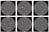 |
Fig. 12. Segmentation results from u-net for KSO images with the contours of the segmented filaments (red) for six examples of different times in the data set with different solar activity. |
When comparing the KSO images in detail with ChroTel and GONG images, we also saw slight changes in the detections. As for GONG, the KSO examples we present suffer from seeing effects, which influence the detection of small-scale filaments or effect the detection of continuous filaments as one structure. This is the case for the example on 2013 March 30 in Fig. 12 (upper-right corner), where only small parts of the filament are detected. As described in Sect. 4.2 for GONG images, the opacity is lower here than in the ChroTel images (see also Figs. 7 and 8), which could also be an effect of the different Hα filter properties. In the same example, the southern polar crown filaments are well segmented in the ChroTel (Fig. 8, left) and KSO data (Fig. 12) but not in the GONG example (Fig. 8, right), which could be due to strong seeing effects in the GONG example.
6. Sample applications of the filament segmentation
6.1. Tracking of a filament during the day
In order to test the segmentation algorithm, we applied it to a time series of an erupting filament from 2014 September 2, which is an example from the test set. The time series consists of 89 Hα observations from ChroTel taken over the day with a cadence of 3 min, although there are some gaps in the data due to bad weather conditions. In Fig. 13 (top panels), we present the segmentation for a sample of five images. The main filament is well detected, whereby the filament body contains sometimes several contours. The lift off and eruption of the filament is nicely represented in the segmentation as well. Nonetheless, in the surroundings, small-scale dark structures are detected, which are not filaments and are not constantly detected by the algorithm. This sample data set can be used to track a filament over time and study its evolution. In Fig. 13 (bottom panel), we display the evolution of the area in pixels of the filament for the same FOV as depicted in Fig. 13 (top panels). The area decreases shortly before the eruption starts, with the lift off occurring in the upper part of the filament. Afterward, the area jumps down to a much lower value, where it remains until the end of the observations.
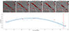 |
Fig. 13. Evolution of a giant filament on 2014 September 2 from a stable phase until its eruption. Top panels: ChroTel Hα filtergrams, tracked with the segmentation algorithm (red contours). Bottom panel: area in square pixels of the erupting filament for the observing period with ChroTel. The red circles indicate the observing times of the images in the top panels. The red vertical line indicates the start of the eruption. The blue line indicates a quadratic regression through the data points. |
6.2. Rush-to-the-pole
Segmentation maps of filaments can be used to create synoptic Carrington maps (Carrington 1858; Diercke & Denker 2019; Chatzistergos et al. 2023) for the purpose of evaluating the location of solar filaments throughout the solar cycle. This was done in the study of Diercke & Denker (2019) with ChroTel data using morphological image processing to create the segmentation maps. Here, we present an example of a statistical study to determine the rush-to-the-pole from automatically determined segmentation maps of GONG between 2010 and 2021. We created synoptic Carrington maps from the segmentation maps indicating the filament locations for Solar Cycle 24. Figure 14 displays the location of filaments on the synoptic Carrington map. In this scatter plot, we can determine the cyclic behavior of solar filaments. Around the solar cycle maximum, the number of filaments increases at low latitudes, and toward the minimum (right half of the plot), the number of filaments decreases. In the beginning of the solar cycle (left half of the plot), we can identify the rush-to-the-pole of polar crown filaments, which appear around the minimum at mid-latitudes around ±50° and appear closer to the poles toward the maximum. With the magnetic field reversal, they disappear from the solar surface.
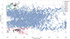 |
Fig. 14. Scatter plot of detected filaments in the GONG data set (2010–2021) for Solar Cycle 24 (blue dots). We clustered the polar regions before the magnetic field reversal with k-Means and determined the rush-to-the-pole for the northern and southern hemispheres (blue and red line, respectively). |
To determine the migration rate of polar crown filaments, we used a method similar to that of Diercke & Denker (2019), where the data points in each polar region before the magnetic field reversal are clustered and the migration rate is determined by a linear regression through all data points of the selected clusters. In the present analysis, we used the k-Means implementation from the Scikit-learn library for Python for the clustering of the filament data points. The different clusters are indicated by color in Fig. 14. For the northern hemisphere, we selected Clusters 1 and 3 and used linear regression through all data points of the clusters to determine the propagation rate. For the southern hemisphere, we used five clusters, and we selected Clusters 1, 2, and 5 for the linear regression. The results for the migration rate m are mNorth = 0.61° per rotation and mSouth = 0.84° per rotation, whereby a Carrington rotation is set as 27 days. In Diercke & Denker (2019), the migration rate for the southern hemisphere using ChroTel data was determined with m = 0.79° ±0.11° per rotation.
7. Discussion
By reviewing the results from the qualitative evaluation in Sect. 4.1, we concluded that the object detection algorithm YOLOv5 can obtain filament detections within seconds with a mean accuracy of 85%. Filaments were detected at all scales and independent of their location and opacity, including small active region filaments located in bright plage regions or close to the solar poles. Even filaments very close to the limb and erupting filaments were identified by the neural network (for example see Fig. 9). The main driver for this study was to differentiate between filaments and sunspots, which cannot be trivially solved with morphological image processing, as seen in Diercke & Denker (2019), where we excluded small-scale structures to avoid sunspots in the data, but this approach excluded small-scale filaments as well. There is a large number of polar crown filaments of small-scale that are left out. Often, a larger polar crown filament is visible as many small-scale scattered structures. In order to infer basic physical properties of filaments (e.g., location, length, width, connectivity to other layers) and perform effective statistical studies with these properties, in particular of polar crown filaments and their migration, an effective localization of filaments is of utmost importance. The segmentation with u-net enables this exact task to be performed. We were able to segment the filament completely despite changes in seeing effects. By plotting the heliographic latitude in the form of a butterfly diagram over the evolution of Solar Cycle 24, we demonstrated an easy application for the segmentation, and we could determine the rush-to-the-pole of polar crown filaments in both hemispheres (Sect. 6.2).
The YOLOv5 is a well-established detection algorithm and is easily installed and trained. The detection process is possible in real time, once the network is trained. This gives a very fast possibility to create a labeled data set with a very high precision of filament detections. The model training was only performed with observations from ChroTel. The evaluation of Hα filtergrams from GONG and KSO shows that our method can be directly applied to any new Hα data set without additional labeling efforts or model training. In order to further improve the performance of the algorithm, training with different data sources would be beneficial.
The segmentation allowed us to extract the filaments directly from the images by using the predicted masks generated by the network. In the study of Zhu et al. (2019), the trained u-net efficiently segmented the filaments, but sunspots were not excluded. The major problem was the use of a semi-manual ground truth that already contained sunspots. Other methods have been developed to separate filaments and sunspots using SVMs (Qu et al. 2005), but they require additional training and computation. Ahmadzadeh et al. (2019) used a different approach for the training data with ground-truth masks created from the HEK database, which have an accuracy of 72% compared to hand-labeled data (Ahmadzadeh et al. 2019). In our approach, we used manually labeled data and created the binary input masks from the labeled data. Sunspots are in most cases excluded, while small-scale filaments and filaments close to the limb are included in the annotations. This resulted in an optimal precondition for an effective training of the network for the segmentation of filaments. Our accuracy of the segmentation is very high, with a median value of 94%. The results justify the initial effort in manual labeling.
However, in the detail-rich ChroTel data, parts of the Hα fine-structure and penumbral filaments are sometimes detected as actual filaments. Also, sunspots are occasionally detected. In some cases, when a sunspot is detected, it is only partly segmented, particularly if other filamentary structures of an active region filament are in its proximity. Small-scale filaments are often missed in other methods because of a lack of resolution in the input data (Zhu et al. 2019; Liu et al. 2021; Guo et al. 2022). With the performed pre-processing, more small-scale filaments in ChroTel and GONG data can be recognized in the images by the presented segmentation method. Moreover, the segmentation of GONG data is stable for different seeing conditions, even if clouds cover parts of the solar disk, and it is less sensitive to instrumental differences, as can be seen from the application to the KSO data.
From Fig. 6, one can see that with a threshold of about 20 square pixels the precision largely improves to greater than 60%, while recall and accuracy marginally decrease (≈90%). Therefore, for studies that do not require small-scale filaments, a threshold of 20 square pixels is appropriate to reduce potential false positives. Nonetheless, we provide all information on the detected filaments or filamentary structures while leaving it to the scientific application of the users to filter out small-scale detections as needed.
The ground-truth labels were generated by three different people who slightly varied in the way they labeled the data. Also, after agreeing on a labeling strategy, there are cases in which more small-scale filaments are labeled, the boxes are defined as being larger than in other cases, or parts of a larger filament are labeled as one single filament, which complicates the comparison of the ground-truth bounding boxes with the segmentation results.
8. Conclusions and outlook
The presented semi-supervised learning approach using YOLO and u-net for a complete segmentation of Hα filtergrams with respect to filaments already achieves a good performance. The method can be further improved by doing the following: (1) Extending the training data of YOLO and of u-net by including the KSO data set, which is a very long-lasting data set that even contains the data of previous cycles, as it would enrich the variety of the data samples and make the training more stable. (2) Using additional wavelength channels to improve the performance of the segmentation. As KSO and ChroTel have observed Ca II-K filtergrams very close in time, these filtergrams can be used for a better differentiation between filaments and sunspots because in the Ca II K filtergrams, sunspots are more visible and typically do not display filaments. Some remnant filamentary structures are sometimes barely visible in the ChroTel filtergrams of the Ca II K line (Fig. 4 in Kuckein et al. 2016; Diercke et al. 2021). The He Iλ10 830 Å of ChroTel gives a further opportunity because the spectroscopic data allow us to use continuum observations, which only show sunspots, whereas the line-core filtergrams display sunspots and filaments, as well as plage regions as dark structures. (3) Using the HMI intensity data, with a cadence of 45 s, to exclude sunspots. False detections can be reduced by further including the line-of-sight magnetograms that contain the polarity inversion line over which each filament is formed and the strong magnetic field concentrations in the photosphere, for example in sunspots. (4) Detecting solar filaments from a video sequence rather than individual images. This could further improve the temporal consistency and mitigate seeing effects.
The filament detection and segmentation approach that we very successfully applied to the ChroTel and GONG database was also applied to KSO data. The pipeline includes a standardized automatic image reduction so that it can be used on different data sources. The pipeline including the u-net trained for filament segmentation is publicly available on GitHub5 A large-scale data integration from different telescopes will be possible, for example, for BBSO or the Uccle Solar Equatorial Telescope (USET; Clette et al. 2002). The Sun is observed by many telescopes from all over the world in Hα. Ground-based solar telescopes are restricted to observations during the day. Automated and reliable detection is required to analyze the data stream from multi-site observatories.
To foster novel research with solar filaments, we will provide catalogs based on the ChroTel and GONG data set. For ChroTel, we applied the trained segmentation method on the described ChroTel data set, that is, one image per day. The data will be available in the data archive6 of the Science Data Centre (SDC) of the Institute for Solar Physics (KIS) in Freiburg, Germany. For GONG, we applied our method to the full four-hour cadence data set. The data will be available in the Historical Solar Data archive7. The resulting pixel-wise segmentation has a high temporal cadence and high precision on the full-disk Hα filtergrams. The catalog of solar filaments enables new studies of solar filaments. For example, statistical studies of filaments over several decades can be obtained more quickly. Furthermore, the pixel-wise segmentation allows parameters such as the size or orientation of the filaments to be obtained. Moreover, the catalog paves the way for additional applications such as real-time automatic detection of eruptive filaments, which is crucial for forecasting space weather events and their potential impacts on Earth. Ultimately, it serves as a cornerstone for advancing our understanding of filament eruptions and their triggering mechanisms.
Moreover, the data can be used as an input for the HEK database, utilizing not only BBSO data (Ahmadzadeh et al. 2019) but also several instruments, with near real-time detection. Furthermore, the segmented filaments can be used as input data for another detection algorithm, that is, one that detects coronal holes (Hofmeister et al. 2019; Palacios et al. 2020; Illarionov et al. 2020; Jarolim et al. 2021) in EUV data of SDO. Filaments and coronal holes are both visible as dark objects in the solar corona, that is, in SDO observations at 193 Å. Therefore, filaments are often incorrectly detected as coronal holes. If the network learns to differentiate filaments from coronal holes, the detection of coronal holes can be improved as well (e.g., Reiss et al. 2015). In addition, the training can be extended by not only giving the location of filaments in the EUV maps but also training the data with Hα full-disk observations.
Apart from filaments, other structures can be detected with these methods. Other classes can be easily added, for example, sunspots, which are omnipresent in full-disk observations of the photosphere and chromosphere. This would require a labeled data set of sunspots to start the training, which can be created from morphological maps of dark objects that exclude the already-detected filaments. Going from full-disk images to high-resolution ground-based observations would enable many new applications of object detection and segmentation approaches based on deep learning. High-resolution observations of the High-resolution Fast Imager (HiFI; Kuckein et al. 2017; Denker et al. 2018) at the GREGOR solar telescope (Schmidt et al. 2012) are collected in a large data archive with observations in the G-band (3500 images), blue continuum (2100 images), and Ca II H (2800 images) for about 110 observing days in 2016. The labeling of the data is in progress, and implementing object detection with YOLOv8 is planned in the framework of the SOLARNET project. Since 2021, the world’s largest solar telescope, the Daniel K. Inouye Solar Telescope (DKIST, Tritschler et al. 2016; Rimmele et al. 2020), with a primary mirror of 4 m in diameter, has been regularly observing the Sun, and in the near future the European Solar Telescope (EST; Quintero Noda et al. 2022) will start operation. Therefore, a large amount of solar data (up to petabytes) will soon be collected every day with high frame rates. Deep learning algorithms for classification, object detection, and segmentation will be of utmost importance for the new era of solar observations.
The GONG Doppler velocity and magnetograph leg is further limited in its theoretical resolution to an equivalent aperture of 2.8 cm, or about 5″, sampled at 2″. 5 per pixel.
Since the selected GONG data was not simultaneously observed with the ChroTel data used to label the ground truth, the location of the filaments is slightly shifted, and a quantitative evaluation with the ground truth is not possible.
KIS Science Data Centre Archive: https://archive.sdc.leibniz-kis.de/.
Historical Solar Data archive: https://historicalsolardata.org.
Acknowledgments
The National Solar Observatory (NSO) is operated by the Association of Universities for Research in Astronomy, Inc. (AURA), under cooperative agreement with the National Science Foundation (NSF). ChroTel is operated by the Institute for Solar Physics (KIS), Freiburg, Germany, at the Spanish Observatorio del Teide, Tenerife, Canary Islands. The ChroTel filtergraph has been developed by KIS in co-operation with the High Altitude Observatory in Boulder, CO, USA. GONG Hα data were acquired by GONG instruments operated by NISP/NSO/AURA/NSF with contribution from NOAA. GONG Hα data are available at DOI: https://doi.org/10.25668/AS28-7P13. KSO Hα data were provided by the Kanzelhöhe Observatory, University of Graz, Austria. This research has received financial support from the European Union’s Horizon 2020 research and innovation program under grant agreement No. 824135 (SOLARNET). RJ acknowledges support by the SOLARNET program. AD acknowledges the SOLARNET mobility program. AAP acknowledges support by NSF grant N0017.103.OG02.UG. CK received funding from the European Union’s Horizon 2020 research and innovation programme under the Marie Skłodowska-Curie grant agreement No 895955. SJGM is grateful for the support of the European Research Council through the grant ERC-2017-CoG771310-PI2FA, by the Spanish Ministry of Science and Innovation through the grant PID2021-127487NB-I00, and by the support of the project VEGA 2/0043/24. This research has made use of NASA’s Astrophysics Data System. The authors acknowledge the use of the Skoltech Zhores cluster for obtaining the results presented in this paper (Zacharov et al. 2019).
References
- Ahmadzadeh, A., Mahajan, S. S., Kempton, D. J., Angryk, R. A., & Ji, S. 2019, ArXiv e-prints [arXiv:1912.02743] [Google Scholar]
- Bethge, C., Peter, H., Kentischer, T. J., et al. 2011, A&A, 534, A105 [NASA ADS] [CrossRef] [EDP Sciences] [Google Scholar]
- Bruzek, A., & Durrant, C. 1977, Illustrated Glossary for Solar and Solar Terrestrial Physics (Dordrecht: D. Reidel) [CrossRef] [Google Scholar]
- Carrington, R. C. 1858, MNRAS, 19, 1 [NASA ADS] [CrossRef] [Google Scholar]
- Chatzistergos, T., Ermolli, I., Banerjee, D., et al. 2023, A&A, 680, A15 [NASA ADS] [CrossRef] [EDP Sciences] [Google Scholar]
- Clette, F., Cugnon, P., Berghmans, D., van der Linden, R., & Wauters, L. 2002, in Solar Variability: From Core to Outer Frontiers, ed. A. Wilson, ESA Special Publication, 2, 935 [NASA ADS] [Google Scholar]
- Deng, H., Zhang, D., Wang, T., et al. 2015, Sol. Phys., 290, 1479 [NASA ADS] [CrossRef] [Google Scholar]
- Denker, C., Johannesson, A., Marquette, W., et al. 1999, Sol. Phys., 184, 87 [NASA ADS] [CrossRef] [Google Scholar]
- Denker, C., Dineva, E., Balthasar, H., et al. 2018, Sol. Phys., 293, 44 [NASA ADS] [CrossRef] [Google Scholar]
- Diercke, A., & Denker, C. 2019, Sol. Phys., 294, 152 [NASA ADS] [CrossRef] [Google Scholar]
- Diercke, A., Kuckein, C., Verma, M., & Denker, C. 2021, Sol. Phys., 296, 35 [NASA ADS] [CrossRef] [Google Scholar]
- Diercke, A., Kuckein, C., Cauley, P. W., et al. 2022, A&A, 661, A107 [NASA ADS] [CrossRef] [EDP Sciences] [Google Scholar]
- Elgendy, M. 2020, Deep Learning for Vision Systems (New York: Manning Publications) [Google Scholar]
- Girshick, R., Donahue, J., Darrell, T., & Malik, J. 2014, 2014 IEEE Conference on Computer Vision and Pattern Recognition, 580 [CrossRef] [Google Scholar]
- Guo, X., Yang, Y., Feng, S., et al. 2022, Sol. Phys., 297, 104 [NASA ADS] [CrossRef] [Google Scholar]
- Hao, Q., Fang, C., Cao, W., & Chen, P. F. 2015, ApJS, 221, 33 [NASA ADS] [CrossRef] [Google Scholar]
- Harvey, J. W., Bolding, J., Clark, R., et al. 2011, AAS/Solar Physics Division Meeting, 42, 17.45 [NASA ADS] [Google Scholar]
- Harvey, J. W., Hill, F., Hubbard, R. P., et al. 1996, Science, 272, 1284 [Google Scholar]
- He, K., Gkioxari, G., Dollár, P., & Girshick, R. 2017, 2017 IEEE International Conference on Computer Vision (ICCV), 2980 [CrossRef] [Google Scholar]
- Hill, F. 2018, Space Weather, 16, 1488 [NASA ADS] [CrossRef] [Google Scholar]
- Hofmeister, S. J., Utz, D., Heinemann, S. G., Veronig, A., & Temmer, M. 2019, A&A, 629, A22 [NASA ADS] [CrossRef] [EDP Sciences] [Google Scholar]
- Hurlburt, N., Cheung, M., Schrijver, C., et al. 2012, Sol. Phys., 275, 67 [Google Scholar]
- Illarionov, E., Kosovichev, A., & Tlatov, A. 2020, ApJ, 903, 115 [Google Scholar]
- Jain, K., Tripathy, S. C., Hill, F., & Pevtsov, A. A. 2021, PASP, 133, 105001 [NASA ADS] [CrossRef] [Google Scholar]
- Jarolim, R., Veronig, A. M., Pötzi, W., & Podladchikova, T. 2020, A&A, 643, A72 [NASA ADS] [CrossRef] [EDP Sciences] [Google Scholar]
- Jarolim, R., Veronig, A. M., Hofmeister, S., et al. 2021, A&A, 652, A13 [NASA ADS] [CrossRef] [EDP Sciences] [Google Scholar]
- Jocher, G., Stoken, A., Borovec, J., et al. 2020, https://doi.org/10.5281/zenodo.3983579 [Google Scholar]
- Joshi, A. D., Srivastava, N., & Mathew, S. K. 2010, Sol. Phys., 262, 425 [NASA ADS] [CrossRef] [Google Scholar]
- Karachik, N. V., & Pevtsov, A. A. 2014, Sol. Phys, 289, 821 [NASA ADS] [CrossRef] [Google Scholar]
- Kentischer, T. J., Bethge, C., Elmore, D. F., et al. 2008, in Ground-Based and Airborne Instrumentation for Astronomy II, eds. I. S. McLean, & M. M. Casali, Proc. SPIE, 7014, 701413 [NASA ADS] [Google Scholar]
- Kuckein, C., Denker, C., Verma, M., et al. 2017, in Fine Structure and Dynamics of the Solar Atmosphere, eds. S. Vargas Domínguez, A. G. Kosovichev, P. Antolin, & L. Harra, IAU Symp., 327, 20 [Google Scholar]
- Kuckein, C., Verma, M., & Denker, C. 2016, A&A, 589, A84 [NASA ADS] [CrossRef] [EDP Sciences] [Google Scholar]
- Kuckein, C., González Manrique, S. J., Kleint, L., & Asensio Ramos, A. 2020, A&A, 640, A71 [NASA ADS] [CrossRef] [EDP Sciences] [Google Scholar]
- Leroy, J. L., Bommier, V., & Sahal-Brechot, S. 1983, Sol. Phys., 83, 135 [NASA ADS] [CrossRef] [Google Scholar]
- Liu, D., Song, W., Lin, G., & Wang, H. 2021, Sol. Phys., 296, 176 [CrossRef] [Google Scholar]
- Mackay, D. H., Karpen, J. T., Ballester, J. L., Schmieder, B., & Aulanier, G. 2010, Space Sci. Rev., 151, 333 [Google Scholar]
- Martin, S. F. 1998, Sol. Phys., 182, 107 [Google Scholar]
- Otruba, W., & Pötzi, W. 2003, Hvar Obs. Bull., 27, 189 [Google Scholar]
- Otsu, N. 1979, IEEE Trans. Syst. Man Cybernet., 9, 62 [CrossRef] [Google Scholar]
- Palacios, J., Utz, D., Hofmeister, S., et al. 2020, Sol. Phys., 295, 64 [NASA ADS] [CrossRef] [Google Scholar]
- Paszke, A., Gross, S., Massa, F., et al. 2019, Advances in Neural Information Processing Systems, 8026 [Google Scholar]
- Pötzi, W., Veronig, A. M., Riegler, G., et al. 2015, Sol. Phys., 290, 951 [Google Scholar]
- Pötzi, W., Veronig, A., Jarolim, R., et al. 2021, Sol. Phys., 296, 164 [CrossRef] [Google Scholar]
- Qu, M., Shih, F. Y., Jing, J., & Wang, H. 2005, Sol. Phys., 228, 119 [NASA ADS] [CrossRef] [Google Scholar]
- Quintero Noda, C., Schlichenmaier, R., Bellot Rubio, L. R., et al. 2022, A&A, 666, A21 [NASA ADS] [CrossRef] [EDP Sciences] [Google Scholar]
- Redmon, J., & Farhadi, A. 2016, YOLO9000: Better, Faster, Stronger [Google Scholar]
- Redmon, J., & Farhadi, A. 2018, YOLOv3: An Incremental Improvement [Google Scholar]
- Redmon, J., Divvala, S., Girshick, R., & Farhadi, A. 2016, You OnlyLook Once: Unified, Real-Time Object Detection [Google Scholar]
- Reiss, M. A., Hofmeister, S. J., De Visscher, R., et al. 2015, J. Space Weather Space Clim., 5, A23 [NASA ADS] [CrossRef] [EDP Sciences] [Google Scholar]
- Rimmele, T. R., Warner, M., Keil, S. L., et al. 2020, Sol. Phys., 295, 172 [Google Scholar]
- Ronneberger, O., Fischer, P., & Brox, T. 2015, in Medical Image Computing and Computer-Assisted Intervention, eds. N. Navab, J. Hornegger, W. M. Wells, & A. F. Frangi (Cham: Springer International Publishing), 234 [Google Scholar]
- Schmidt, W., von der Lühe, O., Volkmer, R., et al. 2012, Astron. Nachr., 333, 796 [Google Scholar]
- Scholl, I. F., & Habbal, S. R. 2008, Sol. Phys., 248, 425 [NASA ADS] [CrossRef] [Google Scholar]
- Shen, Z., Diercke, A., & Denker, C. 2018, Astron. Nachr., 339, 661 [NASA ADS] [CrossRef] [Google Scholar]
- Shih, F. Y., & Kowalski, A. J. 2003, Sol. Phys., 218, 99 [NASA ADS] [CrossRef] [Google Scholar]
- Steinegger, M., Denker, C., Goode, P. R., et al. 2000, in The Solar Cycle and Terrestrial Climate, Solar and Space Weather, ed. A. Wilson, ESA Special Publication, 463, 617 [NASA ADS] [Google Scholar]
- Suo, L. 2020, Adv. Space Res., 65, 1054 [NASA ADS] [CrossRef] [Google Scholar]
- Tian, Z., Shen, C., & Chen, H. 2020, ArXiv e-prints [arXiv:2003.05664] [Google Scholar]
- Tritschler, A., Rimmele, T. R., Berukoff, S., et al. 2016, Astron. Nachr., 337, 1064 [Google Scholar]
- von der Lühe, O. 1998, New Astron. Rev., 42, 493 [Google Scholar]
- Wang, S., Jenkins, J. M., Martinez Pillet, V., et al. 2020, ApJ, 892, 75 [Google Scholar]
- Xu, Y., Pötzi, W., Zhang, H., et al. 2018, ApJ, 862, L23 [NASA ADS] [CrossRef] [Google Scholar]
- Zacharov, I., Arslanov, R., Gunin, M., et al. 2019, Open Eng., 9, 59 [Google Scholar]
- Zhu, G., Lin, G., Wang, D., Liu, S., & Yang, X. 2019, Sol. Phys., 294, 117 [CrossRef] [Google Scholar]
- Zhu, G., Lin, G., Wang, D., Liu, S., & Yang, X. 2020, in Astronomical Data Analysis Software and Systems XXIX, eds. R. Pizzo, E. R. Deul, J. D. Mol, J. de Plaa, & H. Verkouter, ASP Conf. Ser., 527, 159 [Google Scholar]
All Tables
Statistical evaluation of the accuracy, precision, and recall for object detection with YOLO, segmentation with u-net, and morphological image processing compared to the ground truth.
All Figures
|
Fig. 1. Schematic outline of filament detection and segmentation with neural networks. |
| In the text | |
|
Fig. 2. Intensity correction of Hα ChroTel (top) and GONG (bottom) filtergrams. Left: center-to-limb-variation corrected image. Right: intensity corrected image. |
| In the text | |
|
Fig. 3. Filtergram of Hα ChroTel with the manually labeled bounding boxes (red) for 2012 September 20. These bounding boxes define the ground-truth and input data for the object detection algorithm. |
| In the text | |
|
Fig. 4. Comparison of the bounding boxes from the ground truth (blue boxes), YOLO predictions (light blue boxes), u-net segmentation (red boxes), and segmentations using morphological image processing (yellow boxes). |
| In the text | |
|
Fig. 5. Box plots for the accuracy, precision, and recall in percent from YOLO object detection (left, blue box), the segmentation with u-net (middle, red box), and segmentation maps obtained from morphological image processing (right, yellow box). The box is displayed between the 25th and 75th percentiles, and whiskers between the 5th and 95th percentiles. The median is marked as a dark red line and the mean as a dashed black line. |
| In the text | |
|
Fig. 6. Recall, accuracy, and precision in percent for different thresholds for the box size. |
| In the text | |
|
Fig. 7. Example for YOLO predictions on Hα filtergrams from ChroTel and GONG. Left: comparison of the ground-truth bounding boxes (blue) with predictions from YOLO (red box) for ChroTel Hα filtergrams. Right: YOLO predictions on GONG Hα filtergrams. |
| In the text | |
|
Fig. 8. Example for Hα filtergrams from ChroTel (left) and GONG (right). The corresponding segmentation maps from u-net are shown as red contours. |
| In the text | |
|
Fig. 9. Zoom-in of selected segmentation results with u-net for ChroTel (a, c, e, g) and GONG (b, d, f, h). The contours of the segmented filaments with u-net are in red. |
| In the text | |
|
Fig. 10. Comparison of GONG results with YOLO (top) and u-net (bottom). |
| In the text | |
|
Fig. 11. Comparison of segmentation maps created with morphological image processing (yellow contours) with the ground truth (blue boxes) for two different days. |
| In the text | |
|
Fig. 12. Segmentation results from u-net for KSO images with the contours of the segmented filaments (red) for six examples of different times in the data set with different solar activity. |
| In the text | |
|
Fig. 13. Evolution of a giant filament on 2014 September 2 from a stable phase until its eruption. Top panels: ChroTel Hα filtergrams, tracked with the segmentation algorithm (red contours). Bottom panel: area in square pixels of the erupting filament for the observing period with ChroTel. The red circles indicate the observing times of the images in the top panels. The red vertical line indicates the start of the eruption. The blue line indicates a quadratic regression through the data points. |
| In the text | |
|
Fig. 14. Scatter plot of detected filaments in the GONG data set (2010–2021) for Solar Cycle 24 (blue dots). We clustered the polar regions before the magnetic field reversal with k-Means and determined the rush-to-the-pole for the northern and southern hemispheres (blue and red line, respectively). |
| In the text | |
Current usage metrics show cumulative count of Article Views (full-text article views including HTML views, PDF and ePub downloads, according to the available data) and Abstracts Views on Vision4Press platform.
Data correspond to usage on the plateform after 2015. The current usage metrics is available 48-96 hours after online publication and is updated daily on week days.
Initial download of the metrics may take a while.