| Issue |
A&A
Volume 686, June 2024
|
|
|---|---|---|
| Article Number | A260 | |
| Number of page(s) | 35 | |
| Section | Interstellar and circumstellar matter | |
| DOI | https://doi.org/10.1051/0004-6361/202347322 | |
| Published online | 18 June 2024 | |
Reconstructing the near- to mid-infrared environment in the stellar merger remnant V838 Monocerotis
1
Nicolaus Copernicus Astronomical Center, Polish Academy of Sciences,
Rabiańska 8,
87-100
Toruń, Poland
e-mail: This email address is being protected from spambots. You need JavaScript enabled to view it.
2
Université Côte d’Azur, Observatoire de la Côte d’Azur, CNRS, Laboratoire Lagrange,
06304
Nice, France
3
European Southern Observatory,
Karl-Schwarzschild-Str. 2,
85748
Garching bei Munchen, Germany
4
European Southern Observatory,
Alonso de Cordoba 3107,
Vitacura, Santiago, Chile
5
Astronomy Department, University of Michigan,
Ann Arbor, MI
48109, USA
6
Astrophysics Group, Department of Physics & Astronomy, University of Exeter,
Stocker Road,
Exeter,
EX4 4QL, UK
7
Institut de Planétologie et d’Astrophysique de Grenoble,
38058
Grenoble, France
8
The CHARA Array of Georgia State University, Mount Wilson Observatory,
Mount Wilson, CA
91203, USA
9
NASA Ames Research Center,
Moffett Field, CA
94035, USA
Received:
30
June
2023
Accepted:
25
March
2024
Abstract
Context. V838 Mon is a stellar merger remnant that erupted in a luminous red nova event in 2002. Although it has been well studied in the optical, near-infrared, and submillimeter regimes, its structure in the mid-infrared wavelengths remains elusive. Over the past two decades, only a handful of infrared interferometric studies have been performed, suggesting the presence of an elongated structure at multiple wavelengths. However, given the limited nature of these observations, the true morphology of the source has not yet been conclusively determined.
Aims. By performing image reconstruction using observations taken at the VLTI and CHARA, we aim to map out the circumstellar environment in V838 Mon.
Methods. We observed V838 Mon with the MATISSE (LMN bands) and GRAVITY (K band) instruments at the VLTI as well as the MIRCX/MYSTIC (HK bands) instruments at the CHARA array. We geometrically modelled the squared visibilities and the closure phases in each of the bands to obtain the constraints on the physical parameters. Furthermore, we constructed high-resolution images of V838 Mon in the HK bands using the MIRA and SQUEEZE algorithms to study the immediate surroundings of the star. Lastly, we also modelled the spectral features seen in the K and M bands at various temperatures.
Results. The image reconstructions show a bipolar structure that surrounds the central star in the post-merger remnant. In the K band, the super-resolved images show an extended structure (uniform disk diameter ~1.94 mas) with a clumpy morphology that is aligned along a north-west position angle (PA) of −40°. On the other hand, in the H band, the extended structure (uniform disk diameter ~1.18 mas) lies roughly along the same PA. Yet the northern lobe is slightly misaligned with respect to the southern lobe, which results in the closure phase deviations.
Conclusions. The VLTI and CHARA imaging results show that V838 Mon is surrounded by features resembling jets that are intrinsically asymmetric. This is further confirmed by the closure phase modelling. Further observations with VLTI can help to determine whether this structure shows any variations over time and also if such bi-polar structures are commonly formed in other stellar merger remnants.
Key words: instrumentation: high angular resolution / techniques: interferometric / stars: AGB and post-AGB / stars: imaging / stars: jets / stars: winds / outflows
© The Authors 2024
 Open Access article, published by EDP Sciences, under the terms of the Creative Commons Attribution License (https://creativecommons.org/licenses/by/4.0), which permits unrestricted use, distribution, and reproduction in any medium, provided the original work is properly cited.
This article is published in open access under the Subscribe to Open model. This email address is being protected from spambots. You need JavaScript enabled to view it. to support open access publication.
1 Introduction
V838 Monocerotis erupted in a luminous red nova event at the start of 2002 (Munari et al. 2002b; Tylenda 2005). Within a few weeks, it had brightened by almost two orders of magnitude to ultimately reach a peak luminosity of 106 L⊙ (Tylenda 2005; Sparks et al. 2008; Bond et al. 2003). The event is thought to have been the result of a stellar merger. According to the scenario proposed in Tylenda & Soker (2006), an 8 M⊙ B-type main sequence star coalesced with a 0.4 M⊙ young stellar object. The outburst was soon followed by a gradual decrease in temperature and its spectra soon evolved to resemble those of a late M-type supergiant (Evans et al. 2003; Loebman et al. 2015). Spectra taken in the 2000s revealed the presence of various molecules in V838 Mon, including water and transition-metal oxides (Banerjee & Ashok 2002; Kamiński et al. 2009). Dust was also observed to be produced in the post merger environment (Wisniewski et al. 2008; Kamiński et al. 2021). Additionally, a B-type companion was observed in the vicinity of the central merger remnant, which suggests that the merger had taken place in a hierarchical triple system (Munari et al. 2002a; Kamiński et al. 2021). We note that the companion was obscured by dust formed in the aftermath of the 2002 eruption (Tylenda et al. 2009). Overall, V838 Mon is the most widely studied luminous red nova in the Milky Way, although, many others have also been found within the Galaxy as well as elsewhere in the Local Group (Pastorello et al. 2019).
As the merger remnant in V838 Mon is enshrouded by dust, it is an ideal target for near to mid-infrared (NIR-MIR) inter-ferometric studies. The first of these studies was conducted by Lane et al. (2005) in which they observed V838 Mon using the Palomar Testbed Interferometer (PTI). By modelling the squared visibilities in the K-band at 2.2 μm, these authors were able to measure the size of the merger remnant of 1.83 ± 0.06 mas. There were also hints of asymmetries in the object, but due to scarce measurements these could not be confirmed. Chesneau et al. (2014) followed up these measurements between 2011 and 2014, using the Very Large Telescope Interferometer (VLTI) instruments: Astronomical Multi-BEam combineR (AMBER; Petrov et al. 2007) in the H and K bands and the MID-infrared Interferometric instrument (MIDI; Leinert et al. 2003) in the N band. Fitting uniform disk models to the AMBER measurements have given an angular diameter of 1.15 ± 0.2 mas, which (according to the authors) indicates that the photosphere in V838 Mon had contracted by about 40% over the course of a decade. Also, their modelling of the AMBER data suggests that an extended component was present in the system, with a lower limit on the full width at half maximum (FWHM) of ~20 mas. Modelling the MIDI measurements seems to point towards the presence of a dusty elongated structure whose major axis varies as a function of wavelength between 25 and 70 mas in N band. Submillimeter observations obtained with the Atacama Large Millimeter/sub millimeter Array (ALMA) in continuum revealed the presence of a flattened structure with a FWHM of 17.6 × 17.6 mas surrounding V838 Mon (Kamiński et al. 2021). Recent L band measurements by Mobeen et al. (2021) also seem to paint a similar picture. Mobeen et al. (2021) geometrically modelled the squared visibilities and closure phases in the L-band, obtained using the Multi AperTure mid-Infrared Spectroscopic Experiment instrument (MATISSE) at the VLTI in 2020. They found that the structure in the L-band is well represented by an elliptical disk tilted at an angle of −40°. Furthermore, the closure phases showed small but non-zero deviations, suggesting the presence of asymmetries in the system. The interferometric measurements span across the wavebands (from 2.2 μm to 1.3 mm) and trace a dusty structure oriented roughly along the same direction, with PA in the range of −10° (MIDI) to −50° (ALMA). This might indicate either a single overarching structure in the post-merger remnant, or multiple similarly aligned structures. Simulations of stellar merger events also suggest the presence of a disk like structure in the post-merger remnant, which is thought to be a reservoir for the pre-merger binary angular momentum (e.g. Webbink 1976; Pejcha et al. 2017).
V838 Mon serves as an excellent source with which to advance our understanding of the post-merger environment decades after a luminous red nova event. Thus, it provides us with crucial insights into the physical processes at play in these merger events and their final products in the long term. In this paper, we analyse and interpret recent interferometric observations obtained with a variety of instruments that span many NIR-MIR wavelengths.
The format of the paper is as follows. In Sect. 2 we present all of our VLTI and CHARA observations and outline the main steps of the data reduction. We also analyse and interpret recent optical speckle interferometric observations obtained at 562 and 832 nm. In Sect. 3, we mainly present the results of geometrically modelling the interferometric observables (squared visibilities and closure phases) observed with the MATISSE and GRAVITY instruments at VLTI and with MIRCX/MYSTIC at CHARA. Section 4 centres around our image reconstruction attempts for the VLTI and CHARA datasets using two distinct image reconstruction algorithms. The modelling and imaging results are discussed in depth in Sect. 5. In Sect. 6, we present the main conclusions of this study.
VLTI/GRAVITY observation log.
VLTI/MATISSE observation log.
2 Observations and data reduction
V838 Mon was observed with the VLTI located at Paranal observatory in Chile, in 2021 and 2022. Observations were carried out using the 1.8 m Auxiliary Telescopes (ATs) and two instruments, MATISSE (Lopez et al. 2022) and GRAVITY (GRAVITY Collaboration 2017). MATISSE is a four telescope beam combiner which covers the L (2.8–4.2 μm), M (4.5–5 μm), and N (8–13 μm) bands, while GRAVITY combines light in the K (1.9–2.4 μm) band. For both instruments, we intended to get 18 observing blocks (OBs) to perform our image reconstruction. However, we were only able to obtain three OBs for MATISSE and fifteen OBs for GRAVITY. The technical details of our VLTI observations are presented in Tables 1–2. In the case of MATISSE, only the large and small configurations were employed, while for GRAVITY, observations using all three configurations were carried out. In particular, intermediate configurations were also used to sample better the UV plane. The UV coverages obtained for the MATISSE and GRAVITY observations are shown in Figs. 1 and 2, respectively.
MATISSE observations were carried out in low spectral resolution (R ~ 30) using the GRA4MAT mode, whereby the GRAVITY fringe tracker was used to stabilize fringes for MATISSE (Lopez et al. 2022). Each MATISSE observation for V838 Mon consisted of a CAL-SCI-CAL observing sequence in which two calibrator stars, 20 Mon (spectral type K0 III) and HD 52666 (spectral type K5 III), were observed to calibrate the LMN bands. The source and calibrator fluxes in the LMN bands are given in Table 3.
The GRAVITY observations were carried out in medium spectral resolution (R ~ 500) using its single-field mode in which the light is split equally between the fringe tracker channel and the science channel. We adopted a CAL-SCI-CAL sequence for each GRAVITY run. However, one calibrator was observed here, HD 54990 (spectral type K0/1 III).
Interferometric observations of V838 Mon were also obtained at the Center for High Angular Resolution Astronomy (CHARA) array on UT 2022 March 2, 3, and 9. The UV coverage for these observations are shown in Fig. 3. The CHARA array is operated by Georgia State University and is located at Mount Wilson Observatory in southern California. The array consists of six 1-meter telescopes arranged in a Y-configuration with baselines ranging in length from 34 m to 331 m (ten Brummelaar et al. 2005). We combined the light from four to five of the telescopes using the Michigan InfraRed Combiner-eXeter (MIRC-X) beam combiner in the H-band using the low spectral resolution (R = 50) prism that disperses light over eight spectral channels (Anugu et al. 2020). On the last night, additional simultaneous observations were obtained using the Michigan Young STar Imager (MYSTIC) combiner (Setterholm et al. 2022) in the K band in the low spectral resolution (R = 49) mode (Monnier et al. 2018). The CHARA MIRC-X and MYSTIC observation log is given in Table 4. On each night, we alternated between observations of V838 Mon and calibrator stars to calibrate the interferometric transfer function. The H band fluxes are presented in Table 5, while the uniform disk diameters of the calibrators in the HK bands were adopted from Bourgés et al. (2014) and Bourgés et al. (2017) and are listed in Table 6.
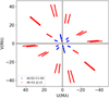 |
Fig. 1 UV tracks for MATISSE observing runs in 2021–2022. |
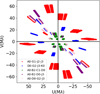 |
Fig. 2 UV coverage for GRAVITY observing runs. |
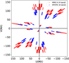 |
Fig. 3 UV coverage for CHARA observing runs in the HK bands. |
Total LMN band fluxes of V838 Mon and the calibrators.
CHARA observation log.
Total H band fluxes of V838 Mon and the calibrator.
H band calibrator uniform disk diameters.
2.1 MATISSE data reduction
The LMN-band MATISSE data were reduced using version 1.7.5 of the ESO data reduction pipeline. It carries out in parallel two types of processing: an ‘incoherent one’ that produces dispersed squared visibilities and closure phases, and a ‘coherent’ one that produces dispersed visibilities (hereafter referred to as linear visibilities) and differential phases (see Lopez et al. 2022). The uncalibrated observables are stored in OIFITS files (version 2). Per exposure, we obtained six dispersed squared visibilities, three independent closure phases, six dispersed visibilities and differential phases1, and four total spectra. A single MATISSE exposure lasts 60 s. We refer to Mobeen et al. (2021) for more details on the MATISSE observing sequence, which includes a series of exposures taken without and with chopping; the chopping being used to estimate and remove more accurately the thermal background contribution from the photometric measurements in the LM band and especially in the N band. The observations of V838 Mon were then calibrated using our measurements of the calibrator stars listed in Table 3, whose diameters and fluxes were taken from the JMMC Stellar Diameter Catalog version 2 (Chelli et al. 2016) and the Mid-infrared stellar Diameters and Fluxes compilation Catalog2 (MDFC; Cruzalebes et al. 2019, see Table 2). The calibration of squared visibilities and linear visibilities was performed by dividing the raw squared and linear visibilities of V838 Mon by those of the calibrators, corrected for their diameter (called the interferometric transfer function). The calibrated LMN spectra of V838 Mon were obtained by multiplying the ratio between the target and calibrator raw fluxes measured by MATISSE, for each telescope, at each wavelength by a model of the absolute flux of the calibrator. This model was taken from the PHOENIX stellar spectra grid (Husser et al. 2013). The final calibrated spectra were then obtained by averaging over the four telescopes. A final calibration step was the merging of the different exposures of each snapshot to produce our final visibilities, closure phases, and total spectra.
Upon completing the data reduction and inspecting the resultant products, we considered only the chopped data in the LM bands because of the more accurate photometry estimation associated with chopping. In the N band, we found that the squared visibilities were of poor quality. This was because the average N-band total flux of V838 Mon (~15 Jy) lies very close to the photometric sensitivity limit of MATISSE in the N-band, especially beyond 11 μm due to the increased thermal background effects. Moreover, the N-band correlated flux level (~5 Jy) turns out to be slightly greater than the sensitivity limit of the GRA4MAT mode in N-band. In such a situation, we thus discarded the squared visibilities and considered instead the linear visibilities, which are usually less noisy in such a low-flux regime in the N band.
Total K band fluxes of V838 Mon and the calibrator.
2.2 GRAVITY data reduction
The GRAVITY data reduction was performed with the ESO GRAVITY data reduction pipeline version 1.4.1 This was carried out in the ESO Reflex workflow environment. For the calibration of squared visibilities, we used the visibility calibration workflow in Reflex. The K data were calibrated using the calibrator star HD 54990 (see Table 7). Furthermore, the reduced K band spectra were flux calibrated similarly to the L band spectra obtained from MATISSE. The flux calibration routine from the MATISSE consortium was used for this purpose and, just as in the case of the M band, the K band spectra were also similarly normalized and later compared to synthetic spectra.
2.3 CHARA data reduction
The CHARA data were reduced and calibrated by the support astronomers at the CHARA array. The data were reduced using the standard MIRC-X and MYSTIC pipeline (version 1.3.5) written in python3 and described by Anugu et al. (2020). The pipeline produces calibrated visibility amplitudes for each pair of telescopes and closure phases for each combination of three telescopes. To assess the data quality, the calibrators were checked against each other on each night. The calibrators showed no evidence for binarity based on a visual inspection of the data, and the diameters derived from the measured visibilities were consistent with the expected values within uncertainties. The calibrated OIFITS files will be available in the Optical Interferometry Database4 and the CHARA Data Archive5.
2.4 Gemini South observation
V838 Mon was also observed twice with the Gemini South 8-m telescope using the high-resolution Zorro instrument (Scott et al. 2021; Howell & Furlan 2022). Zorro provides simultaneous speckle imaging in two optical bands, centered here at 562 nm and 832 nm. V838 Mon was observed on 25 Feb. 2021 UT and, about one year later, on 20 March 2022 UT. The speckle imaging on each night consisted of a number of 60 ms frames taken in a row, the February 2021 observation taking 12 000 frames and the March 2022 observation taking 16000 frames. The February observations occurred during a night of average seeing (0″.6) while the longer March 2022 observations occurred during good seeing (0″.45). The data were reduced using a standard speckle imaging pipeline with reduced output data products including reconstructed images and 5σ contrast limits (Howell et al. 2011). The two sets of observations agreed well with the March 2022 data, providing a higher S/N result.
Figure 4 shows the 832 nm reconstructed image from March 2022, while Fig. 5 shows a similar reconstructed image but for February 2021 at 562 nm. There are no close (<1″.2) stellar companions detected within the angular and contrast limits achieved. However, as seen in Fig. 4, the image at 832 nm is extended beyond just a point source with a slight elongation in the north-south direction and to the east by about 0″.03. Similarly, at 562 nm, we also see a noticeable elongation in the northwestern direction, as shown in Fig. 5. The 562 nm elongation is in very good agreement with what we observe in the HKLMN bands (see Fig. 6). While the elongation varies significantly at 832 nm, we note that the orientation (north-south) of this particular structure is remarkably similar to the PA (~3°) we obtain by fitting the N band visibility amplitudes with an elliptical disk model. It is only with future extensive observations at Gemini South that it will be possible to reliably constrain the orientation of the elongation of V838 Mon in the V and I bands.
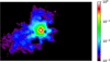 |
Fig. 4 Speckle image reconstruction from March 2022 at 832 nm. A noticeable north-south elongation is visible. The image field of view (FoV) is 0″.85 by 0″.755. North is up, east is left. The lowest reliable emission feature is at 10% of the peak intensity level. |
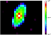 |
Fig. 5 Speckle image reconstruction from February 2021 at 562 nm. A prominent north-west elongation is visible. The image FoV is 0″.21 by 0″.14. North is up, east is left. The lowest reliable emission feature is at 10% of the peak intensity level. |
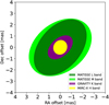 |
Fig. 6 Sketch of the best fitting elliptical models for V838 Mon in the HKL bands, as observed by MIRC-X, GRAVITY, and MATISSE. |
3 Geometrical modelling
The resultant data products for the above-mentioned VLTI and CHARA instruments are the interferometric observables, namely, the squared visibilities (V2) and closure phases. The squared visibilities represent the fringe contrast; thus, an object is said to be completely resolved in the case that the value for the squared visibility is zero, and completely unresolved in the case the value is one. The squared visibilities can be used to constrain the size of the source. Closure phases are the sum of the individual phase measurements by telescopes within a particular triangular configuration in the array. This results in the cancelling out of the atmospheric phase, namely, the phase of the complex visibility function is sensitive to the object symmetry (Jennison 1958). Therefore, the closure phases are a probe for asymmetries, so deviations from values of 0° or 180° would indicate some deviation from the centro-symmetry of the source.
3.1 L-band geometrical modelling (MATISSE)
Previous geometrical modelling and preliminary imaging results in the L band seem to suggest the presence of an elongated and tilted structure that enshrouds the central merger remnant (Mobeen et al. 2021). The VLTI observations in 2020 were obtained using only the large configuration. In the current study, V838 Mon was observed with the small (maximal baseline is ≈30 m) and large (minimal baseline ≈140 m) configurations in the L band. A quick look at the squared visibilities as a function of spatial frequency suggests that the source is mostly resolved at the longer baselines (see Fig. 7). However, even with the most extended array configuration, V838 Mon is not completely resolved as the squared visibilities drop to a minimum of about 0.3. At the shortest baselines, V838 Mon is mostly unresolved, with the squared visibilities being at around 0.9. As a function of wavelength, however, it is clear that the squared visibilities do not show much variation over most of the L band. However, we do see slight variation in the squared visibilities at the endpoints of the wavebands (see Fig. B.1). For instance, there is a slow rise until at about 3.25 μm, after which the squared visibilities remain constant and then start to fall again beyond 3.8 μm. It is not immediately obvious what could be the cause for this behavior of the squared visibilities. We rule out any miscalibrations given the quality of our calibrator data. It could be the case that what we are seeing at the edges of the L band could be due to the presence of spectral features such as H2O below 3.4 μm and SiO in its first overtone near 4 μm. If true, this would mean that the changing squared visibilities are indicative of the different sizes of the distinct emission regions. Due to scarce data at the band edges as well as the relatively unresolved flux (as suggested by the squared visibilities), we could not perform geometrical model fitting to these data points. For consistency purposes, we restricted ourselves to the wavelength range of 3–4 μm in the L band, which was the exact wavelength range considered in Mobeen et al. (2021). This allowed for a direct comparison to the previous L band results.
A qualitative look at the closure phases (see Fig. B.2) indicates that they are mostly close to zero, with some very small deviations of about a few degrees (maximum ~3°) and a mean error of ~1°. This suggests a slight asymmetry in the system. Again, similar to the squared visibilities we do not see much variation in the closure phases as a function of wavelength, except just slightly at the endpoints (see Fig. B.1).
To interpret the MATISSE data, we employed geometrical modelling, because the UV coverage of the MATISSE 2021/2022 data alone is insufficient for comprehensive imaging. We used the modelling software LITPRO provided by Jean-Marie Mariotti Center6 (JMMC), which allows the user to fit simple geometrical models such as disks, point sources and ellipses to the observed visibilities and closure phases. LITpro uses a χ2 minimization scheme to compute the model parameters and their error bars. The parameter errors were obtained from the diagonal of the calculated covariance matrix, which were then re-scaled by the square root of the final χ2 value7. For the purpose of fitting the V838 Mon data, we tried four models: a uniform circular disk (CD), an elliptical disk (ED), a circular Gaussian, and an elliptical Gaussian. With a reduced χ2 of 6, we found the elliptical models to better represent the data. The plots of the modelled and observed visibilities are shown in Fig. 7. Additionally, we are able to obtain estimates for the size and PA for the various models. These are listed in the Table A.1. The obtained parameters for size and orientation are in good agreement with what previous MATISSE observations had indicated (Mobeen et al. 2021). In Mobeen et al. (2021), the elliptical disk model yielded a semi-major axis PA of −40° ± 6°, an angular diameter of 3.28 ± 0.18 mas, and a stretch ratio of 1.40 ± 0.1. In this study, we obtained values of −41°34±0°49, 3.69 ± 0.02 mas, and 1.56 ± 0.01, respectively. It is evident that these parameters have remained largely the same between January and March 2020 and October 2021 and March 2022. This means that the feature in the L band is non-transient on a timescale of years. The absence of any change in PA also suggests that no dynamical variations have occurred in the post merger environment since the previous size estimates made by Mobeen et al. (2021). Thus, it would seem that the disk-like feature is stable and long-lived in the L band. This allowed us to combine the two datasets and attempt imaging (see Sect. 4.1).
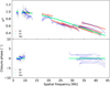 |
Fig. 7 Observed (blue) and best fits for the L band squared visibilities and closure phases. The models ED and CD refer to elliptical disk and circular disk, respectively. |
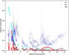 |
Fig. 8 Observations (blue) and best fit models for the N band visibility amplitudes. The models ED and CD refer to elliptical disk and circular disk, respectively. |
3.2 N-band geometrical modelling (MATISSE)
We modelled the N band visibility amplitudes in a similar way to the geometrical modelling we did for the squared visibilities in other bands. Given the scarce number of data points, we used simple geometries to model the observables. In the N band, our goal was to estimate physical parameters for the structure such as size, position angle and ellipticity under the assumption of particular geometries. This model fitting serves as a follow up to the parameter estimation in the N band performed by Chesneau et al. (2014) nearly a decade ago, where they also used similar models. We used two models, involving: a uniform disk and an elliptical disk. The uniform disk model fit yields an angular diameter of 87.73 ± 0.01 mas, while the elliptical disk model yields an angular diameter of 48.70 ± 2.40 mas, a PA of 5°.03±0°70, and a stretch ratio of 5.68 ± 0.31. These fits are shown in Fig. 8. If we consider the size estimate obtained from the elliptical disk model (semi-major axis of ~300 mas), then it would seem that the most extended structure surrounding V838 Mon exists in the N band. The PA points to a north-south elongation in the structure, which is drastically different from that seen in other bands. This means that the N band structure is a distinct feature that may not be dynamically related to structures seen in the HKL bands.
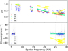 |
Fig. 9 Observations (blue) and best fit models for the M band squared visibilities and closure phases. Models ED, CD, and 2P refer to elliptical disk, circular disk, and two point sources, respectively. The angular diameters for the CD and ED models are 5.86 ± 0.08 and 4.35 ± 0.09 mas. These size estimates (4–6 mas) most likely represent the dominant circumstellar component. |
3.3 M-band geometrical modelling (MATISSE)
For the first time, we were able to observe V838 Mon in the M band using MATISSE. However, due to the scarcity of data in this band, we did not attempt any image reconstruction. As can be seen in Fig. 9, the shape of the squared visibilities as a function of spatial frequency shows a sinusoidal-like modulation. This modulation persists at all baselines and it is unlikely to be an artefact given that any telluric features and systematic effects were removed via calibration. Also, the calibrator star HD 52666 possesses no such feature which rules out the feature being a systematic error. It is prominent across all spatial frequencies, but it becomes more noticeable at longer baselines. The amplitude variation lies in the range of 0.3–0.4, while the frequency of these modulations increases at lower spatial frequencies. The M-band closure phases are mostly close to zero. However, at larger spatial frequencies, they tend to deviate by a few degrees (maximum ~5°); therefore, this hints towards asymmetries akin to those we see in the L-band.
The visibilities vary also as a function of wavelength and show a broad depression near 4.7 μm. This is illustrated in Fig. 10 for visibilities averaged over all baselines. A minimum is reached at 4.7 μm which is close to the fundamental band of CO (Fig. 11). The presence of the feature explains the sinusoidal variations seen in Fig. 9. This is more clearly demonstrated in Fig. F.3, where the dips in the squared visibilities arise in the wavelength range between 4.6–4.7 μm, which is where we identified the CO feature. We also note that the spectral feature and the modulations are prominent in all three nights of observations obtained with MATISSE; furthermore, the calibrator star HD52666 showed no such modulations in its visibility data. The closure phases (with a mean error of ~7°) do not seem to show much wavelength dependence throughout this particular waveband. Our flux calibrated spectra, however, readily show an absorption feature at around 4.6 μm, which we identify as the fundamental band of CO. In Fig. 11, we compare the entire calibrated LM spectrum to a simulation of CO Δv = ±1 absorption from an optically thin slab at thermal equilibrium and at a gas temperature of 30 K. The match in wavelength is not perfect, but can be explained by the complex pseudo-continuum baseline on both sides of the feature. The observed feature may not be pure absorption. Also, telluric absorption of water makes this part of the band particularly difficult to observe and calibrate. Our identification of the CO band is strengthened by observations of the same band in V838 Mon 2005 at a much higher spectral resolution (Geballe et al. 2007) and its presence in other red novae; for instance, in V4332 Sgr (Banerjee et al. 2004).
Although the L-band spectrum shows clear signatures of circumstellar molecular features (albeit limited by the small number of measured visibilities), we are currently able to make basic size measurements only by combining data in the entire observed band. We used a wide number of monochromatic models, including: a circular disk (CD), circular Gaussian (CG), elliptical disk (ED), elliptical Gaussian (EG), and a two-point (2P) source model. The fits to these models and their details are given in Table A.1, while the models of the visibilities and closure phases are also shown in Fig. 9. None of the models were able to exactly reproduce the modulation shown by the visibilities. Disk-like models with a size of 4–6 mas fit the data much better than a double source. The derived size most likely represents the dominant circumstellar component.
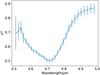 |
Fig. 10 Observed squared visibilities as a function of wavelength near the 4.7 μm dip. The data for all baselines were averaged. |
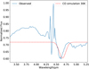 |
Fig. 11 Observed LM-band spectrum (solid line) is compared to a simple simulation (dashed line) of absorption at the CO fundamental band near 4.6 μm and at a gas temperature of 30 K. The simulated spectrum was smoothed to the spectral resolution of MATISSE. |
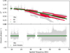 |
Fig. 12 K band squared visibilities and closure phases measured with GRAVITY (gray). Best-fit geometrical models for elliptical disk (ED) and circular disk (CD), are also shown, with both having zero closure phases. |
3.4 K-band geometrical modelling (GRAVITY and MYSTIC)
The GRAVITY K band observations for V838 Mon are the most extensive of all the VLTI observations that we have obtained so far. Observations on all three array configurations (including the intermediate configurations) were successfully executed, which resulted in good sampling of the UV plane. This allowed us to perform the subsequent image reconstruction (see Sect. 4.2). We obtained 15 out of the requested 18 observing runs. Results are shown in Fig. 12. The source is well resolved at the longest baselines, as the squared visibilities fall to a minimum of 0.1. Some of the baselines of the extended configuration reveal smaller peak-like features in the squared visibilities, which cannot be explained by just a simple disk or a Gaussian model (shown more clearly in Fig. 13). These features arise in the observations taken with the baselines J2-A0 and J3-A0, and can be seen in Figs. G.11 and G.12. The squared visibilities do not change considerably with wavelength over most of the wavelength range, except at regions dominated by the water spectral feature (at 2 μm) and the CO overtones (2.3–2.4 μm), as seen in Figs. 14 and 15). This is why we also obtained size estimates for the CO and water emitting regions as well by restricting ourselves to those particular wavelength ranges. This suggests that the shape of the structure is mostly independent of wavelength in the K band. This can be seen in the figures shown in Appendix G, where any rise and fall in the visibilities is minor (~0.1). The closure phases seem to scatter around zero by a few degrees and reach a maximum of ~5°, with a mean error of ~0.5°. Once again, like the squared visibilities they too do not seem to vary drastically as seen in the figures presented in Appendix H. The root-mean-square (RMS) scatter is 2° which suggests that the observed deviations in the closure phases can be attributed mostly to observational noise (within 4σ) and maybe some very small asymmetries present in V838 Mon.
Although the K-band data were used extensively for imaging, we nevertheless thought it prudent to also model the visibilities directly using simple geometrical models in order to obtain constraints on the size of the structure. The best-fit parameters for all models are shown in Table A.1. The size of the source lies in the range 1.2–2.6 mas, depending on the choice of model. The value of the PA in the K band is similar to measurements in the other bands.
We were also able to obtain K band spectra with a medium resolution (R ~ 500). The spectrum was calibrated using the star HD 54990. This resulted in the removal of the major telluric feature caused by H2O near 2 μm, leaving us with absorption bands in the range 2.3–2.35 μm and less intense absorption features near 2 μm. We identified these as CO and H2O features, respectively. To ensure that this identification was accurate, we modelled the absorption at various temperatures using pgopher (Western 2017) and spectroscopic data from the EXOMOL database (Tennyson et al. 2020). The models represent a simple slab of gas in local thermodynamic equilibrium (i.e. characterized by a single temperature) and optically thin absorption. Observed spectra are compared to the simple simulations in Figs. 14–16. After experimenting with a wide range of temperatures for both species, we find that a model with a CO temperature of 3000 K and an H2O temperature of 1000 K best represents the data, however, due to the poor spectral resolution, these are only very rough constraints. The absorption may arise in the photosphere or very close to it in the circumstellar gas (cf. Geballe et al. 2007). We use geometrical modelling to determine the sizes of the source when the visibilities are limited to spectral regions where molecular absorption is strongest. For CO, we restrict the GRAVITY data to 2.29-2.37 μm, whereas for water 1.97–2.07 μm was selected. By fitting circular disk models to each of these datasets, we obtained angular diameters of 2.1 ± 0.1 mas and 2.0 ± 0.1 mas, respectively. With the uncertainties, these results are consistent with the size obtained for the entire band.
We also obtained a single night of MYSTIC K band observations and geometrically modelled the visibilities with a uniform disk and an elliptical disk model. The results are shown in Fig. 17. The uniform disk model yields an angular diameter of 1.57 ± 0.01, mas while the elliptical disk model yields an angular diameter of 1.72 ± 0.01 mas, PA of −41.6 ± 1.5°, and a stretch ratio of 1.28 ± 0.01. Due to the longer CHARA baselines, V838 Mon is much better resolved, as evidenced by the lower minimum squared visibility. Additionally, we also combined both the GRAVITY and MYSTIC K band squared visibilities and performed a uniform disk fit to the resulting combined dataset, which gave an angular diameter of 1.94 ± 0.01 mas. This value is essentially the same as the one obtained from fitting only the GRAVITY squared visibilities, which suggests that combining them with the MYSTIC squared visibilities does not result in a significant change in the size estimate for V838 Mon.
The mean of the MYSTIC closure phases is ~2° with an RMS of ~11°, which strongly hints towards the presence of asymmetries. Unlike the GRAVITY dataset, the MYSTIC observations lasted only a single night because of which we could only geometrically model the closure phases. The results of this modelling are presented in Sect. 4.5.
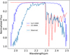 |
Fig. 14 Synthetic spectra generated for H2O at 1000 K and for CO at 3000 K are compared to the observed K band spectrum from GRAVITY over the entire observed band. The synthetic spectra are arbitrary scaled. The simulation does not include high-opacity effects, which may result in the poor fit to the observed saturated water band near 2 μm. The synthetic spectra were convolved to the spectral resolution of the GRAVITY resolution. |
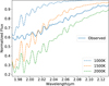 |
Fig. 15 Synthetic spectra of water generated at various temperatures are compared to the observed spectrum (blue). |
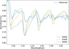 |
Fig. 16 Synthetic spectra generated for the first-overtone CO bands at various temperatures. The solid blue line is the observed spectrum. |
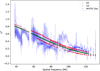 |
Fig. 17 K-band squared visibilities as measured with MYSTIC (blue). Best-fit geometrical models for elliptical disk (ED) and circular disk (CD) are also shown. |
3.5 H-band geometrical modelling
CHARA MIRC-X observations allowed us to observe V838 Mon in the H band as well. Previous measurements in the H band were taken in 2012 using the AMBER instrument and prior to that, in 2004 (Lane et al. 2005) with the Palomar Testbed Interferometer (PTI). These recent CHARA measurements serve as a direct follow-up to the previous H band observations. The squared visibilities, shown in Fig. 18, suggest that the source is resolved at the longest CHARA baselines (≲331 m), as the visibilities fall to a minimum of 0.1. The mean uncertainity is ~4°. The closure phases split into two groups. One is scattered around null phase, and the other, more populous group, is centered at phases ~6°, thereby hinting towards deviations from centro-symmetry in some parts of the remnant. This pattern is observed at all spatial frequencies and requires a more complex source structure, which we discuss in Sect. 4.3.
4 Image reconstruction
4.1 L band image reconstruction
For the purposes of the image reconstruction, we combined the 2021/2022 MATISSE L-band data set with the one from 2020 used by Mobeen et al. (2021), since no significant variability occurred in the source over the course of the year. This is further confirmed by our modelling of the recent visibilities and phases presented in Sect. 3.1. Because both of the datasets consist of observations made with the large configuration, any reconstructed image will be sensitive to compact features in V838 Mon. The image was constructed using the image reconstruction algorithm Multi-aperture Image Reconstruction Algorithm MIRA (Thiébaut 2008) which uses a likelihood cost-function minimization method. For the L-band image, we set a pixel size of 0.1 mas, which is significantly smaller (~30 times) than the theoretical best resolution achievable with VLTI at this wavelength (λL/2Bmax ≈ 3 mas). This pixel size was chosen so that the image plane could be adequately filled, since the size of V838 Mon in the L band is on the order of the best resolution attainable (~3 mas). Also, we used a similar pixel size in Mobeen et al. (2021) when we attempted to construct an image using the few MATISSE observations obtained in 2020. A FoV of 5 mas was chosen, taking into consideration the size of the L band structure inferred from geometrical modelling (see Table A.1).The regularization scheme we employed was the hyperbolic regularization with a regularization parameter of 106. These regularization settings resulted in images with the lowest χ2 values.
The resulting image displayed in Fig. 19 shows an asymmetrical, elliptical feature. The geometric orientation is along the PA that we obtained from our modelling presented in the prior sections.
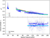 |
Fig. 18 Observations (dark blue) and best fit models for the H band squared visibilities and closure phases. Circular (CD) and elliptical (ED) disk models are shown. |
4.2 K-band image reconstructions
Given the comprehensive nature of our GRAVITY observations, we were able to perform detailed image reconstruction of V838 Mon from the measured interferometric observables in the K band. For this purpose, we used two separate image reconstruction algorithms: SQUEEZE (Baron et al. 2010) and MIRA (Thiébaut 2008). Both these algorithms attempt to solve for the best image given the data and a model of the image. They employ different methodologies and minimization techniques from one another. Thus, by using multiple algorithms to reconstruct an image and comparing them to one another, one can distinguish between authentic features present in a source and artefacts that could have resulted from the different algorithms. The best resolution (λL/2Bmax) attainable with VLTI baselines in the K band is ~ 2 mas. For the purpose of our image reconstruction, we limited our FoV to 10 mas and set the pixel size to 0.1 mas, making the image 100 by 100 pixels. This choice for the FoV and pixel size was adopted after taking into consideration the size of V838 Mon as inferred from geometrical modelling (~ 2 mas). With MIRA, just as in the L band, we used the hyperbolic regularization and found that the χ2 was minimized with a regularization parameter of 106. However, with the SQUEEZE algorithm, we used the total variation and found the χ2 to be minimized with a parameter value of 103. Total variation with a high enough regularization parameter value is identical to the hyperbolic regularization scheme. The values for the regularization parameters were determined by reconstructing images for a wide range of parameter values and by noting the value at which no further reduction in χ2 takes place. This parameter is significant since it sets the weight for the image model against the data when the minimization scheme is implemented. We combined all the GRAVITY OIFITS files and merged them into a single file by using OI-Tools8. This yielded a single OIFITS file that was then used as the input file in the image algorithms. The number of iterations was set at 500. Finally, a randomly generated image was used as the starting image for all of our reconstruction attempts. The reconstruction results with both MIRA and SQUEEZE are shown in Figs. 20 and 21, respectively. We performed image reconstruction using a different strategy as well, whereby the combined GRAVITY data OIFITS file was binned into smaller wavelength increments of 0.05 μm. The image in the first wavelength bin in this process was constructed with a random starting image. However, in subsequent reconstructions for the other bins, the starting image used would be the image obtained for the preceding bin. Using this chain imaging method helped us to significantly decrease the value of the reduced χ2, namely: from ≈150 to ≈ 8 in the final image. Thus, the final image is at the endpoint of the waveband. The result of this strategy is displayed in Fig.22.
The resulting images (Figs. 20 and 21) from both algorithms display a similar morphology in the K band. In the 0.1 mas image reconstructions, multiple possible features are immediately noticeable. These include the clump-like features (labelled as A, B, D, E, and G in Fig. 20) that are roughly distributed along an axis at the PA value (~−40°) which we have obtained from geometrical modelling and which is similar to the PA found for the disk-like feature found in V838 Mon in other bands. Furthermore, we also see two narrow linear features (labelled C and F in Fig. 20) stretching along the northeast direction, which appear to be nearly perpendicular to the axis defining the brighter clumps. When we look at the reconstructed image made using SQUEEZE, we see that despite being generally similar to its MIRA counterpart, the structure in the SQUEEZE image is a lot more continuous and somewhat resembles a clumpy disjointed ring seen at an intermediate inclination. The features that correspond to regions A, B, D, E, and G in Fig. 20, are present in Fig. 21; however, features C and F are not clearly distinguishable in the SQUEEZE image. This could mean that the linear features are imaging artefacts.
Our highest resolution (0.1 mas) K-band images reveal a very clumpy morphology that surrounds the central elliptical structure (see Fig. 20). The major clumps seem to almost trace out a ring that has a size of about 5 mas, while the inner source spans 2 mas. It is worth noting that at the adopted pixel size of 0.1 mas, the source is already super-resolved when compared to the actual achievable resolution with the longest baseline at the VLTI (i.e. ~2 mas). Thus, the finer details such as the clumps and linear features could be simply image artefacts that arise as a consequence of using too high a resolution. To further explore the effects of super-resolution, we performed image reconstruction using larger pixel sizes of 0.5 and 0.8 mas. These results can be seen in Figs. A.1–A.4. The resulting less super-resolved images show only a single extended feature, whereas the inner feature seen in the more resolved images ceases to be distinguishable. Furthermore, the clumps that were prominent in the 0.1 mas resolution image also seem to have vanished; however, the extended structure in the 0.5 mas and 0.8 mas images seems to suggest that the circumstellar environment is asymmetrical and exhibits a morphology that could be described as bipolar. The orientation of this bipolar structure is along the same axis defined by the PA from the geometrical model fitting. It is likely that the outer structure is indeed an example of outflows that are expected to be produced in post-merger environments, similar to what is seen in the sub-mm regime in the stellar merger remnant V4332 Sgr (Kamiński et al. 2018).
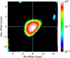 |
Fig. 19 Image reconstruction of V838 Mon done in the L band using the combined 2020–2022 MATISSE data. Flux is in a logarithmic scale in arbitrary units. The nominal resolution is 3 mas and χ2 ~ 4. |
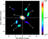 |
Fig. 20 Reconstructed K band image of V838 Mon obtained using the MIRA imaging algorithm. Flux level is logarithmic, and the units are arbitrary. Nominal resolution is 2 mas and χ2 ~150. |
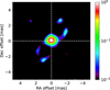 |
Fig. 21 Reconstructed K band image of V838 Mon obtained using the SQUEEZE imaging algorithm. Nominal resolution is 2 mas and χ2 ~150. |
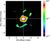 |
Fig. 22 Reconstructed K band image of V838 Mon obtained using the chain imaging method with the MIRA imaging algorithm. Nominal resolution is 2 mas and χ2 ~ 8. |
4.3 H band image reconstruction
Adopting an approach that is similar to the one we used to analyze the K-band data, we employed the same imaging algorithms and attempted image reconstruction for the CHARA observations in the H band. With CHARA, given its longer baselines (maximum baseline of ~300 m), the best attainable resolution is about 0.5 mas. The image FoV was set to 10 mas, while a pixel size of 0.1 mas was chosen and the starting image was randomly generated. The value of the regularization was set to 1000 for both MIRA and SQUEEZE imaging. The resulting images (Figs. 23 and 24) show an elongated structure that is oriented at a PA of −40°. The physical extent of this feature is about 2 mas, thus allowing us to probe the innermost parts of the circumstel-lar environment. Despite the fact that the images provide a very good fit to the data (i.e. reduced χ2 = 1) some artefacts are also present. We define artefacts as low intensity features (contrast ratio less than equal to 0.01), that are unique to a particular image reconstruction algorithm. These might have occurred due to the fact that we were only able to use 4–5 telescopes on any given night and not the full six telescope configuration of CHARA.
It would seem that in the H band we are also seeing a similar bipolar feature, but at much smaller spatial scales, placing it closer to the central merger remnant. The reconstructed images in the H band show a structure that is similar in morphology to its counterparts in other wavelength regimes. The images indicate the presence of asymmetrical structures in the south-east and north-west regions of V838 Mon. The asymmetry is most noticeable in the northern part of the bipolar structure, which seems to be misaligned with respect to the southern feature. A crucial difference in the H band structure is the relatively high closure phase deviations and the apparent asymmetrical shape of the northern lobe visible in the image reconstructions. The orientation of the CHARA feature is in good agreement with what is seen in the L, M, and K bands. This can be seen in the sketch of the NIR-MIR structures in Fig. 6.
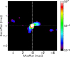 |
Fig. 23 Reconstructed H band image of V838 Mon obtained using the MIRA imaging algorithm. The nominal resolution is 0.5 mas and χ2 ~ 1. |
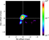 |
Fig. 24 Reconstructed H band image of V838 Mon obtained using the SQUEEZE imaging algorithm. The nominal resolution is 0.5 mas and χ2 ~ 1. |
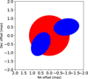 |
Fig. 25 Model we used for explaining the H-band closure phases. The red central component represents the star, while the blue ellipses may represent bipolar outflows hinted by the H band image reconstructions (cf. Figs. 23 and 24). About 95% of the model flux is contained within the central component. |
4.4 H-band closure phase modelling
As mentioned previously, we were unable to explain H band closure phases with simple geometrical models (circular and elliptical disks, see Sect. 3.5). Given the magnitude of these closure phase deviations, it is apparent that the circumstellar structure in V838 Mon possesses significant asymmetries. This is further corroborated by our imaging results presented in Sect. 4.3. Similarly to the K-band images, the H-band ones seem to show a bipolar structure which is roughly oriented along the same PA as all the other structures that encase the merger remnant. Given our imaging results in the H band, we again attempted to reproduce the closure phase deviations, this time using a more complicated multi-component model that better represents the structure as revealed by the H band image. A sketch of this model is shown in Fig. 25. The model includes a central 1 mas disk that represents the central star. In addition to that, we also include two elliptical disks (‘clumps’). The semimajor axis of the lower ellipse is oriented roughly along the PA that the structures in other bands follow, while that of the upper ellipse is nearly horizontal. The modelled and observed closure phases are plotted as a function of spatial frequency in Fig. 26. We see that the more complex model inspired by the image reconstructions is able to explain the closure phase deviations quite satisfactorily. Additionally, we tried a model comprising a uniform disk and two point sources, but the resulting closure phase deviations from that model were too high, by a factor of almost 10, which is why we discarded it.
4.5 MYSTIC K band closure phase modelling
As stated earlier in this work, the K band closure phases as observed by MYSTIC do show significant non-zero deviations. Therefore, we decided to model these closure phases geometrically to see if the observations can be well explained with an asymmetric intensity distribution. We used the interferometric modelling software PMOIRED (Mérand 2022) for this purpose. Using PMOIRED, we experimented with various combinations of geometrical building blocks (disks, Gaussians, etc.) in order to reproduce the closure phases as accurately as possible. Ultimately, we found the best-fit model (χ2 ~ 1.5), consisting of an elongated primary disk with a size of 1 mas and a smaller (0.5 mas), less intense secondary disk that is separated from the primary by ~ 1.7 mas. The sizes of the primary and secondary components were fixed at 1 and 0.5 mas, respectively, while the orientation and elongation of the primary component were fixed at −40° and 1.4. The primary component was fixed in the center of the FoV, and its flux level was set at 90%, while the secondary flux level was set at 10%. The x and y positions of the secondary were left as free parameters. The geometry of this model can be seen in Fig. 27.
The closure phases produced by the model and their fit to the observations are shown in Fig. 28. We can see from the figure that the non-zero closure phases are explained quite satisfactorily by our model at all baselines. The orientation of the primary disk seems to agree well with the general orientation of V838 Mon, as seen in the HK band image reconstructions. Furthermore, the PA of the smaller disk component with respect to the primary also closely resembles the general orientation of V838 Mon in the NIR-MIR bands. The modelling results prove that the closure phase deviations are well explained with the addition of an off-centre ‘clump’.
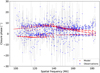 |
Fig. 26 Simulated and observed H-band closure phases as a function of spatial frequency. The simulated closure phases are represented by red triangles, while the observations are represented by the blue circles. Simulations correspond to the structure shown in Fig. 25 and match the observations better than the simpler models described in Sect. 3.5. |
5 Discussion
5.1 Jets
Lane et al. (2005) suggested that V838 Mon could potentially possess an asymmetric structure, however, due to their limited observations and absence of closure phase measurements they were unable to prove this conclusively. In Mobeen et al. (2021), the L band closure phases seemed to be hinting towards minor asymmetries, as indicated by the small but non-zero deviations. However, we interpreted them with great caution given their small magnitude and the limited data. In this study, we have conclusively shown the existence of these asymmetries via geometrical modelling and image reconstruction in the HK bands.
The GRAVITY and CHARA images (see Figs. 20 and 23) show an inhomogeneous bipolar structure. This inhomogeneous structure is more pronounced in the H band image, as we can see that the northern lobe is oriented at a different PA than its southern counterpart. The asymmetric lobes model is further corroborated by H band closure phases that are satisfactorily explained when we assume such a morphology for our geometrical model (see Figs. 25 and 26).
These outflows resemble jets, which are strongly believed to be present in intermediate-luminosity optical transients (ILOTs), such as luminous red novae (LRNs) and are thought to play an important role by providing the extra energy needed to unbind the common envelope. Soker (2016) showed that energy from the jets is transferred to the primary envelope during the grazing envelope evolution stage, which means that the jets could be the mechanism responsible for the outbursts seen in LRNs, including V838 Mon. In a subsequent study (Soker 2020) it was shown that the luminosity and total energy output of V838 Mon could be adequately explained if jets present in the system collide with a slow-moving shell of material. The author concluded that this was a plausible scenario for V838 Mon and V4332 Sgr. In the case of V4332 Sgr, it was shown using submillimeter observations carried out at ALMA (Kamiński et al. 2018) that the object does indeed possess bipolar outflows consisting of molecular material. This means that jets were a main component in the LRN event in V4332 Sgr. If jets are the reason for the LRN in V838 Mon, this would mean that we should be able to observe jet-like features in the source. Since we see a clear bipolar structure in the image reconstructions for V838 Mon (see Sects. 4.2 and 4.3) this means that jets played a role in the energy output of the outburst in 2002 which resulted in V838 Mon brightening by several orders of magnitude. Soker (2023) shows that only jets can satisfactorily explain the rapid rise in luminosity that is seen in ILOTS such as V838 Mon and V1309 Sco just prior to the outbursts. As of now, no jets have been observed in V1309 Sco, but the clear detection of jets in V838 Mon, V4332 Sgr and CK Vulpeculae suggests that such bipolar features are perhaps universal amongst many other stellar merger remnants. Recently, the Blue Ring Nebula was found to possess bipolar conical outflows which led Hoadley et al. (2020) to conclude that the object is a result of a stellar merger. Our interferometric observations of V838 Mon appear to be lending credence to the idea that jets are an intrinsic feature of LRNs and persist even in the post-merger environment.
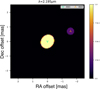 |
Fig. 27 Image for the best-fit geometric model comprising two components in the K band. The primary component is the elliptical disk with a size of ~ 1 mas and elongated at a PA of −40°. The secondary component is a smaller circular disk with a diameter of 0.5 mas and separated from the primary by ~1.7 mas. The model flux contained in the secondary component is ~10%. |
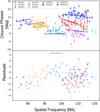 |
Fig. 28 MYSTIC K-band closure phases (top) for the observed (points) and modelled (lines) visibilities representing the model in Fig. 27. The bottom panel shows the respective residuals. |
5.2 Clumps
The MYSTIC closure phases, as evidenced by the modelling, suggest the presence of a small clump separated from the central star by ~1.7 mas. The clump lies approximately along the PA traced by the bipolar structure in V838 Mon; in fact, its orientation seems to be quite similar to that of the northern lobe seen in the H band. This clump is the first ever detection of a sub milliarcsecond feature in V838 Mon. The exact nature of the clump (whether stable or transient) remains elusive. ALMA maps of V838 Mon by Kamiński et al. (2021) also showed the presence of prominent clumps in the wind component of the merger remnant in the submillimeter regime. The formation of dust clumps is a prevalent phenomenon amongst red supergiants (RSGs) and asymptotic giant branch stars. VX Sagittarii, which is a variable supergiant star, has been found to possess an inhomogeneous atmosphere containing spots (Chiavassa et al. 2010). Using radiative hydrodynamical simulations Chiavassa et al. (2009) showed that the interferometric observations for the RSG α Ori could be explained using limb darkening models, which suggested the presence of asymmetric surface features. In addition to this, Kamiński (2019) showed using ALMA observations that multiple dust clumps had formed in the RSG VY Canis Majoris (VY CMa). A dust clump is also thought to have formed in the (RSG) Betelgeuse during the Great Dimming event of 2019–2020 (Montargès et al. 2021). Follow-up VLTI/MATISSE observations in 2020 were obtained by Cannon et al. (2023) which showed a complex closure phase signal in Betelgeuse. The authors constructed multiple radiative transfer models, such as those consisting of clumps and spots. Although they could not reproduce the closure phase signal exactly due to their use of only rudimentary models, the authors concluded that either clumps or other surface features were the main source of the closure phase deviations. In the case of V838 Mon, the closure phases are not as high as those in Betelgeuse observed by Cannon et al. (2023); however, as shown in Sect. 4.5, the MYSTIC closure phases can only be explained by the smaller clump (see Fig. 27).
Since the spectra for V838 Mon resembles that of a late M-type supergiant (Evans et al. 2003; Loebman et al. 2015), we expect the circumstellar environment in V838 Mon to be somewhat similar to other evolved stars with clumpy surroundings. This particular clump that we have been able to constrain with MYSTIC could in fact be a smaller feature within the lobe- or jetlike structure that is observed at longer wavelengths. This would mean that the lobes themselves could be clumpy and inhomo-geneous. These clumps could be the result of the jet interacting with the surrounding less dense material in the V838 Mon during its common envelope phase. Soker (2019) proposed that this interaction between the jet and the envelope results in the formation of jet-inflated low-density bubbles. As a consequence, the surrounding medium is prone to clumping due to Rayleigh-Taylor instabilities. This would result in the jet departing from a pure axisymmetric morphology and become variable in direction and brightness. It could be the case that the observed H band clump was the result of such jet-inflated bubbles.
5.3 Polarization in V838 Mon
The Gemini speckle image reconstructions in the V and I band speckle images show a morphology that is consistent with the interferometric imaging and modelling results in the HKLMN bands. Both images (see Figs. 4 and 5) seem to suggest that the innermost vicinity in V838 Mon is quite noticeably bright at 562 nm and 832 nm. If this emission results from scattered light, then it is likely to produce a net polarization. It was shown by Wisniewski et al. (2003b) that a low degree of polarization (1%) was present in 2003 in the V band, with a measured PA of 150°. The authors suggested that this polarization signal was pointing to asymmetries in the surroundings of V838 Mon. A follow-up measurement (six months later) showed that the PA of the polarization vector flipped by 90° (Wisniewski et al. 2003a). This change over the course of six months seemed to suggest the dynamic, evolving nature of the dusty environment in V838 Mon. The Gemini observations reveal a complex circumstellar medium in V838 Mon that might still be dynamic and could show signs of varying intrinsic polarization and PA, especially in the V band. The above-mentioned observations by Wisniewski et al. (2003b) and Wisniewski et al. (2003a) were carried out over two decades ago, and since the dramatic change in PA occurred over a period of only six months, we expect the environment in V838 Mon to have significantly changed since then. Future polarimetric measurements could help to determine if linear polarization in V838 Mon has increased significantly over the last two decades.
6 Conclusions
In this study, we performed a multi-wavelength interferometric analysis of the stellar merger remnant V838 Mon in the HKLM bands using the VLTI instruments MATISSE and GRAVITY, as well as the CHARA instrument MIRC-X/MYSTIC. In the HK bands, we imaged the circumstellar environment in the immediate vicinity of the central merger remnant; while in the other bands, we resorted to geometrical modelling to obtain constraints on the geometry and orientation of the post-merger environment. We were also able to compare the HKLMN image reconstructions with I and V band speckle imaging from Gemini South. In addition, we modelled the spectral features that were present in the K and M bands and we were able to put constrains on the temperatures. Our main findings are as follows.
Geometrical modelling suggests that the L band structure has remained largely the same since previous observations presented in Mobeen et al. (2021).
Image reconstruction in the HK bands reveals a bipolar morphology that resembles jets. These ‘jets’ are present in both bands, while in the H band they appear to be slightly asymmetric as well.
The super resolved GRAVITY K band images reconstructed with a 0.1 mas pixel size reveal clumpy outflows that surround the inner feature.
The MYSTIC K band closure phases are aptly explained by a small (0.5 mas), off-centre circular feature that we identify as a potential clump.
The orientation of the extended circumstellar feature (i.e. outflows) tends to be along the same general direction namely, north-west, with a PA that varies from −30° to −50° and an ellipticity in the range 1.1–1.6, depending on the wavelength. This is in agreement with prior studies (Chesneau et al. 2014; Kamiński et al. 2021). However, the N– and I–band structure is oriented along the north-south direction.
The K band CO and water features are best modelled at temperatures of 2000–3000 K, thereby hinting at their pho-tospheric origin. We were also able to measure the sizes of the CO and water emitting regions, namely: 2.1 mas and 1.985 mas, respectively. In the M band, we observe CO at 4.6 μm, for the first time, using interferometry.
Acknowledgements
T.K. and M.Z.M. acknowledge funding from grant no 2018/30/E/ST9/00398 from the Polish National Science Center. Based on observations made with ESO telescopes at Paranal observatory under program IDs 0104.D-0101(C) and 0108.D-0628(D). This research has benefited from the help of SUV, the VLTI user support service of the Jean-Marie Mariotti Center (http://www.jmmc.fr/suv.htm). This research has also made use of the JMMC’s Searchcal, LITpro, OIFitsExplorer and Aspro services available at http://www.jmmc.fr/. This research has made use of the Jean-Marie Mariotti Center JSDC catalogue available at http://www.jmmc.fr/catalogue_jsdc.htm. This work is based upon observations obtained with the Georgia State University Center for High Angular Resolution Astronomy Array at Mount Wilson Observatory. The CHARA Array is supported by the National Science Foundation under Grant No. AST-1636624 and AST-2034336. Institutional support has been provided from the GSU College of Arts and Sciences and the GSU Office of the Vice President for Research and Economic Development. Time at the CHARA Array was granted through the NOIRLab community access program (NOIRLab PropID: 2022A-426176; PI: M. Mobeen). SK acknowledges funding for MIRC-X from the European Research Council (ERC) under the European Union’s Horizon 2020 research and innovation programme (Starting Grant No. 639889 and Consolidated Grant No. 101003096). JDM acknowledges funding for the development of MIRC-X (NASA-XRP NNX16AD43G, NSF-AST 1909165) and MYSTIC (NSF-ATI 1506540, NSF-AST 1909165). Some of the observations in this paper made use of the High-Resolution Imaging instrument Zorro and were obtained under Gemini LLP Proposal Number: GN/S-2021A-LP-105. Zorro was funded by the NASA Exoplanet Exploration Program and built at the NASA Ames Research Center by Steve B. Howell, Nic Scott, Elliott P. Horch, and Emmett Quigley. Zorro was mounted on the Gemini South telescope of the international Gemini Observatory, a program of NSF’s OIR Lab, which is managed by the Association of Universities for Research in Astronomy (AURA) under a cooperative agreement with the National Science Foundation. on behalf of the Gemini partnership: the National Science Foundation (United States), National Research Council (Canada), Agencia Nacional de Investigacion y Desarrollo (Chile), Ministerio de Ciencia, Tecnologia e Innovacion (Argentina), Min-istério da Ciência, Tecnologia, Inovaçôes e Comunicaçôes (Brazil), and Korea Astronomy and Space Science Institute (Republic of Korea).
Appendix A Images at lower resolutions
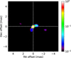 |
Fig. A.1 H band image for V838 Mon with MIRA algorithm at a resolution of 0.2 mas. The nominal resolution is 0.5 mas . χ2 ~1 |
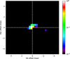 |
Fig. A.2 H band image for V838 Mon with MIRA algorithm at a resolution of 0.5 mas. The nominal resolution is 0.5 mas |
. χ2 ~1
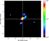 |
Fig. A.3 K band image for V838 Mon with MIRA algorithm at a resolution of 0.5 mas. The nominal resolution is 2 mas. χ2 ~150 |
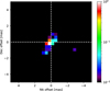 |
Fig. A.4 K band image for V838 Mon with MIRA algorithm at a resolution of 0.8 mas. The nominal resolution is 2 mas. χ2 ~150 |
Fitted models and their parameters.
Appendix B Observables as functions of wavelength in the LM bands
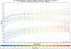 |
Fig. B.1 Squared visibilities versus wavelength in the L band for the nights 30 October 2021, 2 March 2022, and 30 March 2022. The colour bar represents the wavelength. |
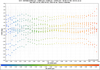 |
Fig. B.2 Closure phases versus wavelength in the L band for the nights 30 October 2021, 2 March 2022, and 30 March 2022. The colour bar represents the wavelength. |
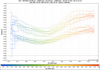 |
Fig. B.3 Squared visibilities versus wavelength in the M band for the nights 30 October 2021, 2 March 2022, and 31 March 2022. The colour bar represents the wavelength. |
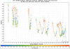 |
Fig. B.4 Squared visibilities versus spatial frequency in the M band for the nights 30 October 2021, 2 March 2022, and 31 March 2022. The colour bar represents the wavelength. |
Appendix C Κ band imaging V2 residuals
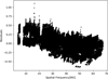 |
Fig. C.1 Residuals for the synthetic squared visibilities derived from the 0.1 mas GRAVITY reconstructed image. |
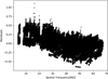 |
Fig. C.2 Residuals for the synthetic squared visibilities derived from the 0.5 mas GRAVITY reconstructed image. |
 |
Fig. C.3 Residuals for the synthetic squared visibilities derived from the 0.8 mas GRAVITY reconstructed image. |
Appendix D Κ band imaging closure phase residuals
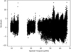 |
Fig. D.1 Residuals for the synthetic closure phases derived from the 0.1 mas GRAVITY reconstructed image. |
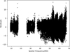 |
Fig. D.2 Residuals for the synthetic closure phases derived from the 0.5 mas GRAVITY reconstructed image. |
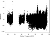 |
Fig. D.3 Residuals for the synthetic closure phases derived from the 0.8 mas GRAVITY reconstructed image. |
Appendix E H band imaging V2 residuals
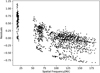 |
Fig. E.1 Residuals for the synthetic squared visibilities derived from the 0.1 mas CHARA reconstructed image. |
 |
Fig. E.2 Residuals for the synthetic squared visibilities derived from the 0.2 mas CHARA reconstructed image. |
 |
Fig. E.3 Residuals for the synthetic squared visibilities derived from the 0.5 mas CHARA reconstructed image. |
Appendix F H band imaging closure phase residuals
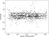 |
Fig. F.1 Residuals for the synthetic closure phases derived from the 0.1 mas CHARA reconstructed image. |
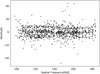 |
Fig. F.2 Residuals for the synthetic closure phases derived from the 0.2 mas CHARA reconstructed image. |
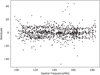 |
Fig. F.3 Residuals for the synthetic closure phases derived from the 0.5 mas CHARA reconstructed image. |
Appendix G Κ band squared visibilities
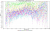 |
Fig. G.1 Squared visibilities versus wavelength in the Κ band for the night 3 February 2022. |
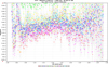 |
Fig. G.2 Squared visibilities versus wavelength in the Κ band for the night 3 February 2022. |
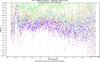 |
Fig. G.3 Squared visibilities versus wavelength in the Κ band for the night 4 February 2022. |
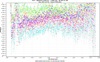 |
Fig. G.4 Squared visibilities versus wavelength in the Κ band for the night 4 February 2022. |
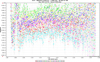 |
Fig. G.5 Squared visibilities versus wavelength in the Κ band for the night 4 February 2022. |
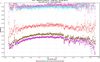 |
Fig. G.6 Squared visibilities versus wavelength in the Κ band for the night 11 March 2022. |
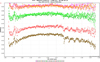 |
Fig. G.7 Squared visibilities versus wavelength in the Κ band for the night 5 February 2022. |
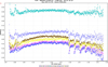 |
Fig. G.8 Squared visibilities versus wavelength in the Κ band for the night 4 January 2022. |
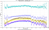 |
Fig. G.9 Squared visibilities versus wavelength in the Κ band for the night 11 February 2022 |
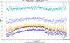 |
Fig. G.10 Squared visibilities versus wavelength in the Κ band for the night 13 February 2022. |
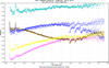 |
Fig. G.11 Squared visibilities versus wavelength in the Κ band for the night 25 February 2022. |
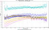 |
Fig. G.12 Squared visibilities versus wavelength in the Κ band for the night 25 February 2022. |
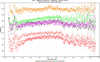 |
Fig. G.13 Squared visibilities versus wavelength in the Κ band for the night 6 February 2022 |
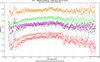 |
Fig. G.14 Squared visibilities versus wavelength in the Κ band for the night 6 February 2022 |
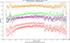 |
Fig. G.15 Squared visibilities versus wavelength in the Κ band for the night 10 February 2022 |
Appendix H K band closure phases
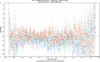 |
Fig. H.1 Closure phases versus wavelength in the Κ band for the night 3 February 2022. |
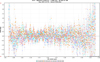 |
Fig. H.2 Closure phases versus wavelength in the Κ band for the night 3 February 2022. |
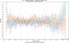 |
Fig. H.3 Closure phases versus wavelength in the Κ band for the night 4 February 2022. |
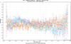 |
Fig. H.4 Closure phases versus wavelength in the Κ band for the night 4 February 2022. |
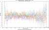 |
Fig. H.5 Closure phases versus wavelength in the Κ band for the night 4 February 2022. |
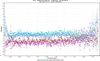 |
Fig. H.6 Closure phases versus wavelength in the Κ band for the night 11 March 2022. |
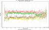 |
Fig. H.7 Closure phases versus wavelength in the Κ band for the night 5 February 2022 |
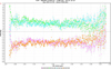 |
Fig. H.8 Closure phases versus wavelength in the Κ band. |
 |
Fig. H.9 Closure phases versus wavelength in the Κ band. |
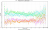 |
Fig. H.10 Closure phases versus wavelength in the Κ band. |
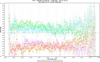 |
Fig. H.11 Closure phases versus wavelength in the Κ band. |
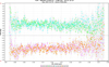 |
Fig. H.12 Closure phases versus wavelength in the Κ band. |
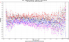 |
Fig. H.13 Closure phases versus wavelength in the Κ band. |
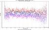 |
Fig. H.14 Closure phases versus wavelength in the Κ band. |
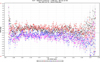 |
Fig. H.15 Closure phases versus wavelength in the Κ band. |
References
- Anugu, N., Le Bouquin, J.-B., Monnier, J. D., et al. 2020, AJ, 160, 158 [NASA ADS] [CrossRef] [Google Scholar]
- Banerjee, D. P. K., & Ashok, N. M. 2002, A&A, 395, 161 [NASA ADS] [CrossRef] [EDP Sciences] [Google Scholar]
- Banerjee, D. P. K., Varricatt, W. P., & Ashok, N. M. 2004, ApJ, 615, L53 [NASA ADS] [CrossRef] [Google Scholar]
- Baron, F., Monnier, J. D., & Kloppenborg, B. 2010, SPIE Conf. Ser., 7734, 77342I [Google Scholar]
- Bond, H. E., Henden, A., Levay, Z. G., et al. 2003, Nature, 422, 405 [CrossRef] [Google Scholar]
- Bourgés, L., Lafrasse, S., Mella, G., et al. 2014, ASP Conf. Ser., 485, 223 [NASA ADS] [Google Scholar]
- Bourgés, L., Mella, G., Lafrasse, S., et al. 2017, VizieR Online Data Catalog: II/346 [Google Scholar]
- Cannon, E., Montargès, M., de Koter, A., et al. 2023, A&A, 675, A46 [NASA ADS] [CrossRef] [EDP Sciences] [Google Scholar]
- Chelli, A., Duvert, G., Bourgès, L., et al. 2016, A&A, 589, A112 [NASA ADS] [CrossRef] [EDP Sciences] [Google Scholar]
- Chesneau, O., Millour, F., De Marco, O., et al. 2014, A&A, 569, L3 [NASA ADS] [CrossRef] [EDP Sciences] [Google Scholar]
- Chiavassa, A., Plez, B., Josselin, E., & Freytag, B. 2009, A&A, 506, 1351 [NASA ADS] [CrossRef] [EDP Sciences] [Google Scholar]
- Chiavassa, A., Lacour, S., Millour, F., et al. 2010, A&A, 511, A51 [NASA ADS] [CrossRef] [EDP Sciences] [Google Scholar]
- Cruzalebes, P., Petrov, R. G. P., Robbe-Dubois, S., et al. 2019, VizieR Online Data Catalog: II/361 [Google Scholar]
- Evans, A., Geballe, T. R., Rushton, M. T., et al. 2003, MNRAS, 343, 1054 [CrossRef] [Google Scholar]
- Geballe, T. R., Rushton, M. T., Eyres, S. P. S., et al. 2007, A&A, 467, 269 [NASA ADS] [CrossRef] [EDP Sciences] [Google Scholar]
- GRAVITY Collaboration (Abuter, R., et al.) 2017, A&A, 602, A94 [NASA ADS] [CrossRef] [EDP Sciences] [Google Scholar]
- Hoadley, K., Martin, D. C., Metzger, B. D., et al. 2020, Nature, 587, 387 [NASA ADS] [CrossRef] [Google Scholar]
- Howell, S. B., & Furlan, E. 2022, Front. Astron. Space Sci., 9, 871163 [NASA ADS] [CrossRef] [Google Scholar]
- Howell, S. B., Everett, M. E., Sherry, W., Horch, E., & Ciardi, D. R. 2011, AJ, 142, 19 [Google Scholar]
- Husser, T. O., Wende-von Berg, S., Dreizler, S., et al. 2013, A&A, 553, A6 [NASA ADS] [CrossRef] [EDP Sciences] [Google Scholar]
- Jennison, R. C. 1958, MNRAS, 118, 276 [Google Scholar]
- Kamiński, T. 2019, A&A, 627, A114 [NASA ADS] [CrossRef] [EDP Sciences] [Google Scholar]
- Kamiński, T., Schmidt, M., Tylenda, R., Konacki, M., & Gromadzki, M. 2009, ApJS, 182, 33 [Google Scholar]
- Kamiński, T., Steffen, W., Tylenda, R., et al. 2018, A&A, 617, A129 [NASA ADS] [CrossRef] [EDP Sciences] [Google Scholar]
- Kamiński, T., Tylenda, R., Kiljan, A., et al. 2021, A&A, 655, A32 [NASA ADS] [CrossRef] [EDP Sciences] [Google Scholar]
- Lane, B. F., Retter, A., Thompson, R. R., & Eisner, J. A. 2005, ApJ, 622, L137 [NASA ADS] [CrossRef] [Google Scholar]
- Leinert, C., Graser, U., Przygodda, F., et al. 2003, Ap&SS, 286, 73 [NASA ADS] [CrossRef] [Google Scholar]
- Loebman, S. R., Wisniewski, J. P., Schmidt, S. J., et al. 2015, AJ, 149, 17 [NASA ADS] [CrossRef] [Google Scholar]
- Lopez, B., Lagarde, S., Petrov, R. G., et al. 2022, A&A, 659, A192 [NASA ADS] [CrossRef] [EDP Sciences] [Google Scholar]
- Mérand, A. 2022, SPIE Conf. Ser., 12183, 121831N [Google Scholar]
- Mobeen, M. Z., Kamiński, T., Matter, A., Wittkowski, M., & Paladini, C. 2021, A&A, 655, A100 [NASA ADS] [CrossRef] [EDP Sciences] [Google Scholar]
- Monnier, J. D., Le Bouquin, J.-B., Anugu, N., et al. 2018, SPIE Conf. Ser., 10701, 1070122 [NASA ADS] [Google Scholar]
- Montargès, M., Cannon, E., Lagadec, E., et al. 2021, Nature, 594, 365 [Google Scholar]
- Munari, U., Desidera, S., & Henden, A. 2002a, IAU Circ., 8005, 2 [NASA ADS] [Google Scholar]
- Munari, U., Henden, A., Kiyota, S., et al. 2002b, A&A, 389, L51 [NASA ADS] [CrossRef] [EDP Sciences] [Google Scholar]
- Pastorello, A., Mason, E., Taubenberger, S., et al. 2019, A&A, 630, A75 [NASA ADS] [CrossRef] [EDP Sciences] [Google Scholar]
- Pejcha, O., Metzger, B. D., Tyles, J. G., & Tomida, K. 2017, ApJ, 850, 59 [NASA ADS] [CrossRef] [Google Scholar]
- Petrov, R. G., Malbet, F., Weigelt, G., et al. 2007, A&A, 464, 1 [NASA ADS] [CrossRef] [EDP Sciences] [Google Scholar]
- Scott, N. J., Howell, S. B., Gnilka, C. L., et al. 2021, Front. Astron. Space Sci., 8, 138 [NASA ADS] [CrossRef] [Google Scholar]
- Setterholm, B. R., Monnier, J. D., Le Bouquin, J.-B., et al. 2022, SPIE Conf. Ser., 12183, 121830B [NASA ADS] [Google Scholar]
- Soker, N. 2016, New Astron., 47, 16 [NASA ADS] [CrossRef] [Google Scholar]
- Soker, N. 2019, MNRAS, 483, 5020 [NASA ADS] [CrossRef] [Google Scholar]
- Soker, N. 2020, ApJ, 893, 20 [Google Scholar]
- Soker, N. 2023, Open J. Astrophys., 6, 32 [NASA ADS] [CrossRef] [Google Scholar]
- Sparks, W. B., Bond, H. E., Cracraft, M., et al. 2008, AJ, 135, 605 [NASA ADS] [CrossRef] [Google Scholar]
- ten Brummelaar, T. A., McAlister, H. A., Ridgway, S. T., et al. 2005, ApJ, 628, 453 [Google Scholar]
- Tennyson, J., Yurchenko, S. N., Al-Refaie, A. F., et al. 2020, J. Quant. Spec. Radiat. Transf., 255, 107228 [NASA ADS] [CrossRef] [Google Scholar]
- Thiébaut, E. 2008, SPIE Conf. Ser., 7013, 70131I [Google Scholar]
- Tylenda, R. 2005, A&A, 436, 1009 [NASA ADS] [CrossRef] [EDP Sciences] [Google Scholar]
- Tylenda, R., & Soker, N. 2006, A&A, 451, 223 [NASA ADS] [CrossRef] [EDP Sciences] [Google Scholar]
- Tylenda, R., Kamiński, T., & Schmidt, M. 2009, A&A, 503, 899 [NASA ADS] [CrossRef] [EDP Sciences] [Google Scholar]
- Webbink, R. F. 1976, ApJ, 209, 829 [NASA ADS] [CrossRef] [Google Scholar]
- Western, C. M. 2017, J. Quant. Spectr. Rad. Trans., 186, 222 [Google Scholar]
- Wisniewski, J. P., Bjorkman, K. S., & Magalhães, A. M. 2003a, ApJ, 598, L43 [NASA ADS] [CrossRef] [Google Scholar]
- Wisniewski, J. P., Morrison, N. D., Bjorkman, K. S., et al. 2003b, ApJ, 588, 486 [NASA ADS] [CrossRef] [Google Scholar]
- Wisniewski, J. P., Clampin, M., Bjorkman, K. S., & Barry, R. K. 2008, ApJ, 683, L171 [NASA ADS] [CrossRef] [Google Scholar]
Differential phases were not used, being affected by chromatic effects from the atmosphere that impaired the detection of any meaningful signature; the correction of such chromatic effects is out of the scope of our study.
MDFC is available through VizieR service at https://vizier.u-strasbg.fr/viz-bin/VizieR
For more details on the error calculation in LITpro, see Evolution of LITpro’ by Isabelle Tallon-Bosc; http://www.jmmc.fr/doc/approved/JMMC-PRE-2300-0012.pdf
All Tables
All Figures
|
Fig. 1 UV tracks for MATISSE observing runs in 2021–2022. |
| In the text | |
|
Fig. 2 UV coverage for GRAVITY observing runs. |
| In the text | |
|
Fig. 3 UV coverage for CHARA observing runs in the HK bands. |
| In the text | |
|
Fig. 4 Speckle image reconstruction from March 2022 at 832 nm. A noticeable north-south elongation is visible. The image field of view (FoV) is 0″.85 by 0″.755. North is up, east is left. The lowest reliable emission feature is at 10% of the peak intensity level. |
| In the text | |
|
Fig. 5 Speckle image reconstruction from February 2021 at 562 nm. A prominent north-west elongation is visible. The image FoV is 0″.21 by 0″.14. North is up, east is left. The lowest reliable emission feature is at 10% of the peak intensity level. |
| In the text | |
|
Fig. 6 Sketch of the best fitting elliptical models for V838 Mon in the HKL bands, as observed by MIRC-X, GRAVITY, and MATISSE. |
| In the text | |
|
Fig. 7 Observed (blue) and best fits for the L band squared visibilities and closure phases. The models ED and CD refer to elliptical disk and circular disk, respectively. |
| In the text | |
|
Fig. 8 Observations (blue) and best fit models for the N band visibility amplitudes. The models ED and CD refer to elliptical disk and circular disk, respectively. |
| In the text | |
|
Fig. 9 Observations (blue) and best fit models for the M band squared visibilities and closure phases. Models ED, CD, and 2P refer to elliptical disk, circular disk, and two point sources, respectively. The angular diameters for the CD and ED models are 5.86 ± 0.08 and 4.35 ± 0.09 mas. These size estimates (4–6 mas) most likely represent the dominant circumstellar component. |
| In the text | |
|
Fig. 10 Observed squared visibilities as a function of wavelength near the 4.7 μm dip. The data for all baselines were averaged. |
| In the text | |
|
Fig. 11 Observed LM-band spectrum (solid line) is compared to a simple simulation (dashed line) of absorption at the CO fundamental band near 4.6 μm and at a gas temperature of 30 K. The simulated spectrum was smoothed to the spectral resolution of MATISSE. |
| In the text | |
|
Fig. 12 K band squared visibilities and closure phases measured with GRAVITY (gray). Best-fit geometrical models for elliptical disk (ED) and circular disk (CD), are also shown, with both having zero closure phases. |
| In the text | |
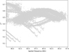 |
Fig. 13 Zoomed-in section on some of the ‘bump’ features in the squared visibilities from Fig. 12. |
| In the text | |
|
Fig. 14 Synthetic spectra generated for H2O at 1000 K and for CO at 3000 K are compared to the observed K band spectrum from GRAVITY over the entire observed band. The synthetic spectra are arbitrary scaled. The simulation does not include high-opacity effects, which may result in the poor fit to the observed saturated water band near 2 μm. The synthetic spectra were convolved to the spectral resolution of the GRAVITY resolution. |
| In the text | |
|
Fig. 15 Synthetic spectra of water generated at various temperatures are compared to the observed spectrum (blue). |
| In the text | |
|
Fig. 16 Synthetic spectra generated for the first-overtone CO bands at various temperatures. The solid blue line is the observed spectrum. |
| In the text | |
|
Fig. 17 K-band squared visibilities as measured with MYSTIC (blue). Best-fit geometrical models for elliptical disk (ED) and circular disk (CD) are also shown. |
| In the text | |
|
Fig. 18 Observations (dark blue) and best fit models for the H band squared visibilities and closure phases. Circular (CD) and elliptical (ED) disk models are shown. |
| In the text | |
|
Fig. 19 Image reconstruction of V838 Mon done in the L band using the combined 2020–2022 MATISSE data. Flux is in a logarithmic scale in arbitrary units. The nominal resolution is 3 mas and χ2 ~ 4. |
| In the text | |
|
Fig. 20 Reconstructed K band image of V838 Mon obtained using the MIRA imaging algorithm. Flux level is logarithmic, and the units are arbitrary. Nominal resolution is 2 mas and χ2 ~150. |
| In the text | |
|
Fig. 21 Reconstructed K band image of V838 Mon obtained using the SQUEEZE imaging algorithm. Nominal resolution is 2 mas and χ2 ~150. |
| In the text | |
|
Fig. 22 Reconstructed K band image of V838 Mon obtained using the chain imaging method with the MIRA imaging algorithm. Nominal resolution is 2 mas and χ2 ~ 8. |
| In the text | |
|
Fig. 23 Reconstructed H band image of V838 Mon obtained using the MIRA imaging algorithm. The nominal resolution is 0.5 mas and χ2 ~ 1. |
| In the text | |
|
Fig. 24 Reconstructed H band image of V838 Mon obtained using the SQUEEZE imaging algorithm. The nominal resolution is 0.5 mas and χ2 ~ 1. |
| In the text | |
|
Fig. 25 Model we used for explaining the H-band closure phases. The red central component represents the star, while the blue ellipses may represent bipolar outflows hinted by the H band image reconstructions (cf. Figs. 23 and 24). About 95% of the model flux is contained within the central component. |
| In the text | |
|
Fig. 26 Simulated and observed H-band closure phases as a function of spatial frequency. The simulated closure phases are represented by red triangles, while the observations are represented by the blue circles. Simulations correspond to the structure shown in Fig. 25 and match the observations better than the simpler models described in Sect. 3.5. |
| In the text | |
|
Fig. 27 Image for the best-fit geometric model comprising two components in the K band. The primary component is the elliptical disk with a size of ~ 1 mas and elongated at a PA of −40°. The secondary component is a smaller circular disk with a diameter of 0.5 mas and separated from the primary by ~1.7 mas. The model flux contained in the secondary component is ~10%. |
| In the text | |
|
Fig. 28 MYSTIC K-band closure phases (top) for the observed (points) and modelled (lines) visibilities representing the model in Fig. 27. The bottom panel shows the respective residuals. |
| In the text | |
|
Fig. A.1 H band image for V838 Mon with MIRA algorithm at a resolution of 0.2 mas. The nominal resolution is 0.5 mas . χ2 ~1 |
| In the text | |
|
Fig. A.2 H band image for V838 Mon with MIRA algorithm at a resolution of 0.5 mas. The nominal resolution is 0.5 mas |
| In the text | |
|
Fig. A.3 K band image for V838 Mon with MIRA algorithm at a resolution of 0.5 mas. The nominal resolution is 2 mas. χ2 ~150 |
| In the text | |
|
Fig. A.4 K band image for V838 Mon with MIRA algorithm at a resolution of 0.8 mas. The nominal resolution is 2 mas. χ2 ~150 |
| In the text | |
|
Fig. B.1 Squared visibilities versus wavelength in the L band for the nights 30 October 2021, 2 March 2022, and 30 March 2022. The colour bar represents the wavelength. |
| In the text | |
|
Fig. B.2 Closure phases versus wavelength in the L band for the nights 30 October 2021, 2 March 2022, and 30 March 2022. The colour bar represents the wavelength. |
| In the text | |
|
Fig. B.3 Squared visibilities versus wavelength in the M band for the nights 30 October 2021, 2 March 2022, and 31 March 2022. The colour bar represents the wavelength. |
| In the text | |
|
Fig. B.4 Squared visibilities versus spatial frequency in the M band for the nights 30 October 2021, 2 March 2022, and 31 March 2022. The colour bar represents the wavelength. |
| In the text | |
|
Fig. C.1 Residuals for the synthetic squared visibilities derived from the 0.1 mas GRAVITY reconstructed image. |
| In the text | |
|
Fig. C.2 Residuals for the synthetic squared visibilities derived from the 0.5 mas GRAVITY reconstructed image. |
| In the text | |
|
Fig. C.3 Residuals for the synthetic squared visibilities derived from the 0.8 mas GRAVITY reconstructed image. |
| In the text | |
|
Fig. D.1 Residuals for the synthetic closure phases derived from the 0.1 mas GRAVITY reconstructed image. |
| In the text | |
|
Fig. D.2 Residuals for the synthetic closure phases derived from the 0.5 mas GRAVITY reconstructed image. |
| In the text | |
|
Fig. D.3 Residuals for the synthetic closure phases derived from the 0.8 mas GRAVITY reconstructed image. |
| In the text | |
|
Fig. E.1 Residuals for the synthetic squared visibilities derived from the 0.1 mas CHARA reconstructed image. |
| In the text | |
|
Fig. E.2 Residuals for the synthetic squared visibilities derived from the 0.2 mas CHARA reconstructed image. |
| In the text | |
|
Fig. E.3 Residuals for the synthetic squared visibilities derived from the 0.5 mas CHARA reconstructed image. |
| In the text | |
|
Fig. F.1 Residuals for the synthetic closure phases derived from the 0.1 mas CHARA reconstructed image. |
| In the text | |
|
Fig. F.2 Residuals for the synthetic closure phases derived from the 0.2 mas CHARA reconstructed image. |
| In the text | |
|
Fig. F.3 Residuals for the synthetic closure phases derived from the 0.5 mas CHARA reconstructed image. |
| In the text | |
|
Fig. G.1 Squared visibilities versus wavelength in the Κ band for the night 3 February 2022. |
| In the text | |
|
Fig. G.2 Squared visibilities versus wavelength in the Κ band for the night 3 February 2022. |
| In the text | |
|
Fig. G.3 Squared visibilities versus wavelength in the Κ band for the night 4 February 2022. |
| In the text | |
|
Fig. G.4 Squared visibilities versus wavelength in the Κ band for the night 4 February 2022. |
| In the text | |
|
Fig. G.5 Squared visibilities versus wavelength in the Κ band for the night 4 February 2022. |
| In the text | |
|
Fig. G.6 Squared visibilities versus wavelength in the Κ band for the night 11 March 2022. |
| In the text | |
|
Fig. G.7 Squared visibilities versus wavelength in the Κ band for the night 5 February 2022. |
| In the text | |
|
Fig. G.8 Squared visibilities versus wavelength in the Κ band for the night 4 January 2022. |
| In the text | |
|
Fig. G.9 Squared visibilities versus wavelength in the Κ band for the night 11 February 2022 |
| In the text | |
|
Fig. G.10 Squared visibilities versus wavelength in the Κ band for the night 13 February 2022. |
| In the text | |
|
Fig. G.11 Squared visibilities versus wavelength in the Κ band for the night 25 February 2022. |
| In the text | |
|
Fig. G.12 Squared visibilities versus wavelength in the Κ band for the night 25 February 2022. |
| In the text | |
|
Fig. G.13 Squared visibilities versus wavelength in the Κ band for the night 6 February 2022 |
| In the text | |
|
Fig. G.14 Squared visibilities versus wavelength in the Κ band for the night 6 February 2022 |
| In the text | |
|
Fig. G.15 Squared visibilities versus wavelength in the Κ band for the night 10 February 2022 |
| In the text | |
|
Fig. H.1 Closure phases versus wavelength in the Κ band for the night 3 February 2022. |
| In the text | |
|
Fig. H.2 Closure phases versus wavelength in the Κ band for the night 3 February 2022. |
| In the text | |
|
Fig. H.3 Closure phases versus wavelength in the Κ band for the night 4 February 2022. |
| In the text | |
|
Fig. H.4 Closure phases versus wavelength in the Κ band for the night 4 February 2022. |
| In the text | |
|
Fig. H.5 Closure phases versus wavelength in the Κ band for the night 4 February 2022. |
| In the text | |
|
Fig. H.6 Closure phases versus wavelength in the Κ band for the night 11 March 2022. |
| In the text | |
|
Fig. H.7 Closure phases versus wavelength in the Κ band for the night 5 February 2022 |
| In the text | |
|
Fig. H.8 Closure phases versus wavelength in the Κ band. |
| In the text | |
|
Fig. H.9 Closure phases versus wavelength in the Κ band. |
| In the text | |
|
Fig. H.10 Closure phases versus wavelength in the Κ band. |
| In the text | |
|
Fig. H.11 Closure phases versus wavelength in the Κ band. |
| In the text | |
|
Fig. H.12 Closure phases versus wavelength in the Κ band. |
| In the text | |
|
Fig. H.13 Closure phases versus wavelength in the Κ band. |
| In the text | |
|
Fig. H.14 Closure phases versus wavelength in the Κ band. |
| In the text | |
|
Fig. H.15 Closure phases versus wavelength in the Κ band. |
| In the text | |
Current usage metrics show cumulative count of Article Views (full-text article views including HTML views, PDF and ePub downloads, according to the available data) and Abstracts Views on Vision4Press platform.
Data correspond to usage on the plateform after 2015. The current usage metrics is available 48-96 hours after online publication and is updated daily on week days.
Initial download of the metrics may take a while.