| Issue |
A&A
Volume 685, May 2024
|
|
|---|---|---|
| Article Number | A70 | |
| Number of page(s) | 12 | |
| Section | Stellar structure and evolution | |
| DOI | https://doi.org/10.1051/0004-6361/202348924 | |
| Published online | 07 May 2024 | |
A phase-resolved Fermi-LAT analysis of the mode-changing pulsar PSR J2021+4026 shows hints of a multipolar magnetosphere
1
Università di Pisa and Istituto Nazionale di Fisica Nucleare, Sezione di Pisa, 56127 Pisa, Italy
e-mail: This email address is being protected from spambots. You need JavaScript enabled to view it.
; This email address is being protected from spambots. You need JavaScript enabled to view it.
2
Los Alamos National Laboratory, Los Alamos, NM 87545, USA
3
Space Science Division, Naval Research Laboratory, Washington, DC 20375-5352, USA
4
INAF-Istituto di Astrofisica Spaziale e Fisica Cosmica Milano, Via E. Bassini 15, 20133 Milano, Italy
5
Janusz Gil Institute of Astronomy, University of Zielona Góra, ul Szafrana 2, 65-265 Zielona Góra, Poland
6
Santa Cruz Institute for Particle Physics, Department of Physics and Department of Astronomy and Astrophysics, University of California at Santa Cruz, Santa Cruz, CA 95064, USA
Received:
12
December
2023
Accepted:
17
February
2024
Abstract
Context. The radio-quiet γ-ray pulsar PSR J2021+4026 is a peculiar Fermi-LAT pulsar showing repeated and quasi-periodic mode changes. Its γ-ray flux shows repeated variations between two states at intervals of ∼3.5 years. These events occur over timescales < 100 days and are correlated with sudden changes in the spin-down rate. Multiwavelength observations also revealed an X-ray phase shift relative to the γ-ray profile for one of the events. PSR J2021+4026 is currently the only known isolated γ-ray pulsar showing significant variability, and thus it has been the object of thorough investigations.
Aims. The goal of our work is to study the mode changes of PSR J2021+4026 with improved detail. By accurately characterizing variations in the γ-ray spectrum and pulse profile, we aim to relate the Fermi-LAT observations to theoretical models. We also aim to interpret the mode changes in terms of variations in the structure of a multipolar dissipative magnetosphere.
Methods. We continually monitored the rotational evolution and the γ-ray flux of PSR J2021+4026 using more than 13 years of Fermi-LAT data with a binned likelihood approach. We investigated the features of the phase-resolved spectrum and pulse profile, and from these we inferred the macroscopic conductivity, the electric field parallel to the magnetic field, and the curvature radiation cutoff energy. These physical quantities are related to the spin-down rate and the γ-ray flux and therefore are relevant to the theoretical interpretation of the mode changes. We introduced a simple magnetosphere model that combines a dipole field with a strong quadrupole component. We simulated magnetic field configurations to determine the positions of the polar caps for different sets of parameters.
Results. We clearly detect the previous mode changes and confirm a more recent mode change that occurred around June 2020. We provide a full set of best-fit parameters for the phase-resolved γ-ray spectrum and the pulse profile obtained in five distinct time intervals. We computed the relative variations in the best-fit parameters, finding typical flux changes between 13% and 20%. Correlations appear between the γ-ray flux and the spectral parameters, as the peak of the spectrum shifts by ∼10% toward lower energies when the flux decreases. The analysis of the pulse profile reveals that the pulsed fraction of the light curve is larger when the flux is low. Finally, the magnetosphere simulations show that some configurations could explain the observed multiwavelength variability. However, self-consistent models are required to reproduce the observed magnitudes of the mode changes.
Key words: stars: magnetic field / stars: neutron / pulsars: general / pulsars: individual: PSR J2021+4026
© The Authors 2024
 Open Access article, published by EDP Sciences, under the terms of the Creative Commons Attribution License (https://creativecommons.org/licenses/by/4.0), which permits unrestricted use, distribution, and reproduction in any medium, provided the original work is properly cited.
This article is published in open access under the Subscribe to Open model. This email address is being protected from spambots. You need JavaScript enabled to view it. to support open access publication.
1. Introduction
Since its launch aboard the Fermi Gamma-ray Space Telescope (Fermi) mission in 2008, the Large Area Telescope (LAT; Atwood et al. 2009) has continued to improve our understanding of pulsar physics. So far, the LAT has detected 294 γ-ray pulsars now collected in the Third Fermi-LAT Catalog of γ-ray Pulsars (3PC; Smith et al. 2023), and the number of detections continues to grow1. PSR J2021+4026 is a noteworthy radio-quiet Fermi-LAT pulsar. It is located within the radio shell of the Gamma Cygni supernova remnant (SNR G 78.2+2.1), and therefore it is often referred to as the Gamma Cygni pulsar. However, neither the SNR nor the pulsar are related in any way with the Gamma Cygni supergiant star that is part of the Cygnus constellation. A blind search for periodicity in the LAT data, using the coordinates of plausible X-ray counterparts of the EGRET source 3EG J2020+4017 (Hartman et al. 1999; Weisskopf et al. 2006), led to the detection of γ-ray pulsations with a spin period of 265 ms (Abdo et al. 2009). Subsequent Chandra observations led to the identification of the likely X-ray counterpart (Weisskopf et al. 2011), and X-ray pulsations were later detected with the X-ray Multi-Mirror (XMM-Newton) space telescope (Lin et al. 2013). PSR J2021+4026 is a young, energetic, rotation-powered pulsar, with an estimated characteristic age of 77 kyr2 and a spin-down luminosity of Lsd ∼ 1035 erg s−1. Since no radio counterpart has ever been detected, the usual distance based on the dispersion measure is not possible (Ray et al. 2011; Shaw et al. 2023). However, a distance of 1.5 ± 0.4 kpc can be inferred indirectly by its association with SNR G 78.2+2.1 (Landecker et al. 1980).
PSR J2021+4026 attracted significant interest in October 2011, when its integral γ-ray energy flux above 100 MeV, Fγ ∼ 7.9 × 10⁻¹⁰ erg cm−2 s−1, suddenly decreased by 18 ± 2% (Allafort et al. 2013). The flux decrease was concurrent with an increase in its spin-down rate, |ḟ| ∼ 7.9 × 10⁻¹³ Hz s−1, of 5.73 ± 0.03%. No sudden change in the spin frequency was observed. The event occurred over a time scale < 7 days and the pulsar persisted in this state for more than 3 years. A more gradual recovery phase occurred over ∼100 days around December 2014, when the flux and spin-down rate returned to the original state (Ng et al. 2016; Zhao et al. 2017). A new mode change, similar to the 2011 event, was observed in February 2018 (Takata et al. 2020). Independent works by Fiori et al. (2023) and Prokhorov & Moraghan (2023) detected an increase in the γ-ray flux of PSR J2021+4026 around June 2020, which was likely the recovery stage after the 2018 event. Previous studies (e.g., Allafort et al. 2013; Ng et al. 2016) found indications of variations in the pulse profile and in the hardness of the γ-ray spectrum across mode changes. Finally, Razzano et al. (2023) performed a multiwavelength analysis using Fermi-LAT and XMM-Newton data, reporting that the phase lag between the X-ray peak and the brightest γ-ray peak shifted by 0.21 ± 0.2 rotations across the 2014 mode change.
Although only four mode changes have been observed so far, the cadence of the events suggests a quasi-periodic variability, with one full cycle lasting about seven years. The change in the γ-ray flux of PSR J2021+4026 remains unique among Fermi-LAT pulsars, and the mechanism producing the mode changes is still not fully understood. The variations in the spin-down rate are currently attributed to changes in the structure of the magnetosphere. Crackings and mass displacements on the crust of the neutron star (NS) could change the geometry of the magnetic field near the polar caps (Ruderman 1991). Ng et al. (2016) attribute the 2011 event to a change by ∼3° in the magnetic inclination angle. Takata et al. (2020) suggest that the pinned vorticity model for pulsar glitches may predict the observed timescales between subsequent events. Razzano et al. (2023) argue that the presence of a quadrupole component in the magnetic field could explain the phase shift in the X-ray pulsations. Despite this observational and theoretical effort, there remains no conclusive interpretation of the variability of PSR J2021+4026.
Here we report on updated monitoring observations of PSR J2021+4026, which allowed us to confirm the June 2020 mode change reported by Fiori et al. (2023). We also report the results of an in-depth variability analysis of pulse profiles and phase-resolved spectra. The manuscript is outlined as follows. In Sect. 2 we provide our data selection criteria. In Sect. 3 we describe the monitoring of the flux and timing parameters, the spectral analysis, and the pulse profile analysis. In Sect. 4 we discuss our observations in terms of a multipolar dissipative magnetosphere. Conclusions follow in Sect. 5.
2. Data reduction
In this work we used > 13 yr of LAT data, collected from August 5, 2008, to October 6, 2021. The data set includes LAT photons of P8R3SOURCEV2 event class (Atwood et al. 2013; Bruel et al. 2018). Data reduction was performed using the official analysis suite, Fermitools v2.2.0. We produced a region of interest (RoI) including all photons within a radius of 10° of the J2000 Chandra position of PSR J2021+4026, RA = 20h 21m 32.4s, Dec=+40° 26′40″ (Weisskopf et al. 2011). We selected data in the energy range from 100 MeV to 300 GeV with zenith angles z < 90° to avoid contamination from the Earth limb. We reduced the data to include only the good time intervals by applying the filter DATAQUAL>0 LATCONFIG==1. We applied photon barycentering for the timing monitoring using the JPLEPH.405 solar system ephemerides (Standish 1998). We then binned the data into 35 logarithmically spaced energy bins (10 bins per decade) and square pixels of size 0 1. The LAT has an energy-dependent point spread function (PSF) affecting the measured directions of incoming photons. Based on the quality of the angular reconstruction, LAT photons are partitioned into four event types (PSF0, PSF1, PSF2, PSF3). Each event type has a different LAT response; therefore, we produced four sets of binned data.
3. Variability analysis
3.1. Model
We modeled the γ-ray spectrum of PSR J2021+4026 as a power law with an exponential cutoff,
![Mathematical equation: $$ \begin{aligned} \frac{\mathrm{d}N}{\mathrm{d}E} = K \ \bigg ( \frac{E}{E_0} \bigg )^{-\Gamma + \frac{d}{b}} \exp { \bigg [ \frac{d}{b^2} \bigg (1 - \bigg (\frac{E}{E_0} \bigg )^b \bigg ) \bigg ] } \end{aligned} $$](/articles/aa/full_html/2024/05/aa48924-23/aa48924-23-eq2.gif) (1)
(1)
where the reference energy, E0 = 2 GeV, was fixed. This function was introduced in the Fermi-LAT 12-year Source Catalog (4FGL-DR3; Abdollahi et al. 2022) to reduce parameter correlations in the spectral energy distribution (SED) of LAT pulsars. The normalization factor, K, is the photon flux density at the reference energy E0, while the other parameters describe the shape of the spectrum. In particular, Γ is the power-law index at E0, d is the curvature of the spectrum at E0, and b determines the asymmetry. In the case of b < 1 the cutoff is sub-exponential and the spectrum converges to a power law at low energies. If b ≪ 1 the spectrum is more symmetric and the convergence to a power law is very slow. In the opposite case, b > 1, the cutoff is super-exponential and the convergence to a power law is rapid, therefore the spectrum is very asymmetric. This set of parameters can be used to infer two physical quantities: the peak energy, that is, the energy corresponding to the peak of the SED,
![Mathematical equation: $$ \begin{aligned} E_p = E_0 \ \bigg [ 1 + \frac{b}{d} (2 - \Gamma ) \bigg ] ^\frac{1}{b} \ , \end{aligned} $$](/articles/aa/full_html/2024/05/aa48924-23/aa48924-23-eq3.gif) (2)
(2)
and the peak curvature, that is, the second derivative of the SED calculated at the peak energy,
 (3)
(3)
Both are widely discussed in 3PC. We also numerically compute E10, defined as the energy at which the SED spectrum is 1/10 of the maximum power at Ep (Kalapotharakos et al. 2022). We make use of these quantities in Sect. 4 to relate variations in the spectrum to changes in the properties of the pulsar magnetosphere.
We built a model of the RoI starting from the 4FGL-DR3 catalog. We included sources within 20° of PSR J2021+4026 and templates for the Galactic diffuse emission and the isotropic diffuse emission. In the first instance, we kept all spectral parameters of PSR J2021+4026 free. We freed the fluxes of other bright pulsars in the RoI (PSR J2021+3651, PSR J2032+4027) and of the supernova remnant G 78.2+2.1. We also freed the fluxes of variable sources (VarIndex > 18.48) within 7°. Finally, we freed the normalization and the spectral index of the Galactic diffuse emission, and we fixed the isotropic diffuse emission. Applying these criteria, the initial model included 23 free parameters.
3.2. Flux and timing monitoring
We performed a binned likelihood analysis with summed PSF components using the pyLikelihood3 Python suite. The best fit was performed using the NewMinuit optimization algorithm. The accuracy of the fit parameters was enhanced by including likelihood weights, which we computed based on a model for the diffuse background in order to include the contributions of systematic errors. We added two energy bins to take energy dispersion into account; this is expected to increase the accuracy at energies below 1 GeV. As a preliminary step, we ran a best fit to the full data set (August 2008 – October 2021). This produced the following global parameters: Fγ = 8.26 ± 0.07 × 10⁻¹⁰ erg cm−2 s−1, Γ = 2.63 ± 0.01, d = 0.81 ± 0.02, b = 0.35 ± 0.04. Using Eqs. (2) and (3), we infer that Ep = 800 ± 16 MeV and dp = 0.586 ± 0.012. We also computed E10, defined as is Sect. 3.1, with a numerical approach, and we obtained E10 = 8.9 ± 0.1 GeV. The energy flux and the exponential parameters b and d are consistent with the values reported in the 4FGL-DR3 catalog (Abdollahi et al. 2022), while the spectral index Γ is off by ∼8σ. This discrepancy is likely due to the longer time span of our data set. In fact, compared to the 4FGL-DR3 analysis, we collected ∼1 more year of data, and the increased statistics could have affected the global spectral fit due to the variability of the source. However, the peak energy, Ep, and curvature, dp, are consistent with the 4FGL-DR3, indicating that the correlation between the parameters of Eq. (1) also plays a role in the discrepancy. We used the set of values reported above as starting parameters for the following analysis.
We monitored the γ-ray flux by dividing the full data set into 30-day time windows and analyzing each window independently. At this stage we fixed the spectral parameters of PSR J2021+4026 to the global ones due to the reduced exposure, while leaving the flux free to vary. We produced a time series (top panel of Fig. 1) spanning the whole 13 years of data. The results reveal a rise in the flux in 2020, which we identified as the recovery after the February 2018 mode change. By fitting a piecewise function to the data of Fig. 1 in the range MJD 58200 – MJD 59493 we found a 13 ± 2% flux change between MJD 59000 and MJD 59030. Due to the 30-day bin size, all epochs between these two bin centers are equally valid. Using the χ2 statistic, we estimated that the piecewise model has a 7.6σ significance compared to a constant model. To better characterize the mode change, we also tested a piecewise function with a linear step. The best-fit parameters show that the event is centered on MJD 59010 (June 10, 2020), with a statistical uncertainty of 30 days. The duration of the linear step is about 130 days, while the flux variation is confirmed to be 13 ± 2%. The linear step is preferred with 4.4σ significance compared to the simple step. We take MJD 59010 as a reference epoch for the following analysis.
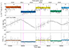 |
Fig. 1. Energy flux and timing parameters of PSR J2021+4026 in the time range from August 5, 2008, to October 6, 2021. In the top panel, error bars are the result of maximum likelihood fits to 30-day intervals. We show the best-fit values (horizontal dashed lines) and the 3σ confidence bands of the flux reported in Table 1, obtained with the phase-averaged spectral analysis (Sect. 3.3) in the time intervals A (red), B (blue), C (yellow), D (green), and E (cyan). Vertical dashed lines indicate the boundaries of these time intervals. In the mid and bottom panels, error bars are obtained with weighted H-tests on 60-day intervals. To enhance the changes in the slope, we report f − k⋅ MJD rather than f, where k = 6.847 × 10⁻⁸ Hz day−1 is an average spin-down rate obtained from a χ2 fit. The solid line and the colored intervals represent the evolution of the spin-down rate predicted using the parameters of Table 2, obtained with the method described in Sect. 3.4. We omitted all points with significance < 5σ. The vertical solid magenta lines at MJD 56028 (April 11, 2012) and MJD 57376 (December 20, 2015) indicate the epochs of the XMM-Newton observations analyzed by Razzano et al. (2023). |
We also monitored the pulsar timing parameters by running a weighted H20-test (Kerr 2011) on 60-day time windows. At this stage, we modeled the phase as the fractional part of a second-order Taylor series,
![Mathematical equation: $$ \begin{aligned} \varphi (t) = \mathrm{frac} \Big [ f(t_0) (t - t_0) + \frac{1}{2} \dot{f} (t_0) (t - t_0)^2 \Big ] \ , \end{aligned} $$](/articles/aa/full_html/2024/05/aa48924-23/aa48924-23-eq5.gif) (4)
(4)
where t0 is the center of each time window and φ ∈ [0, 1]. Photon probabilities were calculated following the simple weights recipe provided by Bruel (2019). We searched for the optimal weight parameter (μw, Eq. (11) of Bruel 2019) with steps of 0.1, and we found that μw = 3.1 maximizes H20. We also varied selection radii between 0 8 and 10° in steps of 0
 1 and found that the test significance is maximized by selecting photons within 4
 4 of the source. The tests produced the optimal values of frequency, f, and spin-down rate, ḟ, as a function of time (middle and bottom panels of Fig. 1). Uncertainties were estimated by bootstrapping samples of the same size for each time interval, repeating the scan and taking the standard deviation of the optimal parameters. We observe that error bars are generally larger when the flux is higher: assuming that 100% of the γ-ray flux is pulsed, this suggests a change in the significance of the pulsation across the mode changes. Although there are clear changes in the slope of f, a direct fit to the points of the time series does not provide a good precision on the ḟ changes, due to the large uncertainties in the high-flux intervals. Instead, a global timing solution (Sect. 3.4) provides a better resolution on ḟ.
3.3. Phase-averaged spectral analysis
To study the changes in the spectral properties, we divided our full data set into five distinct time intervals, labeled A–E. These intervals were defined according to the previously observed events (Allafort et al. 2013; Ng et al. 2016; Takata et al. 2020) as well as the most recent event reported here. The boundaries of the intervals are given in Table 1. We performed the same binned likelihood analysis presented in Sect. 3.2 on the five intervals. We kept all the spectral parameters of PSR J2021+4026 free. The results are provided in Table 1. The best-fit values of the energy flux and its 3σ confidence bands are shown in the top panel of Fig. 1 for comparison with the monitoring results.
Phase-averaged spectral parameters and properties of the pulse profile in different time intervals.
We used the results of the fit to infer the relative flux changes at the four events. We define (e.g., for the first mode change) ΔFγ/Fγ(A − B) = [Fγ(B)−Fγ(A)]/Fγ(A), that is, the ratio between the change in Fγ and the value of Fγ in the previous state. The four relative flux changes are the following: ΔFγ/Fγ(A − B) = − 18.1 ± 1.5%, ΔFγ/Fγ(B − C) = 20 ± 2%, ΔFγ/Fγ(C − D) = − 13.6 ± 1.6% and ΔFγ/Fγ(D − E) = 16 ± 2%. At each transition from low to high γ-ray flux, Fγ always returns to the previous high-flux value within 2σ, that is, Fγ(A)∼Fγ(C)∼Fγ(E). The two low-flux values are also comparable, that is, Fγ(B)∼Fγ(D). In all intervals, the test statistic indicates that our model has a significance > 5σ with respect to a model with constant flux. Indications of spectral softening occur when the flux drops. We observe that the relative increase of Γ is 5.3 ± 1.1% at A–B and 2.9 ± 1.3% at C–D, respectively. Comparable but opposite variations can be observed for the 2014 and 2020 events, in particular −3 ± 1% at B–C and −5.4 ± 1.2% ad D–E. The other parameters, d and b, do not appear to change significantly. For this reason, we also tested a model with b fixed to the value obtained from the global fit, finding that a variable b is preferred with respect to a model with constant b in all the intervals at the > 3σ level. For each time interval, we sampled the multivariate Gaussian distribution defined by the best-fit parameters and the covariance matrix produced by the fit. We computed samples for Ep, dp, and E10, and we estimated their average values and standard deviations. The results reveal that when the flux is low the SED is peaked at lower energies. The relative change in Ep is about –10% at both the A–B and C–D mode changes, while E10 varies by –16% at A–B and by –10% at C–D. On the other hand, the spectral curvature dp does not follow the same trend and is consistent with a constant value. Figure 2 shows the pre-change and post-change best-fit SED at the four events.
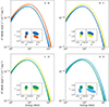 |
Fig. 2. Fitted SEDs of PSR J2021+4026 in intervals A (red), B (blue), C (yellow), D (green), and E (cyan) at the four mode changes. The bands represent the 3σ confidence intervals from a multivariate Gaussian distribution. The inset panels show the 3σ confidence ellipses around the optimal values of the spectral parameters. |
3.4. Timing analysis and pulse profile
We produced a timing model using an unbinned maximum likelihood approach (Ajello et al. 2022). We simultaneously fit the timing model with a model for a stationary noise process whose power spectral density is assumed to follow a power law. The timing model includes terms in the Taylor series up to the second derivative of the frequency,  , although the best-fit value of
  is consistent with zero. To fit the mode changes, we added four glitches, modeled as permanent changes in the frequency derivative, Δ ḟ. Due to the significant level of the timing noise in this pulsar (Razzano et al. 2023), we were not able to fit the epochs of the glitches. Therefore, we manually set them to the MJD of the flux mode changes and kept them fixed. Changes in the absolute phase and in the frequency at the glitches are consistent with zero, therefore we did not include them in the model. The noise model is represented by a truncated Fourier series with 50 terms. The best-fit approach is the same as used in Razzano et al. (2023), but here we extended the validity range of the timing solution to January 2022. The best-fit parameters are reported in Table 2. The bottom panel of Fig. 1 shows the best-fit values of ḟ and its 3σ confidence bands, consistently with how we represented the γ-ray flux in the top panel. For each glitch we also inferred Δḟ/ḟ. For consistency with our definition of ΔFγ/Fγ, we defined this quantity as the ratio between the glitch Δ ḟ and the value of ḟ in the previous state. We estimated the uncertainties by sampling points from the timing parameter space, computing the ratio for each point, then taking the standard deviation of this distribution.
Best-fit parameters of the timing model.
In order to characterize the pulse profile, we calculated photon weights based on the full-mission spectral model of PSR J2021+4026 (Sect. 3.2). We performed an unbinned likelihood fit using the template fitting module included in the PINT Python package (Luo et al. 2021). We modeled the profile with the sum of m phase-wrapped Gaussian components and a constant unpulsed term,
![Mathematical equation: $$ \begin{aligned} \frac{\mathrm{d}N}{\mathrm{d}\varphi } \propto a_0 + \sum _{i=1}^{m} \frac{a_i}{\sqrt{2 \pi \sigma _i^2}} \exp \bigg [ {\frac{1}{2} \frac{(\varphi - \mu _i)^2}{\sigma _i^2}} \bigg ] \ , \end{aligned} $$](/articles/aa/full_html/2024/05/aa48924-23/aa48924-23-eq11.gif) (5)
(5)
where we imposed the normalization condition
 (6)
(6)
We tested different choices of m and found that m = 3 is the simplest model that well describes the pulse profile. A model with m = 4 has a test significance < 3σ when compared with m = 3. We performed two preliminary fits by freeing first only the pulsed-to-constant component ratio, then only the peak locations. This produced a set of starting values for the fit. We then fixed the central peak location and ran the main fit algorithm with all other parameters free. We underline that a unique fit with 10 free parameters could not be performed due to strong parameter correlations. This procedure was applied to each of the five time intervals. We also tested a model with four Gaussian peaks and found that the significance of the extra peak was below 3 sigma. Therefore, we concluded that the three-Gaussian model properly describes the pulse shape.
The phase-folded pulse profile (Fig. 3) reveals two peaks (P1, P2), the second of which is the highest. The two main peaks are separated by ∼0.5 in phase, and they are linked by a wide emission that is similar in shape to the third Vela peak (Abdo et al. 2010). For consistency with previous works (Allafort et al. 2013; Ng et al. 2016) we refer to this third peak as bridge emission (BR). The peaks sit upon a bright constant component. The fraction of flux produced by the peaks is ∼0.3, which means it is smaller than the contribution from the unpulsed component. The off-pulse (OP) region of the light curve, located between P2 and P1, is very narrow and covers < 15% of the rotational period. The unusually broad peaks have been previously explained by the emission geometry required to fit the γ-ray pulsations. For example, Pierbattista et al. (2015) tested different emission models and concluded that the observed light curve is likely the result of either a small magnetic inclination angle with a large viewing angle, or vice versa. This is also consistent with the pulsar being radio-quiet.
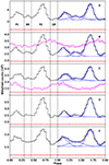 |
Fig. 3. Pulse profile of PSR J2021+4026 in different time intervals. Black solid lines represent the weighted histograms of γ-ray counts produced with phase bins of size 0.04. Only statistical uncertainties are reported. Blue solid lines show the γ-ray best-fit functions. Blue dashed lines represent single Gaussian components. The γ-ray background is estimated from the photon probabilities and is reported with red dashed lines. Vertical dashed lines represent the boundaries of the phase intervals defined in Sect. 3.5. For the sake of completeness, we include the X-ray histograms (magenta solid lines) and best-fit functions (magenta dotted lines) as reported by Razzano et al. (2023). The scales and offsets of the X-ray curves are arbitrary. |
The results of our likelihood fit (Table 1) show that the mode changes affect the overall shape of the pulses. For instance, all amplitude ratios with respect to P2 are lower whenever the γ-ray flux is low, that is, in intervals B and D. The most evident example of this effect is the change in the const-to-P2 ratio, that varies by up to 70% in 2014. Because the amplitude of the constant relative to the main peak decreases when the pulsar switches to a low-flux state, the pulsation significance is higher in intervals B and D, as hinted by the timing monitoring (Sect. 3.2). The separation between P1 and P2 undergoes small variations but no evident correlation with the flux. However, the largest change in the P1–P2 phase lag is ∼8% and occurs again in 2014. There are also indications of variability in the widths of the peaks. In particular, when the flux is low P2 has a larger width, while the bridge emission appears to be narrower. It is difficult to draw conclusions about variability of the bridge component, as its parameters have large uncertainties and are affected by correlations with other parameters.
3.5. Phase-resolved spectral analysis
We searched for more detailed changes by performing a phase-resolved spectral analysis. We subdivided each time interval in four phase (φ) regions: 0–0.3 (P1); 0.3–0.45 (BR); 0.45–0.85 (P2); 0.85–1 (OP). These regions were arbitrarily defined in order to collect at least 95% of the flux from peaks P1 and P2 in all time intervals. Limited phase ranges were reserved to the bridge emission and the off-peak component, as choosing wider boundaries would have increased the contributions from the main peaks. We repeated the spectral analysis outlined in Sect. 3.3 on each phase region independently. At this stage, due to the reduced exposure, we were not able to fit the b parameter. Therefore, we kept it fixed to the value from the full-mission phase-averaged fit, b = 0.35. The results are reported in Table 3.
Phase-resolved spectral parameters in different time intervals and in different phase regions.
Figure 4 presents the flux and spectral index as obtained from the phase-resolved fit in all time intervals. The largest contribution to the overall flux decrease comes from the P1 region (∼46% in 2011, ∼63% in 2018). On the other hand, the flux of P2 is stable and does not contribute significantly to the overall change. The flux evolution follows the same trend observed in the phase-averaged analysis in all phase regions except P2. The spectral index is not significantly phase-dependent, with the exceptions of intervals B and C where the OP spectrum appears softer. Because the uncertainties are large, this apparent change may be a statistical fluctuation. We also report the inferred values of Ep, dp and E10 in Fig. 4. We observe that the trend of the Ep and E10 variations is consistent with the phase-averaged analysis. The P1 and BR spectra show the largest relative Ep jumps, while in OP the value of the parameter is systematically lower. We observe consistent variations of E10 in P1, BR, and P2, while the spectrum of OP has a lower E10 at all phases. Finally, dp appears to be phase-independent and remains time-independent at all phases.
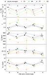 |
Fig. 4. Measured physical parameters obtained from the phase-averaged and phase-resolved spectral analysis in different time intervals. Values and uncertainties are reported in Tables 1 and 3. Error bars are grouped according to the time intervals and connected by dotted lines of consistent color. The horizontal axis is not to scale. |
4. Discussion
We have presented an analysis of PSR J2021+4026, the only known variable γ-ray pulsar, using Fermi-LAT data spanning more than 13 years. In this time period, we observed two full cycles. Each cycle consists of a first mode change, where the γ-ray flux decreased and the frequency derivative increased, followed by a second mode change after ∼3 years nearly returning to the previous state. The mode changes do not conform to the typical glitch behavior seen in many rotation-powered pulsars, which usually involves a positive change in frequency. Instead, PSR J2021+4026 shows no sudden spin up at the mode changes. Moreover, the typical jump in ḟ is smaller compared to the values measured for PSR J2021+4026, and no γ-ray flux change is observed in correlation with the usual glitches. Takata et al. (2020) discuss several models for the PSR J2021+4026 mode changes, including a change in the magnetic inclination angle, a change in the magnetospheric current, a change in surface magnetic field structure, precession of the NS, and a magnetar twisted-field model, as well as a standard pulsar glitch model. They favor a change in surface magnetic field structure, which could be due to stresses on the crust that cause cracking and movement of the surface field lines. Figure 6 of Takata et al. (2020) shows that the Δ ḟ and ḟ observed for PSR J2021+4026 lie on the Δ ḟ vs. ḟ correlation seen for both pulsar glitches and pulsars showing correlated ḟ and radio pulse profile changes (Lyne et al. 2010), suggesting that the PSR J2021+4026 mode changes could be related to the Lyne et al. (2010) mode changes and could also involve crustal shifts.
The X-ray pulsations of PSR J2021+4026 exhibit one broad peak (panels B and C of Fig. 3). With a multiwavelength timing analysis, Razzano et al. (2023) revealed that the position of the X-ray peak relative to highest γ-ray peak (P2) shifted by 0.21 ± 0.02 across the 2014 mode change. They also reported that the X-ray spectrum in the 0.3–12 keV energy range is well described by a two-component model defined as a blackbody plus a power law. In particular, the blackbody component has a flux of (11.0 ± 2.4)×10−14 erg cm−2 s−1, while the power-law component has a flux of (3.2 ± 0.7)×10−14 erg cm−2 s−1. This implies that the thermal emission dominates the X-ray flux, and ∼80% of the X rays must be emitted at the NS surface. Razzano et al. (2023) outlined a possible model for the change in ḟ and γ-ray flux at the B–C mode change, as a change in the magnetospheric conductivity (or equivalently, the pair multiplicity). To explain the results of their analysis, as well as a possible change in pair multiplicity, they speculated that a changing quadrupole field component near the NS surface could cause the current sheet of the dipole field, which is dominant far from the NS, to connect to a different pole of the quadrupole. Different conditions for pair production at the different poles of the quadrupole could provide higher or lower conductivity and consequently change ḟ and the γ-ray flux. Here, we develop this idea more quantitatively.
To physically connect the changes in ḟ to the conductivity, we invoke results of global pulsar magnetosphere models. Dissipative global models assume a macroscopic conductivity σ that relates the current density J to the electric field parallel to the magnetic field, E∥ (Kalapotharakos et al. 2012),
 (7)
(7)
where ρ is the charge density and E and B are the total electric and magnetic fields. The first term in Eq. (7) is the drift velocity contribution to the current. Li et al. (2012) give an expression (in their Eq. (9)) for the pulsar spin-down luminosity L in terms of the σ of their dissipative global models,
 (8)
(8)
for relatively high σ near to the force-free (FF) case, where L0 is 3/2 times the spin-down power of a vacuum rotator, Ω is the pulsar rotation rate, and α is the magnetic inclination angle. We assume that Ω is constant since there is no observed change in f at the mode changes. Because the variations in the shape and position of the peaks are small, we also assume that α does not change. Writing L = −4π2I f ḟ, we can deduce that Δḟ/ḟ = 0.6 Ω (L0/L) Δσ/σ. In the near-FF condition we approximate L/L0 ∼ 1 + sin2α (Li et al. 2012), and setting α = 45°, which would reproduce the γ-ray profile (Kalapotharakos et al. 2014), we get Δḟ/ḟ = 2.5f Δσ/σ. Using the observed frequency f and the fractional changes  listed in Table 2 we get the values of Δσ/σ reported in Table 4.
Measured and inferred parameters for the dissipative magnetosphere model.
The macroscopic σ in the dissipative models physically reflects the density of pair plasma in the magnetosphere that is able to screen the E∥ and reach closer to an FF state where σ → ∞. An increase in σ in the A–B and C–D mode transitions then implies a magnetosphere slightly closer to FF. In a near-FF magnetosphere, a state that it is believed all Fermi-LAT pulsars must approach (Kalapotharakos et al. 2014), the current will adjust to the FF current JFF with any small change in σ. It has been shown that the global current controls the polar cap pair creation rather than the pair creation controlling the global current (Timokhin 2010). Therefore, Eq. (7) implies that ΔE∥/E∥ = −Δσ/σ if J = JFF is constant. Consequently, increases in conductivity will screen more of the E∥, assuming that ρ and the field strengths do not change. The observed changes in the P1-to-P2 peak amplitude ratio suggest a change also in the spatial distribution of E∥ affecting the emissivity asymmetrically, or variations in the local magnetic field structure.
A decrease in E∥ will decrease the particle acceleration and thus, potentially the γ-ray luminosity. Both global dissipative models and more recent kinetic plasma (particle-in-cell, PIC) simulations of global pulsar magnetospheres (Kalapotharakos et al. 2018; Philippov & Spitkovsky 2018) show that in the near-FF state, most particle acceleration takes place near the current sheet beyond the light cylinder. The current sheet is therefore the site of the γ-ray emission, and the variations in the width of the peaks observed across the PSR J2021+4026 mode changes may be due to changes in the size of the acceleration regions. However, the γ-ray emission mechanism is currently under debate, with some favoring curvature radiation (Kalapotharakos et al. 2018) and others favoring synchrotron radiation (Philippov & Spitkovsky 2018) for the GeV emission. This disagreement results from the different interpretations of the PIC models, which cannot simulate realistically high values of pulsar surface magnetic field strengths. It has been shown that all Fermi-LAT pulsars lie on the same fundamental plane if they are emitting CR near the light cylinder (Kalapotharakos et al. 2019, 2022). Therefore, for the estimates of this paper, we assume curvature radiation (CR) for the GeV emission of PSR J2021+4026. Moreover, we assume that the CR emitting particles have reached the radiation-reaction limit, where the energy gain from E∥ acceleration balances the energy loss to CR. In CR reaction limit, which we assume holds in this case, the CR cutoff energy in the spectrum  (Kalapotharakos et al. 2019). Therefore, from the dependency derived above, ΔE∥/E∥ = −Δσ/σ, we have ΔECR/ECR = (3/4) ΔE∥/E∥.
The cutoff energy can be made explicit in the spectral photon distribution with a different choice of parameters (Eq. (14) in 3PC). If we assume that the cutoff energy of the parametric function dN/dE is approximately the CR cutoff energy, then from Eqs. (17) and (21) of 3PC we get a relation between Ep, ECR and the spectral parameters. Since there are no indications of changes in b and d, we assume that Ep is only a function of ECR and Γ. With a linear approximation we get
![Mathematical equation: $$ \begin{aligned} \frac{\Delta E_{\rm p}}{E_{\rm p}} = \frac{\Delta E_{\rm CR}}{E_{\rm CR}} - \frac{1}{b} \ \Bigg [ \frac{\Gamma }{2 - \Gamma + d / b} \Bigg ] \frac{\Delta \Gamma }{\Gamma } \ \end{aligned} $$](/articles/aa/full_html/2024/05/aa48924-23/aa48924-23-eq17.gif) (9)
(9)
and we can infer the predicted changes ΔEp/Ep from the ΔECR/ECR computed above and from the measured ΔΓ/Γ. We can compare our predictions (Table 4) with the observed changes in phase-averaged Ep from the values listed in Table 1 and shown in Fig. 4. The predicted changes are in the same direction as the observed variations. The predicted value for the (B − C) change agrees with that observed within the errors, while the prediction for the (A − B) change is off by ∼2σ.
Next, we define Fγ = ∫E(dN/dE)dE, and we note that it can be related to Ep through Eqs. (1) and (2). We can therefore derive the change in Fγ as a function of ΔEp/Ep,
 (10)
(10)
where
![Mathematical equation: $$ \begin{aligned} \Lambda = \frac{d}{b} \log \Bigg [ \Bigg ( \frac{E_{\rm p}}{E_0} \Bigg )^b - \frac{b^2}{d} \Bigg ] \, + \, \frac{b}{2}\, \Bigg [ \Bigg ( \frac{E_{\rm p}}{E_0} \Bigg )^b - \frac{b^2}{d} \Bigg ]^{-1} \ . \end{aligned} $$](/articles/aa/full_html/2024/05/aa48924-23/aa48924-23-eq19.gif) (11)
(11)
In Eq. (10), if we take ΔEp/Ep from our predicted ECR changes given above, and d, b, and Ep from the global values reported in Sect. 3.2, we can estimate the fractional γ-ray flux changes ΔFγ/Fγ. The predictions show that the effect of a negative ΔEp/Ep produces variations that are smaller in amplitude and of opposite sign compared to the observed ΔFγ/Fγ. We also added a term ∝Δd/d to Eq. (10) and we proved that the results do not change significantly. This implies that we cannot quantitatively reproduce the measured flux changes if we only assume fluctuations in the conductivity. Therefore, we must allow for variations in other quantities.
We can state that in a near-FF magnetosphere, where J stays constant to the FF value, the measured change in Fγ is likely the result of variations in the effective magnetic field (Eq. (7)). We recall the theoretical fundamental plane relation in the CR-regime,  , where Lγ is the γ-ray luminosity, ECR is the spectral cutoff energy, B* is the surface magnetic field, and L = −4π2I f ḟ (Kalapotharakos et al. 2019). As pointed out by Kalapotharakos et al. (2022), the high-energy part of the γ-ray spectrum is well probed by the E10 characteristic energy, so that ΔE10/E10 ∼ ΔECR/ECR. Moreover, assuming dipole radiation in vacuum, we can approximate ΔB∗/B∗ ∼ 0.5 Δḟ/ḟ, corresponding to a small change in B* by ∼2.9% in A–B, ∼1.2% in C–D. We can thus write
 (12)
(12)
and using the measured quantities reported in Table 1 we obtain the ΔLγ/Lγ of Table 4. The inferred changes are remarkably close to the measured ΔFγ/Fγ, and this implies that a field reconfiguration must occur in order for the pulsar to remain on the fundamental plane across the mode changes.
To interpret the apparent field reconfiguration at the PSR J2021+4026 mode changes, we would need to explore the geometry of the magnetic field. In particular, we need to account for the small increase in the surface field B* implied from the pulsar fundamental plane, and for the phase change of the X-ray pulse observed by Razzano et al. (2023). For the purpose of this discussion, we limit ourselves to study an analytical model for the magnetic field in vacuum (Kalapotharakos et al. 2021). The model assumes that the global magnetic field at large distances from the NS is a dipole but near the star a quadrupole field component dominates. The dipole component of the field determines the position and geometry of the current sheet, where the γ-ray emission is produced. This is consistent with the observed constancy of the γ-ray peak phases and only subtle changes in the profile. We set up a coordinate system with the origin in the NS center and the z axis aligned to the rotation axis. We assume that the dipole (D) and quadrupole (Q) moments are both centered at the origin, and their orientations are each defined by a colatitude α and an azimuthal angle ϕ. Without loss of generality, we always set the azimuthal angle of the dipole ϕD = 0, and we leave the other angles free to vary. The ratio between the quadrupole and dipole surface fields is also free, and thus the full set of free parameters is (αD, αQ, ϕQ, BQ/BD). We simulate the quadrupole plus dipole configuration as follows. We start by creating a grid of 216 equally spaced points on the NS surface. Each point corresponds to a unit surface area of 2−16 ⋅ 4πR*2, where R* is the NS radius. Starting from each point on the surface, we iteratively build a magnetic field line. At each iteration i we compute the total magnetic field Bi at the point xi, then we make a step of size 0.01 R* in the direction of the field, that is, xi + 1 = xi + 0.01 R*Bi/|Bi|. We stop when the path crosses the light cylinder (open field lines) or goes back down and touches the surface (closed field lines). For each line we record the strength and the inclination angle of the field at the surface. At the end of the simulation, we look for polar caps, defined as contiguous regions containing open field lines. For each polar cap we compute the area, the average magnetic field at the surface and the field inclination at the geometrical center. We explore a range of orientations and relative strengths of the quadrupole, keeping the dipole constant. We assume that the dipole has inclination of αD = 45° and our viewing angle is near ζ = 90° (Pierbattista et al. 2015). We also explored the αD = 60° case and the results are very similar. The choice of a constant αD is supported by the fact that the peak positions are substantially stable, indicating that the dipole is fundamentally unaffected by the magnetospheric mode. In general, the quadrupole has four poles, but in some configurations not all of them connect to the open field lines of the dipole. We assume that only polar caps that are open can generate current that heats the surface to produce thermal X-rays. Searching for cases where the poles of the quadrupole that connect to the open dipole lines at larger altitude change by 0.21 in phase, as observed for the X-ray pulse, we focused on configurations where the quadrupole changes rotational phase within a specific range but not inclination angle.
Figure 5 shows two orientations of the quadrupole of relative strength BQ/BD = 5, ϕQ = 95° and ϕQ = 180°, that produce open polar caps seen by an observer at ζ ∼ 90° that are approximately 0.21 apart in phase. In the Mollweide projection plots, the poles of the dipole are at 0° and 180° at ζ = 45° latitude. The first γ-ray peak, P1, would be at approximately 0.15 in phase or at 42° (see Kalapotharakos et al. 2014). The left-hand panels represent the field configuration and polar cap positions during interval B, where the X-ray pulse is at approximately 0.14 in phase later than the first γ-ray peak (see Fig. 1 of Razzano et al. 2023). The right-hand panels represent the fields and polar caps for interval C, where the X-ray pulse is 0.35 in phase later than P1. In the first case, three of the quadrupole poles connect to the dipole open field lines, and thus eventually to the current sheet, with two of the poles connected to the current sheet from one rotational hemisphere. In the second configuration, only two poles of the quadrupole connect to the open dipole field. The first case then would have three heated polar caps, only two of which are likely visible to one observer with ζ ∼ 90°, and three polar caps supplying electron-positron pairs to the current sheet. The surface magnetic field strength is slightly lower over the poles in the first configuration (interval B) than in the second configuration (interval C), while the curvature of the field lines over the poles in interval B is smaller, since the two poles are connecting to the same pole of the dipole. This could allow pairs to be created with smaller mean-free paths since the one-photon pair threshold depends on the angle of the photon to the magnetic field, as well as the field strength. This configuration would therefore represent interval B, having a higher conductivity, a higher ḟ, and a lower γ-ray flux. The P1 peak in the γ-ray profile comes from the part of the current sheet that is connected to two quadrupole poles in interval B and one quadrupole pole in interval C. It would therefore be expected to show the largest change in flux and spectrum. In fact we see in Fig. 4 that P1 has the largest changes in flux and Ep while P2 has much smaller, or no, changes in flux of Ep. In both configurations, the estimated area of the polar cap near the equator is ∼109 cm2, corresponding to a radius of ∼300 m. This is consistent with the size of the thermal emitting region observed by Razzano et al. (2023).
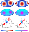 |
Fig. 5. Magnetic field configurations for a dipole with (αD, φD) = (45° ,0° ) and a quadrupole with two different orientations. Left: (αQ, φQ) = (80° ,95° ). Right: (αQ, φQ) = (80° ,180° ). BQ/BD = 5 in both cases. The top and middle panels show the angle of the surface magnetic field with respect to the radial direction, cos θB, and the relative magnetic field strength at the surface, B/BD, in Mollweide projection. The maps cover the whole NS surface with latitudes in the range [−90°, 90°] and longitudes in the range [−180°, 180°]. The boundaries of the polar caps are shown with solid black lines. In the 3D representations, we represented closed field lines in blue, open field lines in red. The green arrow indicates the rotation axis of the NS. All distances are scaled by the stellar radius, R*. |
The cause of the mode changes is uncertain. Takata et al. (2020) suggest that strains on the stellar crust due to moving vortex lines in the superconducting core exceed the crustal elastic stresses, causing the crust to crack (Ruderman 1991). The crust will then move to relieve the stress, and they estimate that for an interval between successive displacements of τ ∼ 7 years for PSR J2021+4026 a crustal displacement of about 1 m would result. Our simple toy model outlined above assumes a quadrupole changing phase by 85°. This implies that a larger movement would be necessary to reconfigure the surface fields so that the quadrupole poles disconnect or reconnect with the poles of the dipole. However, our model is only illustrative and the real surface field could be more complex, containing higher multipoles allowing small displacements of the crust to cause large reconfiguration of the global field. A long-term evolution of the magnetic field is also expected in highly magnetized NSs due to Lorentz forces acting on the electron superfluid component (Hall drift, Goldreich & Reisenegger 1992). This effect favors the formation and evolution of small-scale structures in the internal current distribution, ultimately determining the geometry of the magnetic field. However, due to the complexity of Hall dynamics, we cannot yet say whether this effect could produce abrupt events such as the PSR J2021+4026 mode changes.
Since PSR J2021+4026 is a radio-quiet pulsar, we should not see the radio pulse in either mode. However, we must see one heated polar cap in each mode and it is believed that the radio emission is produced above the polar caps. A possible reason for the non-detection of the radio pulses is that, if they are produced at altitudes of 50–100 stellar radii, the distortions of the field lines by the quadrupole cause the emission to be beamed in a direction away from the dipole and quadrupole axes. The X-ray emission is thermal, therefore more isotropic and is visible over a wider range of angles.
5. Conclusions
We have reported on the results of an updated Fermi-LAT analysis of the variable γ-ray pulsar PSR J2021+4026. We performed a full phase-averaged and phase-resolved γ-ray spectral analysis, studying the properties of the γ-ray emission in detail. We investigated a significant mode change, which occurred around June 2020. This event produced an increase in the γ-ray flux by 16 ± 2% and a drop in the spin-down rate by 3.0 ± 0.6%. We also reported indications of changes in the phase-averaged spectrum and an increase in the pulsation significance concurrent with the flux drops. The phase-resolved analysis suggests that the mode change affects the peaks of the light curve differently, implying an asymmetric variation in the structure of the magnetosphere.
In an attempt to interpret the nature of PSR J2021+4026, we used the measured relative change in ḟ to predict the observed flux drop. Under the hypothesis of pure CR emission in a dissipative magnetosphere, we computed the approximated flux variations produced by a change in the global conductivity. The predictions are in disagreement with the observations, indicating that changes in the surface magnetic field also contribute to the flux modes. This hypothesis is consistent with the observed X-ray phase shift (Razzano et al. 2023) observed across the 2014 mode change. For this reason, we invoked and explored a model for a multipolar magnetic field in vacuum, finding a configuration that qualitatively agrees with both the phase-averaged and the phase-resolved spectral analysis. However, this model does not account for the microphysics linking the fields to other electrodynamical quantities, and the derivation of a self-consistent radiative model to predict the PSR J2021+4026 spectral changes will be the topic of future work. Moreover, because the observed changes in the timing parameters differ from the classic glitch phenomenology, the mechanism driving the PSR J2021+4026 mode changes remains unknown. Therefore, although our interpretation is still qualitative, it should nevertheless pave the way to further research.
In order to understand the physics of the mode changes more fully, it is essential to make observations of the X-ray pulse within each mode as well as between modes. NASA’s Neutron Star Interior Composition Explorer (NICER; Gendreau et al. 2016) may be the ideal instrument to achieve an accurate absolute X-ray timing, enabling joint X-ray and γ-ray light curve fitting. Therefore, a continuous monitoring of PSR J2021+4026 by Fermi-LAT is the key to get further insight into the physics of variable γ-ray pulsars.
Public list of LAT-detected γ-ray pulsars: https://confluence.slac.stanford.edu/display/GLAMCOG/Public+List+of+LAT-Detected+Gamma-Ray+Pulsars
There is a significant discrepancy between the characteristic spin-down age of PSR J2021+4026 and the estimated age of SNR G 78.2+2.1 of < 10 kyr (Leahy et al. 2013).
Acknowledgments
The Fermi-LAT Collaboration acknowledges generous ongoing support from a number of agencies and institutes that have supported both the development and the operation of the LAT as well as scientific data analysis. These include the National Aeronautics and Space Administration and the Department of Energy in the United States, the Commissariat à l’Energie Atomique and the Centre National de la Recherche Scientifique/Institut National de Physique Nucléaire et de Physique des Particules in France, the Agenzia Spaziale Italiana and the Istituto Nazionale di Fisica Nucleare in Italy, the Ministry of Education, Culture, Sports, Science and Technology (MEXT), High Energy Accelerator Research Organization (KEK) and Japan Aerospace Exploration Agency (JAXA) in Japan, and the K. A. Wallenberg Foundation, the Swedish Research Council and the Swedish National Space Board in Sweden. Additional support for science analysis during the operations phase is gratefully acknowledged from the Istituto Nazionale di Astrofisica in Italy and the Centre National d’Études Spatiales in France. This work performed in part under DOE Contract DE-AC02-76SF00515. Work at NRL is supported by NASA.
References
- Abdo, A. A., Ackermann, M., Ajello, M., et al. 2009, Science, 325, 840 [Google Scholar]
- Abdo, A. A., Ackermann, M., Ajello, M., et al. 2010, ApJ, 713, 154 [NASA ADS] [CrossRef] [Google Scholar]
- Abdollahi, S., Acero, F., Baldini, L., et al. 2022, ApJS, 260, 53 [NASA ADS] [CrossRef] [Google Scholar]
- Ajello, M., Atwood, W. B., Baldini, L., et al. 2022, Science, 376, 521 [NASA ADS] [CrossRef] [Google Scholar]
- Allafort, A., Baldini, L., Ballet, J., et al. 2013, ApJ, 777, L2 [NASA ADS] [CrossRef] [Google Scholar]
- Atwood, W. B., Albert, A., Baldini, L., et al. 2009, ApJ, 697, 1071 [NASA ADS] [CrossRef] [Google Scholar]
- Atwood, W., Albert, A., Baldini, L., et al. 2013, arXiv e-prints [arXiv:1303.3514] [Google Scholar]
- Bruel, P. 2019, A&A, 622, A108 [NASA ADS] [CrossRef] [EDP Sciences] [Google Scholar]
- Bruel, P., Burnett, T. H., Digel, S. W., et al. 2018, arXiv e-prints [arXiv:1810.11394] [Google Scholar]
- Fiori, A., Razzano, M., Saz Parkinson, P., & Mignani, R. 2023, PoS, ECRS, 110 [Google Scholar]
- Gendreau, K. C., Arzoumanian, Z., Adkins, P. W., et al. 2016, SPIE Conf. Ser., 9905, 99051H [NASA ADS] [Google Scholar]
- Goldreich, P., & Reisenegger, A. 1992, ApJ, 395, 250 [NASA ADS] [CrossRef] [Google Scholar]
- Hartman, R. C., Bertsch, D. L., Bloom, S. D., et al. 1999, ApJS, 123, 79 [CrossRef] [Google Scholar]
- Kalapotharakos, C., Kazanas, D., Harding, A., & Contopoulos, I. 2012, ApJ, 749, 2 [NASA ADS] [CrossRef] [Google Scholar]
- Kalapotharakos, C., Harding, A. K., & Kazanas, D. 2014, ApJ, 793, 97 [Google Scholar]
- Kalapotharakos, C., Brambilla, G., Timokhin, A., Harding, A. K., & Kazanas, D. 2018, ApJ, 857, 44 [NASA ADS] [CrossRef] [Google Scholar]
- Kalapotharakos, C., Harding, A. K., Kazanas, D., & Wadiasingh, Z. 2019, ApJ, 883, L4 [NASA ADS] [CrossRef] [Google Scholar]
- Kalapotharakos, C., Wadiasingh, Z., Harding, A. K., & Kazanas, D. 2021, ApJ, 907, 63 [NASA ADS] [CrossRef] [Google Scholar]
- Kalapotharakos, C., Wadiasingh, Z., Harding, A. K., & Kazanas, D. 2022, ApJ, 934, 65 [NASA ADS] [CrossRef] [Google Scholar]
- Kerr, M. 2011, ApJ, 732, 38 [NASA ADS] [CrossRef] [Google Scholar]
- Landecker, T. L., Roger, R. S., & Higgs, L. A. 1980, A&AS, 39, 133 [Google Scholar]
- Leahy, D. A., Green, K., & Ranasinghe, S. 2013, MNRAS, 436, 968 [NASA ADS] [CrossRef] [Google Scholar]
- Li, J., Spitkovsky, A., & Tchekhovskoy, A. 2012, ApJ, 746, 60 [Google Scholar]
- Lin, L. C. C., Hui, C. Y., Hu, C. P., et al. 2013, ApJ, 770, L9 [Google Scholar]
- Luo, J., Ransom, S., Demorest, P., et al. 2021, ApJ, 911, 45 [NASA ADS] [CrossRef] [Google Scholar]
- Lyne, A., Hobbs, G., Kramer, M., Stairs, I., & Stappers, B. 2010, Science, 329, 408 [NASA ADS] [CrossRef] [Google Scholar]
- Ng, C. W., Takata, J., & Cheng, K. S. 2016, ApJ, 825, 18 [CrossRef] [Google Scholar]
- Philippov, A. A., & Spitkovsky, A. 2018, ApJ, 855, 94 [NASA ADS] [CrossRef] [Google Scholar]
- Pierbattista, M., Harding, A. K., Grenier, I. A., et al. 2015, A&A, 575, A3 [NASA ADS] [CrossRef] [EDP Sciences] [Google Scholar]
- Prokhorov, D. A., & Moraghan, A. 2023, MNRAS, 519, 2680 [Google Scholar]
- Ray, P. S., Kerr, M., Parent, D., et al. 2011, ApJS, 194, 17 [NASA ADS] [CrossRef] [Google Scholar]
- Razzano, M., Fiori, A., Saz Parkinson, P. M., et al. 2023, A&A, 676, A91 [NASA ADS] [CrossRef] [EDP Sciences] [Google Scholar]
- Ruderman, M. 1991, ApJ, 366, 261 [CrossRef] [Google Scholar]
- Shaw, B., Stappers, B. W., Weltevrede, P., et al. 2023, MNRAS, 523, 568 [CrossRef] [Google Scholar]
- Smith, D. A., Abdollahi, S., Ajello, M., et al. 2023, ApJ, 958, 191 [NASA ADS] [CrossRef] [Google Scholar]
- Standish, E. M. 1998, A&A, 336, 381 [NASA ADS] [Google Scholar]
- Takata, J., Shibata, S., Hirotani, K., et al. 2020, ApJ, 890, 16 [NASA ADS] [CrossRef] [Google Scholar]
- Timokhin, A. N. 2010, MNRAS, 408, 2092 [NASA ADS] [CrossRef] [Google Scholar]
- Weisskopf, M. C., Swartz, D. A., Carramiñana, A., et al. 2006, ApJ, 652, 387 [NASA ADS] [CrossRef] [Google Scholar]
- Weisskopf, M. C., Romani, R. W., Razzano, M., et al. 2011, ApJ, 743, 74 [NASA ADS] [CrossRef] [Google Scholar]
- Zhao, J., Ng, C. W., Lin, L. C. C., et al. 2017, ApJ, 842, 53 [NASA ADS] [CrossRef] [Google Scholar]
All Tables
Phase-averaged spectral parameters and properties of the pulse profile in different time intervals.
Phase-resolved spectral parameters in different time intervals and in different phase regions.
All Figures
|
Fig. 1. Energy flux and timing parameters of PSR J2021+4026 in the time range from August 5, 2008, to October 6, 2021. In the top panel, error bars are the result of maximum likelihood fits to 30-day intervals. We show the best-fit values (horizontal dashed lines) and the 3σ confidence bands of the flux reported in Table 1, obtained with the phase-averaged spectral analysis (Sect. 3.3) in the time intervals A (red), B (blue), C (yellow), D (green), and E (cyan). Vertical dashed lines indicate the boundaries of these time intervals. In the mid and bottom panels, error bars are obtained with weighted H-tests on 60-day intervals. To enhance the changes in the slope, we report f − k⋅ MJD rather than f, where k = 6.847 × 10⁻⁸ Hz day−1 is an average spin-down rate obtained from a χ2 fit. The solid line and the colored intervals represent the evolution of the spin-down rate predicted using the parameters of Table 2, obtained with the method described in Sect. 3.4. We omitted all points with significance < 5σ. The vertical solid magenta lines at MJD 56028 (April 11, 2012) and MJD 57376 (December 20, 2015) indicate the epochs of the XMM-Newton observations analyzed by Razzano et al. (2023). |
| In the text | |
|
Fig. 2. Fitted SEDs of PSR J2021+4026 in intervals A (red), B (blue), C (yellow), D (green), and E (cyan) at the four mode changes. The bands represent the 3σ confidence intervals from a multivariate Gaussian distribution. The inset panels show the 3σ confidence ellipses around the optimal values of the spectral parameters. |
| In the text | |
|
Fig. 3. Pulse profile of PSR J2021+4026 in different time intervals. Black solid lines represent the weighted histograms of γ-ray counts produced with phase bins of size 0.04. Only statistical uncertainties are reported. Blue solid lines show the γ-ray best-fit functions. Blue dashed lines represent single Gaussian components. The γ-ray background is estimated from the photon probabilities and is reported with red dashed lines. Vertical dashed lines represent the boundaries of the phase intervals defined in Sect. 3.5. For the sake of completeness, we include the X-ray histograms (magenta solid lines) and best-fit functions (magenta dotted lines) as reported by Razzano et al. (2023). The scales and offsets of the X-ray curves are arbitrary. |
| In the text | |
|
Fig. 4. Measured physical parameters obtained from the phase-averaged and phase-resolved spectral analysis in different time intervals. Values and uncertainties are reported in Tables 1 and 3. Error bars are grouped according to the time intervals and connected by dotted lines of consistent color. The horizontal axis is not to scale. |
| In the text | |
|
Fig. 5. Magnetic field configurations for a dipole with (αD, φD) = (45° ,0° ) and a quadrupole with two different orientations. Left: (αQ, φQ) = (80° ,95° ). Right: (αQ, φQ) = (80° ,180° ). BQ/BD = 5 in both cases. The top and middle panels show the angle of the surface magnetic field with respect to the radial direction, cos θB, and the relative magnetic field strength at the surface, B/BD, in Mollweide projection. The maps cover the whole NS surface with latitudes in the range [−90°, 90°] and longitudes in the range [−180°, 180°]. The boundaries of the polar caps are shown with solid black lines. In the 3D representations, we represented closed field lines in blue, open field lines in red. The green arrow indicates the rotation axis of the NS. All distances are scaled by the stellar radius, R*. |
| In the text | |
Current usage metrics show cumulative count of Article Views (full-text article views including HTML views, PDF and ePub downloads, according to the available data) and Abstracts Views on Vision4Press platform.
Data correspond to usage on the plateform after 2015. The current usage metrics is available 48-96 hours after online publication and is updated daily on week days.
Initial download of the metrics may take a while.