| Issue |
A&A
Volume 676, August 2023
|
|
|---|---|---|
| Article Number | A91 | |
| Number of page(s) | 10 | |
| Section | Stellar structure and evolution | |
| DOI | https://doi.org/10.1051/0004-6361/202345873 | |
| Published online | 10 August 2023 | |
Multiwavelength observations of PSR J2021+4026 across a mode change reveal a phase shift in its X-ray emission
1
Università di Pisa and Istituto Nazionale di Fisica Nucleare, Sezione di Pisa, 56127 Pisa, Italy
e-mail: massimiliano.razzano@unipi.it
2
Santa Cruz Institute for Particle Physics, Department of Physics and Department of Astronomy and Astrophysics, University of California at Santa Cruz, Santa Cruz, CA, 95064
USA
3
INAF-Istituto di Astrofisica Spaziale e Fisica Cosmica Milano, via E. Bassini 15, 20133 Milano, Italy
4
Kepler Institute of Astronomy, University of Zielona Góra, Lubuska 2, 65-265 Zielona Góra, Poland
5
Istituto Universitario di Studi Superiori (IUSS), 27100 Pavia, Italy
6
Los Alamos National Laboratory, Los Alamos, NM, 87545
USA
7
Space Science Division, Naval Research Laboratory, Washington, DC, 20375-5352
USA
8
INAF Osservatorio Astronomico di Roma, Via Frascati 33, 00078 Monte Porzio Catone, Roma, Italy
Received:
9
January
2023
Accepted:
31
May
2023
Context. We have investigated the multiwavelength emission of PSR J2021+4026, the only isolated γ-ray pulsar known to be variable, which in October 2011 underwent a simultaneous change in γ-ray flux and spin-down rate, followed by a second mode change in February 2018. Multiwavelength monitoring is crucial to understand the physics behind these events and how they may have affected the structure of the magnetosphere.
Aims. The monitoring of pulse profile alignment is a powerful diagnostic tool for constraining magnetospheric reconfiguration. We aim to investigate timing or flux changes related to the variability of PSR J2021+4026 via multiwavelength observations, including γ-ray observations from Fermi-LAT, X-ray observations from XMM-Newton, and a deep optical observation with the Gran Telescopio Canarias.
Methods. We performed a detailed comparison of the timing features of the pulsar in γ and X-rays and searched for any change in phase lag between the phaseogram peaks in these two energy bands. Although previous observations did not detect a counterpart in visible light, we also searched for optical emission that might have increased due to the mode change, making this pulsar detectable in the optical.
Results. We have found a change in the γ-to X-ray pulse profile alignment by 0.21 ± 0.02 in phase, which indicates that the first mode change affected different regions of the pulsar magnetosphere. No optical counterpart was detected down to g′ = 26.1 and r′ = 25.3.
Conclusions. We suggest that the observed phase shift could be related to a reconfiguration of the connection between the quadrupole magnetic field near the stellar surface and the dipole field that dominates at larger distances. This is consistent with the picture of X-ray emission coming from the heated polar cap and with the simultaneous flux and frequency derivative change observed during the mode changes.
Key words: gamma rays: stars / pulsars: individual: J2021+4026 / pulsars: general / stars: magnetic field
© The Authors 2023
 Open Access article, published by EDP Sciences, under the terms of the Creative Commons Attribution License (https://creativecommons.org/licenses/by/4.0), which permits unrestricted use, distribution, and reproduction in any medium, provided the original work is properly cited.
This article is published in open access under the Subscribe to Open model. Subscribe to A&A to support open access publication.
1. Introduction
The Fermi Large Area Telescope (LAT; Atwood et al. 2009) sparked a revolution in pulsar astrophysics, with the detection of ∼300 γ-ray pulsars1. Among the Fermi-LAT radio-quiet pulsars, PSR J2021+4026 is particularly interesting for its intrinsically variable behaviour. It was discovered in blind periodicity searches of the Fermi-LAT gamma-ray source coincident with the unidentified EGRET source 3EG J2020+4017 (Abdo et al. 2009). Deep Chandra observations helped to pinpoint the X-ray counterpart (Weisskopf et al. 2011), whose pulsed emission was later detected by XMM-Newton (Lin et al. 2013). The X-ray phaseogram shows a single broad pulse, while the γ-ray one shows two peaks separated by ∼0.5 in phase.
PSR J2021+4026 is seen within the radio shell of the Gamma Cygni (G 78.2+2.1) supernova remnant (SNR) in one of the richest and most complex regions of the γ-ray sky (Higgs et al. 1977). Its spin frequency (f0 ∼ 3.8 Hz) and frequency derivative (f1 ∼ −8 × 10⁻¹³ Hz s−1) point to an energetic, rotation-powered pulsar (characteristic age τc = 77 kyr, spin-down power ĖSD ∼ 1035 erg s−1). Having never been detected in radio (Ray et al. 2011), there is no estimate of the pulsar distance from the dispersion measure (Cordes & Lazio 2002), while kinematic models imply a distance of 1.5 ± 0.4 kpc for the SNR (Landecker et al. 1980), yielding an indirect distance estimate for the pulsar based on the assumed association with the SNR. The pulsar drew attention when it exhibited a simultaneous change in γ-ray flux and frequency derivative f1 detected by Fermi-LAT in October 2011 (MJD 55850) (Allafort et al. 2013). Changes in pulsar frequency derivative have been observed for instance in PSR B0540-69 (Marshall et al. 2015), which did not show any simultaneous change in γ-ray flux, however. This mode changing is still unique among the population of γ-ray pulsars, and therefore, PSR J2021+4026 has been closely studied. According to Ng et al. (2016), this event occurred as a consequence of a glitch caused by a rearrangement of the surface magnetic field due to crustal tectonic activity triggered by a starquake that changed the magnetic inclination by ∼3°. The pulsar remained in this state for a few years, then it underwent a gradual recovery phase centred around December 2014 (MJD 57000) (Zhao et al. 2017), and by August 2015 (MJD 57250), it had reached its original flux level and f1. Following this recovery, we triggered a target of opportunity (ToO) observation with XMM-Newton (PI: Razzano, Obs ID: 118 0763850101). Based on these data, Wang et al. (2018) found no significant change in either the pulsar X-ray emission or in the relative phase shift between the γ-ray and X-ray pulse profiles taken around April 2012 (MJD 56027 (i.e. after the flux drop) and November 2015 (MJD 57376 (i.e. after the recovery phase). The pulsar underwent a second flux drop in February 2018 (MJD 58150) simultaneously with an increase in f1 (Takata et al. 2020).
Monitoring the relative alignment of the pulse profiles at different wavelengths is a powerful tool for constraining changes in the magnetospheric configuration (Ng et al. 2016); thus, we performed a re-analysis of the two epochs of Fermi and XMM-Newton data sets to compare the relative phase between the γ and X rays. Detecting mode changes at other wavelengths can give more insight into the phenomenon, so we also performed and present deep optical observations of PSR J2021+4026 obtained on 8 June 2016 (MJD 57547), that is, shortly after the second XMM-Newton observation.
Very few optical observations of PSR J2021+4026 have been performed to date, and no plausible counterpart has been found. The first deep observations with the 3.6 m Wisconsin, Yale, Indiana, & NOAO (WIYN) telescope at the Kitt Peak National Observatory in 2008 reached a detection limit of r′∼25.2 and i′∼23 (Weisskopf et al. 2011). New observations performed in 2009 with the 2.2m Isaac Newton Telescope (INT; La Palma Observatory, Canary Islands) could not detect the pulsar either, with brighter limits of B ∼ 23.8, V ∼ 24 and R ∼ 242 (Collins et al. 2011). In this paper, we report on observations that were made in an attempt to identify its optical counterpart and measure its optical flux for the first time.
Our paper is structured as follows. In Sect. 2 we introduce the multiwavelength observations. In Sect. 3 we describe a new timing analysis of the X and γ-ray data using two alternative methods, which revealed a change in the relative phase shift between the X and γ-ray pulse profiles. This result, not found in previous works, implies that the mode change also affects the X-ray emission, suggesting a modification in the magnetospheric regions connecting the dipole field with the inner components close to stellar surface. We have also reproduced the results of the previous X-ray timing analyses of the two XMM-Newton data sets by Lin et al. (2013) and by Wang et al. (2018), respectively. Given the implications of this result, we discuss all the validations that we performed to rule out possible systematic errors in our analysis. In Sect. 4 we present the results of our optical observations. Finally, we highlight the theoretical implications of our X and γ-ray timing results in Sect. 5 and discuss our plans for multiwavelength monitoring campaigns of this pulsar3. Our conclusions are described in Sect. 6.
2. Observations
2.1. γ-rays
We analysed ∼12 years of Fermi-LAT P8R3 data (Atwood et al. 2013; Bruel et al. 2018) from 2008 August 5 (MJD 54683) to 2020 May 26 (MJD 58995). We selected SOURCE class photons of all event types, with zenith angles θz < 90°. Photons were taken within 10° of PSR J2021+4026 and with energies E > 100 MeV. We performed barycentric corrections on the photons using the tool gtbary from the Fermi Science Tools v2.0.84 and adopted the position of the Chandra counterpart to PSR J2021+4026 (Weisskopf et al. 2011),  ;
;  .
.
2.2. X-rays
In this analysis, we considered X-ray photons collected during two XMM-Newton observations. The first observation (Obs ID: 067059010, PI: Hui) was conducted with a 133 ks exposure on 2012 April 11 (MJD 56028), about 6 months after the first mode change, when the flux above 100 MeV, F100, was (1.10 ± 0.05) × 10−6 ph cm−2 s−1 and the frequency spin-down, f1, was (−8.3 ± 0.2) × 10−13 Hz s−1 (Wang et al. 2018). The MOS1/2 instruments were operated in full-window mode, while the pn was in small-window mode to enable a pulsation search. The second observation (Obs ID: 0763850101, PI: Razzano) was taken with a similar exposure on 2015 December 20 (MJD 57376), about 3.7 years after the first observation, when the flux and spin-down of the pulsar had recovered to the initial state (F100 = (1.30 ± 0.05)×10−6 ph cm−2 s−1, f1 = (−7.9 ± 0.2) × 10−13 Hz s−1) (Wang et al. 2018), and the cameras were operated in the same modes.
Following the prescription of the 3XMM catalogue, for the pn camera we selected events with pattern 0 for energies from 0.2 to 0.5 keV, and 0–4 for energies between 0.5 and 10 keV (Marelli et al. 2016). We extracted photons within 20″ of the pulsar position determined by Chandra, and we applied standard flags to remove bright columns. These selections yielded samples of 1988 and 1896 X-rays for the first and second XMM-Newton observation, respectively.
The Chandra position was also used to barycenter the X-rays using the tool barycen included in the XMM Science Analysis Software suite version 15.05 and the JPL DE405 planetary ephemeris used by gtbary.
2.3. Optical
PSR J2021+4026 was observed with the Spanish 10.4 m Gran Telescopio Canarias (GTC) at the La Palma Observatory on 2016 June 8 (MJD 57547) under programme GTC27-16A (PI. N. Rea) in coincidence with the plateau of the γ-ray flux after the rise observed in late 2014. The observations were performed with the camera called optical system for imaging and low-resolution integrated spectroscopy (OSIRIS) equipped with a two-chip E2V CCD detector with a mosaic field–of–view of  and a pixel size of 0
 25 (2 × 2 binning). To remove cosmic-ray hits, we took two sequences of 15 exposures each in the g′ (λ = 4815 Å; Δλ = 1530 Å) and r′ (λ = 6410 Å; Δλ = 1760 Å) filters (Fukugita et al. 1996) with an exposure time of 145 s to minimise saturation of bright stars. We chose the aim point in chip 2 with a 30″ offset to the east to place the bright star BD+39 4152 (V ∼ 8.6) in chip 1 and minimise scattered-light contamination. The exposures were dithered by 10″ steps in right ascension and declination, adequate to keep BD+39 4152 in chip 1 and our target at a safe distance from the CCD gap. Observations were performed in dark time and under photometric conditions, with a 0
 7 seeing and 1.1 airmass. Short (0.5–3 s) exposures of standard star fields (Smith et al. 2002) were also acquired for photometry calibration together with twilight sky flat fields. We reduced our data using standard procedures in the IRAF package CCDRED. We then aligned and co-added the single dithered exposures using the task drizzle to apply a cosmic-ray filter.
3. γ- and X-ray timing analysis
To compare the X- and γ-ray pulse profiles of PSR J2021+4026 during the two XMM-Newton observations, we adopted two different timing analyses. The first analysis was based on a global timing solution obtained from Fermi-LAT photons and covered both XMM-Newton epochs. Because the γ-ray peaks are stable relative to this timing solution, it provides an absolute phase reference against which the phases of the XMM-Newton pulse profiles can be measured.
To complement this timing analysis, we applied a second method that relies on a local γ-ray timing solution built using Fermi-LAT data during a small time interval around the XMM-Newton observations. In this case, the phase of the γ-ray peaks might be different at the two epochs, but we were still able to accurately measure the relative phase difference between the X-ray and γ-ray peaks.
We note that these methods work because both the γ and X-ray phaseograms are based on the same reliable phase reference in order to compute reliable phase differences. For instance, the computation of the phases is handled by TEMPO2 (Hobbs et al. 2006) with the TZRMJD parameter defining phase zero at the MJD of the first time of arrival (ToA), as well as TZRFRQ to define the frequency of the arrival time corresponding to TZRMJD and TZRSITE as the code of the reference site (e.g. the Solar System barycenter). By comparing the photon rotational phases computed by the fermi and photon TEMPO2 plugins as well as our scripts, we verified that all these tools handle the reference phase consistently.
3.1. Full-mission timing analysis
For this first timing analysis, we built a timing solution spanning the first ∼13 years of the Fermi-LAT mission. We employed an unbinned maximum likelihood method largely identical to the method of Ajello et al. (2022). In brief, we simultaneously fitted the parameters of the timing model along with a stochastic model for timing noise. This timing noise model was implemented via a truncated Fourier series, and the amplitudes were constrained to follow a power law in frequency. The number of frequencies represented in the Fourier series (50) was chosen such that the highest frequency represented in the timing noise model produces a contribution that lay below the estimated white noise level in the data. The best-fit power-law index for the timing noise process is ∝f−5.9. Consequently, there is little capability for the timing noise model to absorb high-frequency features, such as abrupt changes in phase or pulse shape. Additionally, we included the step changes in the spin-down rate f1 associated with state changes as parameters of the timing model. The resulting timing model accompanies this work in the supplemental material6.
Although small variations in the phaseograms during the first mode change were observed (Allafort et al. 2013), the two main peaks did not change in phase. Therefore, the template used to build the TOAs is valid for the entire Fermi-LAT dataset under consideration. We used this timing solution to compute rotational phases of γ- and X-rays using the fermi and photons plugins of TEMPO2 (Hobbs et al. 2006), respectively. During this part of the analysis, an important aspect of comparing phaseograms is the calculation of reference phase ϕ0. To this end, we note that both plugins calculate ϕ0 in the same way, starting from the value of the TZRMJD parameter in the TEMPO2 timing solution PAR file. The reference γ-ray phaseogram was built using the full Fermi-LAT data set, which therefore covers both XMM-Newton observations. For each γ-ray photon, a weight was computed using the gtsrcprob tool, corresponding to the probability of having been emitted by the pulsar and the spectra of the pulsar and nearby sources as represented in the 4FGL-DR2 catalogue (Abdollahi et al. 2020). The γ-ray timing solution covers the whole time range between the two XMM-Newton observations, and it was built so that the two γ-ray peaks of PSR J2021+4026 always occurred at the same phase (∼0.15 for the first peak) and act as a reference for computing the phase lag of the X-ray phaseograms (Fig. 1).
 |
Fig. 1. Results from the full-mission timing analysis using best fits to the pulse profiles as described in Sect. 3.1. The top and bottom plots refer to the first and second XMM-Newton observations, respectively. Fermi-LAT counts were calculated using photon weights. XMM-Newton counts were normalized to 1, while Fermi-LAT counts were normalized to 2 for display purposes. Counts from the diffuse γ-ray background are not shown. Statistical error bars are included for both phaseograms. The dotted vertical lines indicate the best-fit locations of the X-ray peak and higher γ-ray peak. |
A possible method for evaluating the phase lag between γ- and X-ray pulsed emission is to compute the maximum correlation coefficient between the pulse profiles. However, this method yields a large uncertainty on the value of the correlation coefficient. In order to evaluate this uncertainty, we ran 1000 Monte Carlo realisations of the XMM-Newton pulse profile, one with the number of photons of the first and one with those of the second observations. For each, we computed the correlation coefficients with respect to the LAT pulse profile, plotting and computing the mean and standard deviation. The resulting standard deviation corresponds to a 100% uncertainty on the γ-to-X relative phase, which is too large for the method to be considered robust enough.
We therefore applied a second method based on fitting the pulse profile. Using the PINT package (Luo et al. 2021), we performed a maximum likelihood fit to the phaseograms obtained by assigning phases with the TEMPO2 plugins. For this purpose, we collected Fermi-LAT data in a 10° region around the pulsar and chose a bin size of 0.02 in phase. We included γ-ray weights, which allowed us to estimate the γ-ray background due to the diffuse emission, enhancing the significance of the peaks. Having fewer counts from the XMM-Newton observations, we were able to apply an unbinned method to fit the X-ray pulse profile. In Fig. 1 we use bins of size 0.04 to represent the X-ray phaseograms. The γ-ray profile was modelled using three Gaussian peaks, while the X-ray profile required only one Gaussian peak. For the γ-ray peak, we also tested models with as many as four Gaussian peaks and combinations of asymmetric and symmetric Gaussians. The results did not change significantly, and we kept the simplest three Gaussian model. We also tested more elaborate models for the X-ray peaks, assessing the likelihood significance for a double Gaussian peak. For both the first and second observations, a second Gaussian component did not increase the significance beyond 5σ, and therefore we used a single Gaussian. Both models included a constant that represented the unpulsed component. We measured the phase lags between the X-ray peaks in the two observations and the highest peak of the γ-ray profile. We obtained Δϕpeak = 0.147 ± 0.013 in the first observation and Δϕpeak = 0.358 ± 0.014 in the second observation. The resulting phase delay between the two observations is 0.21 ± 0.02.
3.2. Local timing analysis
We also performed a test using a local timing solution built using a time window centred on each XMM-Newton observation. The aim of the test was to avoid possible biases introduced by using the many parameters of the global timing solution, as described at the beginning of Sect. 3.1. In these short windows, the time evolution of frequency can be adequately described using only the frequency and the first derivative. We thus selected γ rays around each XMM-Newton observation and searched for the pair of frequency, f0, and frequency derivative, f1, that maximised the H-test statistics (de Jager & Büsching 2010). The search uses steps df0 and df1 related to the observation time T as df0 = k/T and df1 = 2k/T2, where k is an oversampling factor set to 0.3 For this search over the f0–f1 plane, we used photons within 0 9 of PSR J2021+4026 and with energies E > 200 MeV, selection cuts that maximised the value of the H test. The length of the time window was chosen to provide a value of H corresponding to a pulsation significance greater than 5σ, using the same event cuts reported in Sect. 2.1. As shown in Table 1, we have found that a 30-day window around the first XMM-Newton observation (MDJ 56028) gives H = 74.3. Around the second XMM-Newton observation (MJD 57376), however, we required a 45-day window to produce a value H = 45.2, suggesting a change in the pulsed fraction of the pulsar occurring between the two XMM-Newton observations. This is consistent with the pulse profiles shown in Fig. 2, where the second peak is less evident at the second epoch, suggesting a change inthe ratio of the heights of the first and second peak (P1/P2) similar to that suggested by Allafort et al. (2013). A comparison between the γ-ray phaseograms around the X-ray observations shows that the pulsed fraction changes from 35.6% to 21.5%. This is also reflected in a change in the slope of the evolution of H-test versus time, as found using the full-interval Fermi-LAT timing solution.
 |
Fig. 2. Results from the local timing analysis described in Sect. 3.2. The top and bottom plots refer to the first and second XMM-Newton observations, respectively. Fermi-LAT counts were calculated using photon weights. Both Fermi-LAT and XMM-Newton counts were normalised to 1. Counts from the diffuse γ-ray background are not shown. Statistical error bars are included for both phaseograms. The dotted vertical lines indicate the best-fit locations of the X-ray peaks and higher γ-ray peaks. An initial phase ϕ0 = −0.19 was introduced in the first observation mostly for display purposes in order to align the γ-ray phaseogram with that of the second observation. |
Parameters and results of the local timing test for the two XMM-Newton observations discussed in Lin et al. (2013, Obs. 1) and Wang et al. (2018, Obs. 2).
Using the timing solutions reported in Table 1, we assigned rotational phases to the XMM-Newton barycentered photons and evaluated the phase lag between γ and X-ray profiles using the correlation function. We performed phase calculations using a custom script that computed the Taylor series expansion for the rotational phases,

where the epoch t0 was set to the XMM-Newton observation time. The reference phase ϕ0 was set to -0.19 for the first XMM-Newton observation and to 0 for the second in order to align the two phaseograms. We note that this is mostly for display purposes because the relevant measurement is the phase difference between the X and γ pulse profile in each observation, rather than the relative phaseogram alignment between observations. We also note that the term ϕ0 can be easily converted into a proper value of the TZRMJD TEMPO2 parameter.
We repeated the maximum likelihood fit and adopted the same phaseogram models as in Sect. 3.1 using the same two short time windows used to build the local timing solutions for this analysis. In this step, we used bins of size 0.05 for the γ phaseogram, 0.04 for the X-ray phaseogram. We obtained Δϕpeak = 0.14 ± 0.02 in the first observation and Δϕpeak = 0.35 ± 0.02 in the second observation, with a phase delay of 0.21 ± 0.03. The results, shown in Fig. 2 and summarised in Table 1, agree with the optimal parameters reported previously. The timing solutions used for the analyses in Sects. 3.1 and 3.2 are provided in the supplementary material as well as in the Fermi-LAT publication board website7.
3.3. Further timing checks
By comparing the profiles using these two timing analyses, we found a consistent change in the phase lag between γ- and X-rays. Because this substantially disagrees with the results of Wang et al. (2018), we performed a series of additional tests to confirm the validity of this analysis.
Wang et al. (2018) concluded that the phase lag between X and γ phaseogram is ∼0.14 for both the first and second XMM-Newton observation. To determine the reason for the discrepancy with our results, we tried to reproduce the pulse profiles reported in Lin et al. (2013) and Wang et al. (2018). To do this, we used the timing solution for the first XMM-Newton observation reported in Lin et al. (2013) and that reported in Wang et al. (2018) for the second observation and calculated the phases directly by using the Taylor series expansion for the rotational phase (Eq. (1)). We fit models as described in Sect. 3.1 and 3.2 to determine the relative phases of the γ- and X-ray pulse profiles. The results are reported in Fig. 3.
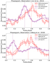 |
Fig. 3. Results of the timing checks that were performed based on the literature. The pulse profiles were obtained using the timing solutions published in Lin et al. (2013, top) and Wang et al. (2018, bottom). Both Fermi-LAT and XMM-Newton counts were normalised to 1. Statistical error bars are included for both phaseograms. The dotted vertical lines indicate the best-fit locations of the X-ray peak and higher γ-ray peak. No photon weights were applied. |
The profile obtained for the first XMM-Newton observation using the timing solution in Lin et al. (2013) shows a phase lag of 0.155 ± 0.014, which is consistent with the finding of Wang et al. (2018; cf. 0.14), as well as with the phase lag of 0.150 ± 0.016 obtained from our analysis. However, while the pulse profiles in Wang et al. (2018) indicate a ∼0.14 phase lag, the profiles from our re-analysis indicate a phase lag of 0.361 ± 0.015, which appears to be inconsistent with the finding of Wang et al. (2018) and in agreement with our full-mission and local timing analyses. A possible explanation could be related to the fact that the method based on correlations, also used by Wang et al. (2018), provides extremely large uncertainties, as shown in Sect. 3.1, and therefore cannot be considered robust enough to draw conclusions.
We also considered whether the change in phase lag that we observed could be related to drifts in the Fermi-LAT clock that might cause different γ-to-X relative phase at different epochs. However, Ajello et al. (2021) have shown that the Fermi-LAT time stamp for each photon is accurate to 300 ns in absolute time.
Finally, we addressed whether the discrepancy in phase measurements could be related to the timing accuracy in XMM-Newton (Martin-Carrillo et al. 2012). We searched for anomalous time jumps in all pn small-window observations of PSR J2021+4026, but found none, and therefore, we exclude XMM-Newton timing jumps as the cause of the phase shift.
As a final check, we performed our local timing analysis on the Crab pulsar, which has been used to evaluate the XMM-Newton timing accuracy (Martin-Carrillo et al. 2012). We report the details of this analysis in Appendix A. Our conclusion is that there is no change in phase lag between the Fermi-LAT and XMM-Newton pulses of the Crab, which confirms that the results reported in this section are unlikely to be an artefact of our analysis methods.
3.4. Multi-epoch X-ray spectroscopy
We performed a standard spectral analysis of the X-ray data of PSR J2021+4026 at the two different epochs of the XMM-Newton observations: the first analysis was made about 6 months after the first mode change, and the second one was made when the γ-ray flux had recovered to the initial state (see Table 1). We performed a standard search for high particle background periods (following De Luca et al. 2005) and excluded them, thus obtaining good exposure times of ∼80 ks and ∼95 ks for the two observations, respectively. We extracted photons within 30″ of the pulsar position, as determined by Chandra, to obtain the source spectra. Background spectra were extracted from nearby source-free regions. We extracted 0–4 pattern events for pn and 0–12 for the MOS detectors. Finally, we grouped spectra to have at least 25 counts per bin, resulting in 16 energy bins in the 0.3–12 keV range.
To fit the spectra, we used the XSPEC package v.12.10.1 (Arnaud 1996), considering events in the 0.3–10 keV energy range. We fitted the spectra of the two observations separately using either an absorbed blackbody (bbodyrad), (abundances from Wilms et al. 2000, XSPEC model tbabs) or an absorbed power law (powerlaw). Single-component models give statistically unacceptable fits, with null hypothesis probabilities (n.h.p.) < 5 × 10⁻⁵. Thus, we tried a two-component model (absorbed power law plus blackbody). For both observations, we obtained an acceptable fit with n.h.p. of 0.04 and 0.34, respectively. With the model settled, we searched for significant differences in the spectra and/or fluxes between the two observations. We found no evidence of spectral shape or flux changes. The contemporaneous fits of both spectra with all the model parameters yielded results with acceptable n.h.p. of 0.067 (reduced χ2 of 1.15 with 210 degrees of freedom). Using this model, we obtained a hydrogen absorption column density NH = (1.2 ± 0.2)×1022 cm−2, a blackbody temperature kT = (215 ± 15) eV (consistent with Lin et al. 2013), a blackbody emitting radius of 
 m (where d1.5 is the distance in units of 1.5 kpc), and a photon index Γ = 1.0 ± 0.3 (all the errors are at 1σ confidence). The unabsorbed thermal flux in the 0.3–12 keV band is (11.0 ± 2.4)×10−14 erg cm−2 s−1, and the unabsorbed non-thermal flux is (3.2 ± 0.7)×10−14 erg cm−2 s−1.
Finally, we searched for changes in the parameters of the thermal component. We performed fits using the same model as above, but with the parameters of the thermal component left free to vary between the different observations. We obtained the contour plots reported in Fig. 4 for the pairs of parameters describing the thermal emission of the two different observations, indicating consistent temperatures.
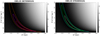 |
Fig. 4. Contour plots of the thermal model parameters for the two different XMM-Newton observations that were obtained as described in Sect. 3.4. We plot the temperature against the emitting radius. We also report the χ2 value for each realization, where the degrees of freedom are 208. We show the 1σ, 90%, and 3σ confidence level contours around the best fit (marked with a cross). |
4. Searching for an optical counterpart
We searched for the PSR J2021+4026 optical counterpart in the GTC/OSIRIS images using the Chandra coordinates reported in Weisskopf et al. (2011) as a reference, with a 99% confidence level uncertainty of 1″. Since PSR J2021+4026 is radio quiet and no multi-epoch Chandra observations are available, we could not measure its proper motion from Chandra observations, and the whitening parameters required for this young and energetic pulsar make it challenging to measure them directly from Fermi-LAT timing. For the distance of the γ Cygni SNR (1.5 ± 0.4 kpc), as determined by Landecker et al. (1980) and the average transverse pulsar velocity (400 km s−1) by Hobbs et al. (2004), we would expect an angular displacement of  in an unknown direction at the epoch of our GTC observations (MJD = 57547), which we must account for together with the nominal error on the pulsar position. We computed the astrometric solution on the GTC/OSIRIS images using the wcstools8 software package, matching the sky and pixel coordinates of stars selected from the Two Micron All Sky Survey (2MASS) All-Sky Catalog of Point Sources (Skrutskie et al. 2006), with an overall accuracy of ∼0
 2.
2.
Figure 5 shows the OSIRIS co-added g′-band image of the PSR J2021+4026 field. Although star BD+39 4152 was offset to chip 1, its scattered light is still strong enough to increase the sky background at the aim point in Chip 2 in the g′- and r′-band images by 30% and 35%, respectively. We computed the increase in sky background by sampling the counts and rms at the pulsar position in a box of 25 × 25 pixels ( ), and, in the same way, in different regions at the western part of the CCD chip at the greatest distance from BD+39 4152, where the sky background is least intense, and averaged the measurements. We computed the 3σ limiting magnitudes at the pulsar position from the rms of the sky background (Newberry 1991), obtaining r′ = 25.3 and g′ = 26.1, the deepest constraints to date on the pulsar brightness. We corrected these values for the interstellar reddening in the pulsar direction, E(B − V) = 2.15 ± 0.04, derived from the NH best-fitting the XMM-Newton X-ray spectra (see previous section) and the relation of Predehl & Schmitt (1995). We checked that this value is consistent with the Galactic extinction maps within 5′ of the location of the pulsar. For the estimated reddening value, the extinction-corrected flux upper limits at the g′- and r′-band peak frequencies are Fg′ = 3.3 × 10⁻²⁸ and Fr′ = 2.4 × 10⁻²⁸ erg cm−2 s−1 Hz−1. Figure 6 shows that the optical upper limits are below and above the extrapolations of the γ− and X-ray power-law spectral models, respectively, underlining the discontinuity in the multiwavelength spectrum, a characteristic seen in other pulsars (Mignani et al. 2018). Our g′-band upper limit corresponds to an unabsorbed flux Fg′ ≲ 6.8 × 10⁻¹⁴ erg cm−2 s−1, implying an optical luminosity Lg′ ≲ 18.3 × 1030 erg s−1
 , consistent with the values observed in pulsars of the same age as PSR J2021+4026 (Mignani et al. 2016).
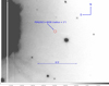 |
Fig. 5. GTC/OSIRIS zoomed g′-band image of the PSR J2021+4026 field. The pulsar position is marked by the red circle, whose radius accounts both for the absolute uncertainty on the pulsar Chandra coordinates and the accuracy of our astrometric solution. The intensity levels in the bottom bar are in ADU and have been adjusted for a better clarity. The point-spread function wings of the bright star BD+39 4152 are visible on the left, overflowing from the gap between the two CCDs. The white band on the left corresponds to the CCD gap residual after image dithering. |
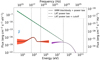 |
Fig. 6. Best-fit functions and 1σ confidence contours for the XMM and LAT spectra of PSR J2021+4026. The parameters for the XMM spectral models are those reported in Sect. 3.4. LAT spectral models are taken from the 4FGL-DR2 catalogue. Power laws were extrapolated down to 1 eV to highlight the observed discontinuity in the high-energy spectral index. The optical upper limits are reported in blue. The dotted vertical lines indicate the validity energy bands of the X-ray (0.3–12 keV) and γ-ray (0.1–300 GeV) best-fit functions. |
5. Discussion
Our multiwavelength timing monitoring observations have revealed a shift in the relative phase of the X- and γ-ray pulses between two epochs having different f1 and γ-ray flux. We can use the results based on full mission and local timing analyses reported in Sects. 3.1 and 3.2 to compute a weighted average of the phase lag, obtaining 0.21 ± 0.02. This shift could be related to the state changes undergone by the pulsar, and we present here a toy model to interpret these results.
The X-ray spectral analysis suggests that the X-ray emission could be due to polar cap heating. The blackbody + power-law fit presented in Sect. 3.4 points to a thermal emission region of radius ∼340 m and a luminosity of ∼2.5 × 1031 erg s−1, which matches the predicted polar cap heating luminosity of 1031 erg s−1 reported in Harding & Muslimov (2001) reasonably well. The measured temperature of the polar cap is higher than we would expect for a cooling neutron star with ∼77 kyr such as PSR J2021+4026 (Rigoselli et al. 2021; Potekhin et al. 2020).
The shift of the X-ray pulse phase by 0.21, if corresponding to the emission coming from one of the magnetic poles, is much larger than the size of a standard polar cap (Page et al. 2004). Here we speculate that the pulsar has a multipolar magnetic field, where the quadrupole component is dominant near the stellar surface. However, at large distances from the neutron star, this quadrupole component is not easily detectable because the dipole field will dominate and the global magnetospheric structure will be that of a dipole, with the current sheet outside the light cylinder producing the emission observed at γ-ray energies by Fermi (Kalapotharakos et al. 2014). In this configuration, the high-altitude dipole-dominated field lines will need to connect with the poles of the quadrupole-dominated field lines, depending on the strength and alignment of this component. This connection would lead to a heating of some but not all of the poles. If an event, such as the mode change observed in the pulsar, happens to change either the surface multipolar field or the configuration of the current sheet, the current sheet could connect to a different pole. We expect that the poles of a star-centred quadrupole component are about 0.25 in phase apart; therefore, this reconfiguration might explain the observed phase shift in the X-ray peak. A multipolar field has in fact been strongly inferred for the millisecond pulsar PSR J0030+0451 from fitting of its thermal X-ray profile using NICER data (Kalapotharakos et al. 2021). Quadrupole field components can produce polar caps that are larger and more extended that those of a pure dipole field (Gralla et al. 2017). Rigoselli et al. (2021), using a more complex magnetic atmosphere model to fit the X-ray profile of PSR J2021+4026, find a heated area much larger than dipole.
This model could also explain the observed variability in γ-rays. If the pole connected to the current sheet immediately after the first state change had properties more favourable to pair production (e.g. higher surface field strength, smaller field radius of the curvature), then an increase in pair multiplicity, or equivalently, in conductivity, would increase f0 (Kalapotharakos et al. 2012; Li et al. 2012b). An increase in conductivity would also decrease the accelerating electric field in the current sheet because more pairs would result in greater screening, which would decrease the γ-ray flux as observed during the mode changes in 2011 and 2014. Moreover, a decreased electric field would also lead to a lower cutoff energy. A decrease in the spectral cutoff energy was observed during the first mode change in 2011 (Allafort et al. 2013).
The number of γ-ray pulsars detected by the LAT has increased to nearly 300 since its launch9, however, PSR J2021+4026 is still the only isolated pulsar to have shown such evident mode changes. This unique behaviour is thus difficult to explain, but a combination of magnetospheric properties and viewing geometry may contribute. Ng et al. (2016) suggest that the mode changes are associated with a reconfiguration of the magnetic field on the neutron star surface due to crustal plate tectonics. Alternatively, quasi-periodic changes in the current sheet, due to changes in plasma supply to the magnetosphere (Li et al. 2012a), could cause the dipole field component to connect to different poles of the quadrupole component.
6. Conclusions
We have presented an updated multiwavelength analysis of PSR J2021+4026 emission using Fermi-LAT, XMM-Newton, and GTC data to better understand the physics behind the mode changes experienced by this pulsar in 2011 and 2014. Through a simultaneous analysis of XMM-Newton and Fermi data, we detected a shift in the relative phase between the X and γ-ray pulses. This phase shift was not observed before, and so we have performed two complementary analyses using a full mission, whitened timing solution (Sect. 3.1) and two simpler timing solutions based on short time windows centred around the two XMM-Newton observations (Sect. 3.2). Both analyses confirmed the phase shift, and they produce a consistent value of 0.21 ± 0.02 in phase.
Since the X-ray emission is consistent with that of a heated polar cap, we interpret this phase shift as a change in the connection of dipole field lines with inner quadrupole field components close to the stellar surface. We suggest that mode changes would affect the accelerating electric field, thus producing a simultaneous decrease in flux and increase in f1, as observed for the pulsar.
Furthermore, we observed PSR J2021+4026 with the 10.4 m GTC to search for an optical counterpart whose flux was possibly enhanced following the mode change, but we could not detect it down to g′ = 26.1 and r′ = 25.3. The background from star BD+39 4152 (V ∼ 8.6) at ∼1′ prevented the limits from being deeper. Observations with the Hubble Space Telescope would provide the only possibility to detect the pulsar in the optical and pave the way to coordinated multiwavelength monitoring programmes.
The repeating nature of the variability event observed for PSR J2021+4026 on timescales of a few years suggests that the pulsar magnetosphere is affected by some periodic reconfiguration. A continuous monitoring of the source would be fundamental for understanding the physics of this unique γ-ray-emitting neutron star in more detail.

Public list of LAT detected pulsars available at: https://confluence.slac.stanford.edu/display/GLAMCOG/Public+List+of+LAT-Detected+Gamma-Ray+Pulsars
Acknowledgments
The authors would like to thank the Fermi-LAT internal referee David Smith and the anonymous reviewer at the journal for their useful review and discussions which improved the manuscript. The Fermi-LAT Collaboration acknowledges generous ongoing support from a number of agencies and institutes that have supported both the development and the operation of the LAT as well as scientific data analysis. These include the National Aeronautics and Space Administration and the Department of Energy in the United States, the Commissariat à l’Energie Atomique and the Centre National de la Recherche Scientifique/Institut National de Physique Nucléaire et de Physique des Particules in France, the Agenzia Spaziale Italiana and the Istituto Nazionale di Fisica Nucleare in Italy, the Ministry of Education, Culture, Sports, Science and Technology (MEXT), High Energy Accelerator Research Organization (KEK) and Japan Aerospace Exploration Agency (JAXA) in Japan, and the K. A. Wallenberg Foundation, the Swedish Research Council and the Swedish National Space Board in Sweden. Additional support for science analysis during the operations phase is gratefully acknowledged from the Istituto Nazionale di Astrofisica in Italy and the Centre National d’Études Spatiales in France. This work performed in part under DOE Contract DE-AC02-76SF00515. Based on observations made with the Gran Telescopio Canarias (GTC), installed in the Spanish Observatorio del Roque de los Muchachos of the Instituto de Astrofísica de Canarias, in the island of La Palma. IRAF is distributed by the National Optical Astronomy Observatories, which are operated by the Association of Universities for Research in Astronomy, Inc., under cooperative agreement with the National Science Foundation. Work at NRL is supported by NASA.
References
- Abdo, A. A., Ackermann, M., Ajello, M., et al. 2009, Science, 325, 840 [Google Scholar]
- Abdo, A. A., Ackermann, M., Ajello, M., et al. 2010, ApJ, 708, 1254 [Google Scholar]
- Abdollahi, S., Acero, F., Ackermann, M., et al. 2020, ApJS, 247, 33 [Google Scholar]
- Ajello, M., Atwood, W. B., Axelsson, M., et al. 2021, ApJS, 256, 12 [NASA ADS] [CrossRef] [Google Scholar]
- Ajello, M., Atwood, W. B., Baldini, L., et al. 2022, Science, 376, 521 [NASA ADS] [CrossRef] [Google Scholar]
- Allafort, A., Baldini, L., Ballet, J., et al. 2013, ApJ, 777, L2 [NASA ADS] [CrossRef] [Google Scholar]
- Arnaud, K. A. 1996, ASP Conf. Ser., 101, 17 [Google Scholar]
- Atwood, W. B., Abdo, A. A., Ackermann, M., et al. 2009, ApJ, 697, 1071 [CrossRef] [Google Scholar]
- Atwood, W., Albert, A., Baldini, L., et al. 2013, ArXiv e-prints [arXiv:1303.3514] [Google Scholar]
- Bruel, P., Burnett, T. H., Digel, S. W., et al. 2018, ArXiv e-prints [arXiv:1810.11394] [Google Scholar]
- Collins, S., Shearer, A., & Mignani, R. 2011, AIP Conf. Ser., 1357, 310 [NASA ADS] [Google Scholar]
- Cordes, J. M., & Lazio, T. J. W. 2002, ArXiv e-prints [arXiv:astro-ph/0207156] [Google Scholar]
- de Jager, O. C., & Büsching, I. 2010, A&A, 517, L9 [NASA ADS] [CrossRef] [EDP Sciences] [Google Scholar]
- De Luca, A., Caraveo, P. A., Mereghetti, S., Negroni, M., & Bignami, G. F. 2005, ApJ, 623, 1051 [NASA ADS] [CrossRef] [Google Scholar]
- Fukugita, M., Ichikawa, T., Gunn, J. E., et al. 1996, AJ, 111, 1748 [Google Scholar]
- Gralla, S. E., Lupsasca, A., & Philippov, A. 2017, ApJ, 851, 137 [NASA ADS] [CrossRef] [Google Scholar]
- Harding, A. K., & Muslimov, A. G. 2001, ApJ, 556, 987 [NASA ADS] [CrossRef] [Google Scholar]
- Higgs, L. A., Landecker, T. L., & Roger, R. S. 1977, AJ, 82, 718 [Google Scholar]
- Hobbs, G., Lyne, A. G., Kramer, M., Martin, C. E., & Jordan, C. 2004, MNRAS, 353, 1311 [NASA ADS] [CrossRef] [Google Scholar]
- Hobbs, G. B., Edwards, R. T., & Manchester, R. N. 2006, MNRAS, 369, 655 [Google Scholar]
- Kalapotharakos, C., Harding, A. K., Kazanas, D., & Contopoulos, I. 2012, ApJ, 754, L1 [Google Scholar]
- Kalapotharakos, C., Harding, A. K., & Kazanas, D. 2014, ApJ, 793, 97 [Google Scholar]
- Kalapotharakos, C., Wadiasingh, Z., Harding, A. K., & Kazanas, D. 2021, ApJ, 907, 63 [NASA ADS] [CrossRef] [Google Scholar]
- Kaplan, D. L., Chatterjee, S., Gaensler, B. M., & Anderson, J. 2008, ApJ, 677, 1201 [NASA ADS] [CrossRef] [Google Scholar]
- Kirsch, M. G. F., Schönherr, G., Kendziorra, E., et al. 2006, A&A, 453, 173 [NASA ADS] [CrossRef] [EDP Sciences] [Google Scholar]
- Landecker, T. L., Roger, R. S., & Higgs, L. A. 1980, A&AS, 39, 133 [Google Scholar]
- Li, J., Spitkovsky, A., & Tchekhovskoy, A. 2012a, ApJ, 746, 60 [Google Scholar]
- Li, J., Spitkovsky, A., & Tchekhovskoy, A. 2012b, ApJ, 746, L24 [CrossRef] [Google Scholar]
- Lin, L. C. C., Hui, C. Y., Hu, C. P., et al. 2013, ApJ, 770, L9 [Google Scholar]
- Luo, J., Ransom, S., Demorest, P., et al. 2021, ApJ, 911, 45 [NASA ADS] [CrossRef] [Google Scholar]
- Marelli, M., Pizzocaro, D., De Luca, A., et al. 2016, ApJ, 819, 40 [NASA ADS] [CrossRef] [Google Scholar]
- Marshall, F. E., Guillemot, L., Harding, A. K., Martin, P., & Smith, D. A. 2015, ApJ, 807, L27 [NASA ADS] [CrossRef] [Google Scholar]
- Martin-Carrillo, A., Kirsch, M. G. F., Caballero, I., et al. 2012, A&A, 545, A126 [NASA ADS] [CrossRef] [EDP Sciences] [Google Scholar]
- Mignani, R. P., Rea, N., Testa, V., et al. 2016, MNRAS, 461, 4317 [NASA ADS] [CrossRef] [Google Scholar]
- Mignani, R. P., Testa, V., Rea, N., et al. 2018, MNRAS, 478, 332 [NASA ADS] [CrossRef] [Google Scholar]
- Newberry, M. V. 1991, PASP, 103, 122 [NASA ADS] [CrossRef] [Google Scholar]
- Ng, C. W., Takata, J., & Cheng, K. S. 2016, ApJ, 825, 18 [CrossRef] [Google Scholar]
- Page, D., Lattimer, J. M., Prakash, M., & Steiner, A. W. 2004, ApJS, 155, 623 [NASA ADS] [CrossRef] [Google Scholar]
- Potekhin, A. Y., Zyuzin, D. A., Yakovlev, D. G., Beznogov, M. V., & Shibanov, Y. A. 2020, MNRAS, 496, 5052 [NASA ADS] [CrossRef] [Google Scholar]
- Predehl, P., & Schmitt, J. H. M. M. 1995, A&A, 500, 459 [Google Scholar]
- Ray, P. S., Kerr, M., Parent, D., et al. 2011, ApJS, 194, 17 [NASA ADS] [CrossRef] [Google Scholar]
- Rigoselli, M., Mereghetti, S., Taverna, R., Turolla, R., & De Grandis, D. 2021, A&A, 646, A117 [NASA ADS] [CrossRef] [EDP Sciences] [Google Scholar]
- Skrutskie, M. F., Cutri, R. M., Stiening, R., et al. 2006, AJ, 131, 1163 [NASA ADS] [CrossRef] [Google Scholar]
- Smith, J. A., Tucker, D. L., Kent, S., et al. 2002, AJ, 123, 2121 [NASA ADS] [CrossRef] [Google Scholar]
- Takata, J., Wang, H. H., Lin, L. C. C., et al. 2020, ApJ, 890, 16 [NASA ADS] [CrossRef] [Google Scholar]
- Wang, H. H., Takata, J., Hu, C. P., Lin, L. C. C., & Zhao, J. 2018, ApJ, 856, 98 [NASA ADS] [CrossRef] [Google Scholar]
- Weisskopf, M. C., Romani, R. W., Razzano, M., et al. 2011, ApJ, 743, 74 [NASA ADS] [CrossRef] [Google Scholar]
- Wilms, J., Allen, A., & McCray, R. 2000, ApJ, 542, 914 [Google Scholar]
- Zhao, J., Ng, C. W., Lin, L. C. C., et al. 2017, ApJ, 842, 53 [NASA ADS] [CrossRef] [Google Scholar]
Appendix A: Timing checks using the Crab pulsar
To validate our local timing analysis, we applied it to observations of the Crab pulsar. This source is frequently observed by XMM-Newton to check for any timing inaccuracies (Martin-Carrillo et al. 2012). Its sharp peaks allow a precise measurement of the γ- and X-ray phase lag, which has been observed to remain steady with time (Kirsch et al. 2006; Abdo et al. 2010).
We produced three clean event files using the XMM-Newton calibration observations performed periodically on the Crab. The first 7.4 ks observation (Obs ID 0611181301, PI Jansen, hereafter observation 1) was performed on 2012 February 23 (MJD 55981). The second (Obs ID 0611182801, PI Jansen, hereafter observation 2) was performed on 2015 August 29 (MJD 57263). The third (Obs ID 0611183201, PI Jansen, hereafter observation 3) was performed on 2016 February 24 (MJD 57442) and lasted 2.9 ks. We selected events from the pn Camera in timing mode, and we barycentered using the barycen tool adopting the pulsar position  ;
;  (Kaplan et al. 2008) and using the DE405 ephemerides.
We then applied the local timing analysis described in Section 3.2 to these three observations and fitted the phaseograms with PINT (Luo et al. 2021) using two Gaussian peaks in order to evaluate the phase lag between the γ-ray and X-ray pulse profile, shown in Fig. A.1. For viewing purposes, we applied a phase offset so that the first peak of the X-ray curve was always located at phase 0.3. Therefore, this example is also useful to illustrate how we define ϕ0 according to Equation 1 and how this does not affect the relative phase difference between X and γ phaseograms. The phase lag between the γ and X-ray phaseograms for the three XMM-Newton observations of the Crab is 0.007 (0.0076±0.0018 for observation 1, 0.0066±0.0012 for observation 2, and 0.0063±0.0018 for observation 3), meaning that the γ-to-X-ray pulse profile alignment is stable, in agreement with our expectations.
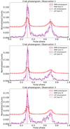 |
Fig. A.1. Results of the timing check made using three XMM-Newton observations of the Crab pulsar. Fermi counts were normalized to 1, and XMM-Newton counts were normalized to 3 for display purposes. Statistical error bars are included for both phaseograms. The potted vertical lines indicate the best-fit locations of the X-ray peak and higher γ-ray peak. No photon weights were applied. |
All Tables
Parameters and results of the local timing test for the two XMM-Newton observations discussed in Lin et al. (2013, Obs. 1) and Wang et al. (2018, Obs. 2).
All Figures
|
Fig. 1. Results from the full-mission timing analysis using best fits to the pulse profiles as described in Sect. 3.1. The top and bottom plots refer to the first and second XMM-Newton observations, respectively. Fermi-LAT counts were calculated using photon weights. XMM-Newton counts were normalized to 1, while Fermi-LAT counts were normalized to 2 for display purposes. Counts from the diffuse γ-ray background are not shown. Statistical error bars are included for both phaseograms. The dotted vertical lines indicate the best-fit locations of the X-ray peak and higher γ-ray peak. |
| In the text | |
|
Fig. 2. Results from the local timing analysis described in Sect. 3.2. The top and bottom plots refer to the first and second XMM-Newton observations, respectively. Fermi-LAT counts were calculated using photon weights. Both Fermi-LAT and XMM-Newton counts were normalised to 1. Counts from the diffuse γ-ray background are not shown. Statistical error bars are included for both phaseograms. The dotted vertical lines indicate the best-fit locations of the X-ray peaks and higher γ-ray peaks. An initial phase ϕ0 = −0.19 was introduced in the first observation mostly for display purposes in order to align the γ-ray phaseogram with that of the second observation. |
| In the text | |
|
Fig. 3. Results of the timing checks that were performed based on the literature. The pulse profiles were obtained using the timing solutions published in Lin et al. (2013, top) and Wang et al. (2018, bottom). Both Fermi-LAT and XMM-Newton counts were normalised to 1. Statistical error bars are included for both phaseograms. The dotted vertical lines indicate the best-fit locations of the X-ray peak and higher γ-ray peak. No photon weights were applied. |
| In the text | |
|
Fig. 4. Contour plots of the thermal model parameters for the two different XMM-Newton observations that were obtained as described in Sect. 3.4. We plot the temperature against the emitting radius. We also report the χ2 value for each realization, where the degrees of freedom are 208. We show the 1σ, 90%, and 3σ confidence level contours around the best fit (marked with a cross). |
| In the text | |
|
Fig. 5. GTC/OSIRIS zoomed g′-band image of the PSR J2021+4026 field. The pulsar position is marked by the red circle, whose radius accounts both for the absolute uncertainty on the pulsar Chandra coordinates and the accuracy of our astrometric solution. The intensity levels in the bottom bar are in ADU and have been adjusted for a better clarity. The point-spread function wings of the bright star BD+39 4152 are visible on the left, overflowing from the gap between the two CCDs. The white band on the left corresponds to the CCD gap residual after image dithering. |
| In the text | |
|
Fig. 6. Best-fit functions and 1σ confidence contours for the XMM and LAT spectra of PSR J2021+4026. The parameters for the XMM spectral models are those reported in Sect. 3.4. LAT spectral models are taken from the 4FGL-DR2 catalogue. Power laws were extrapolated down to 1 eV to highlight the observed discontinuity in the high-energy spectral index. The optical upper limits are reported in blue. The dotted vertical lines indicate the validity energy bands of the X-ray (0.3–12 keV) and γ-ray (0.1–300 GeV) best-fit functions. |
| In the text | |
|
Fig. A.1. Results of the timing check made using three XMM-Newton observations of the Crab pulsar. Fermi counts were normalized to 1, and XMM-Newton counts were normalized to 3 for display purposes. Statistical error bars are included for both phaseograms. The potted vertical lines indicate the best-fit locations of the X-ray peak and higher γ-ray peak. No photon weights were applied. |
| In the text | |
Current usage metrics show cumulative count of Article Views (full-text article views including HTML views, PDF and ePub downloads, according to the available data) and Abstracts Views on Vision4Press platform.
Data correspond to usage on the plateform after 2015. The current usage metrics is available 48-96 hours after online publication and is updated daily on week days.
Initial download of the metrics may take a while.