| Issue |
A&A
Volume 685, May 2024
|
|
|---|---|---|
| Article Number | A144 | |
| Number of page(s) | 15 | |
| Section | Atomic, molecular, and nuclear data | |
| DOI | https://doi.org/10.1051/0004-6361/202348473 | |
| Published online | 20 May 2024 | |
Electronic structure, oscillator strength, and rovibrationally resolved photodissociation of 24MgH
1
School of Physics and Information Technology, Shaanxi Normal University, Xi'an 710119, PR China
e-mail: This email address is being protected from spambots. You need JavaScript enabled to view it.
; This email address is being protected from spambots. You need JavaScript enabled to view it.
2
School of Physics, Henan Normal University, Henan 453000, PR China
3
College of Physics, Jilin University, Jilin 130012, PR China
4
Institute of Applied Physics and Computational Mathematics, Beijing 100088, PR China
5
Center for Applied Physics and Technology, Peking University, Beijing 100084, PR China
Received:
2
November
2023
Accepted:
17
February
2024
Abstract
Aims. A series of high-precision calculations for the electronic structure of MgH have been reported in the past two decades; however, most of them d not include the core-valence correlation and still exhibit distinct differences. Furthermore, the latest high-precision results have not been applied to the studies of photodissociation dynamics. The primary motivations of this paper are to calculate a more precise electronic structure of MgH consering a core-valence correlation and to prove the photodissociation cross-sections.
Methods. The electronic structure of MgH is investigated by multi-reference configuration interaction calculations with Davson correction (MRCI+Q). We performed two different sets of calculations to investigate the core-valence correlation and, as a result, obtained accurate potential energy curves (PECs) and transition dipole moments (TDMs). An extrapolation procedure was also employed to eliminate the error of basis set. Then, the photodissociation cross-sections were calculated using high-precision PECs and TDMs.
Results. The PECs and TDMs of the five lowest doublet electronic states, X2Σ+, B′2Σ+, E2Σ+, A2Π, and C2Π, are obtained from calculations including core-valence correlation, termed as CV-MRCI, while PECs of the ten lowest doublet states and three quartet states are also obtained from NCV-MRCI calculations without core-valence correlation. The spectroscopic constants and band oscillator strengths are also proved with high precision levels. The equilibrium Re and vertical excitation energy Te are only 0.1% different from the measurements. Based on the CV-MRCI results, the rovibrationally resolved photodissociation cross-sections for transitions from X2Σ+ to the other four states, as well as the total local thermodynamic equilibrium cross-sections for temperatures up to 10000 K, are calculated.
Key words: atomic data / molecular processes / stars: atmospheres / galaxies: abundances
© The Authors 2024
 Open Access article, published by EDP Sciences, under the terms of the Creative Commons Attribution License (https://creativecommons.org/licenses/by/4.0), which permits unrestricted use, distribution, and reproduction in any medium, provided the original work is properly cited.
This article is published in open access under the Subscribe to Open model. This email address is being protected from spambots. You need JavaScript enabled to view it. to support open access publication.
1 Introduction
The investigation of magnesium hydride has attained considerable interest in modern research owing to its prevalence within interstellar gas and stars. MgH has been observed not only in the Sun (Lambert et al. 1971), but also within the atmospheres of numerous cool stars (Weck et al. 2003a). Along with other metallic diatomic molecules, 24MgH serves as an indicator of the isotopic abundance of magnesium in cool dwarfs, giants, and super-metal-rich stars (McWilliam & Lambert 1988; Barbuy 1987). The study of electronic structure and various dynamic processes plays a fundamental role in the research into the formation, destruction, and concentration of MgH. Photodissociation is one such process, and it significantly influences stellar atmospheric models, as it serves as an important source in the opacity at visible and UV wavelengths (Weck et al. 2003b). Furthermore, the photodissociation of MgH can also be employed to find the gravity of Arcturus (Bell et al. 1985).
A number of recent studies have considered the photodissociation of various molecules (Qin et al. 2022, 2021), since the great improvement of computational capabilities facilitates highly accurate descriptions of molecular structure and dynamics. However, research into the photodissociation of MgH is very limited. In the work of Kirby et al. (1979); Bhattacharyya & Basu (1983); Datta et al. (1983), photodissociation cross-sections were calculated from the v″= 0 level of ground state X2∑+ through the B′2∑+ state. In recent studies (Weck et al. 2003a,a), partial cross-sections were evaluated for B′2∑+ ← X2∑+ and A2Π ← X2∑+ transitions for 313 rovibrational levels of the ground state. The potential energy curves (PECs) and transition dipole moment (TDMs) adopted in these works are the results of Saxon et al. (1978), where the three outermost electrons of MgH are allowed to distribute in the valence and virtual orbitals in STDCI calculation with a slater-type basis set. Meanwhile, in order to optimize the calculation of photodissociation cross-sections, Weck et al. (2003b,a) adjusted the PECs of Saxon et al. (1978) to coincide with experimental values.
In the past two decades, more precise methodologies have been employed in structure calculations of MgH. For instance, the MRCI method with a very large basis set (Mestdagh et al. 2009; Guitou et al. 2010; Mostafanejad & Shayesteh 2012; Chattopadhyaya 2016; El-Kork et al. 2018) has been employed to compute the PECs of MgH. The outcomes of these efforts offer substantially higher levels of precision in the electronic structure. However, most of these calculations did not include core-valence correlation and still exhibit distinct differences in both PECs and TDMs, as one can see in Figs. 1 and 2. Furthermore, these high-precision structures have not been applied to the study of photodissociation dynamics.
The motivation of present research is to investigate accurate electronic structures of MgH and then provide high-precision photodissociation cross-sections. The PECs of the ten lowest doublet states and three quartet states are obtained via multi-reference configuration interaction calculations with a Davidson correction (Langhoff & Davidson 1974) (MRCI+Q). Since our focus on the photodissociation dynamics from the ground state X2∑+ to the low-lying electronic excited states, a more accurate calculation including core-valence correlation has been performed for the PECs and TDMs of the ground X2∑+ and the four lowest doublet-excited states, B′2∑+, E2∑+, A2Π, and C2Π. The spectroscopic constants and band oscillator strengths are also provided as a further check. Then, the rovibrationally resolved photodissociation cross-sections and total photodissociation cross-sections for temperatures up to 10 000 K, with a local thermodynamic equilibrium (LTE) assumption, are obtained and reported.
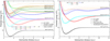 |
Fig. 1 Potential energy curves. (a) Solid lines: NCV-MRCI results. Dashed lines: CV-MRCI results. Dotted lines: Mestdagh et al. (2009). Dashed-dotted lines: El-Kork et al. (2018). Triangles: Guitou et al. (2010). (b) Solid lines: NCV-MRCI results. Dashed lines: CV-MRCI results. Dotted lines: Saxon et al. (1978). Dashed-dotted lines: Chattopadhyaya (2016). Triangles: Mostafanejad & Shayesteh (2012). |
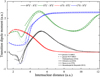 |
Fig. 2 Transition dipole moments of B′2∑+–X2∑+, A2Π–X2∑+, C2π–X2∑+ and E2∑+–X2∑+ for MgH. Solid lines: CV-MRCI calculations. Dashed lines: NCV-MRCI calculations. Dotted lines: Chattopadhyaya (2016). Solid lines with stars: El-Kork et al. (2018). Solid lines with triangles: Saxon et al. (1978). Solid lines with circles: Mostafanejad & Shayesteh (2012). |
2 Theory
2.1 Electronic structure
Calculations of PECs and TDMs are performed using a quantum chemistry package, MOLPRO 2012.1 (Werner et al. 2012). In this process, a diatomic molecule with C∞v symmetry is replaced with C2v symmetry. The relations between these two point groups are ∑+=A1, Π =B1+B2, ∆=A1+A2, and ∑−=A2. In the first step, a restricted open-shell Hartree–Fock calculation (Lindh et al. 1991) is carried out to obtain initial orbitals in the state-averaged, complete-active-space self-consistent field (SA-CASSCF; Werner & Knowles 1985; Knowles & Werner 1985). The multi-configuration wave functions can then be derived from the SA-CASSCF process by optimizing both the coefficients of configurations and the basis functions simultaneously. The 1s22s22p6 electrons of Mg are placed in a closed shell, and the three outermost electrons Mg(3s2) and H(1s) are placed in the active space. Furthermore, by adopting the optimized molecular orbitals, the internally contracted MRCI+Q (Werner & Knowles 1988; Knowles & Werner 1988, 1992) are employed to calculate the single-point energies of all electronic states.
Firstly, the PECs for electronic states with dissociation limits up to the atomic configurations Mg(3s3d 1D)+H(1s 2S) are obtained in our NCV-MRCI calculations without core-valence correlation, where the basis set Aug-cc-pV5Z is used and the core-valence correlation is omitted. The active space consists of 17 orbitals (11σ, 5π, 1δ). After that, since our primary concern is the photodissociation to some low-lying electronic excited states, a more accurate calculation, termed as CV-MRCI, with core-valence correlation, is performed for the PECs and TDMs of X2∑+ and the four lowest doublet excited states, B′2∑+, E2∑+, A2Π, and C2Π, with an active space of 11 orbitals (7σ, 3π, 1δ). Two prescriptions are introduced to improve the accuracy in CV-MRCI. The Aug-cc-pWCVnZ (n = 3, 4, 5) basis sets (in the scheme of Dunning 1989; Woon & Dunning 1993; Wilson et al. 1999) are used, and the core–valence correlation of 2p6 electrons of Mg is taken into account. Then, an extrapolation procedure, based on the CV-MRCI results using the basis sets Aug-cc-pWCVnZ (n = 3, 4, 5) for both Mg and H atoms, is carried out to reach the complete basis set (CBS) limit of the PECs and TDMs by using the following formula (Müller 2006):
 (1)
(1)
where V(n) is the result calculated using Aug-cc-pWCVnZ. VCBS and the coefficients α and β are determined from a fitting procedure.
The PECs and TDMs are obtained as a function of internu-clear distance varying from 1.5 to 12.4 a.u. For bond separations beyond this, an extrapolation procedure is employed. The long-range behavior of PECs from 12.4 to 40 a.u. is approximated using the following formula:
 (2)
(2)
where C5 is the fitting parameter and  (London 1937). Γ is the ionization energy of corresponding atomic state obtained from NIST Atomic Spectra Database (Kramida et al. 2022). a represents the static dipole polarizability collected from the CCSD(T) calculations of Wang et al. (2021), where αH = 4.4962 a.u. and αMg = 70.76 a.u. are adopted. For the short-range behavior of PECs, we utilize the formula V(R) = Ae−BR + C to extend to 0.5 a.u. Here, A, B, and C are fitting coefficients. The treatment of long-range and short-range behavior in the TDMs is carried out in a similar way.
2.2 Spectroscopic constants
To obtain the spectroscopic constants, the Murrell–Sorbie (M–S) function (Murrell 1984) with n = 10 was employed in the present study to fit the PECs:
 (3)
(3)
where ρ = R − Re and Re is the equilibrium position.
By examining the relationship between parameters αi and the spectroscopic constants (Zhu 2007), these constants are derived from the formulas:
 (4)
(4)
 (5)
(5)
 (6)
(6)
 (7)
(7)
 (8)
(8)
 (9)
(9)
 (10)
(10)
where h is the Planck constant, c is the speed of light, and μ is the reduced mass with the value of 0.967184984 AMU.
The quality of fitting can be assessed by the root-mean-square error (RMSE) and the correlation coefficient (RC):
 (11)
(11)
 (12)
(12)
where N is the number of grid points. A smaller RMSE value closer to zero and an RC value closer to one indicate a good fit of the M–S function. As depicted in Table 1, the fitting is exceptionally robust, thus indicating utmost precision in the computation of spectroscopic constants.
Quality of fitting by Murrell-Sorbie Function.
2.3 Band oscillator strength
The formula for band oscillator strength was collected from Kirby et al. (1979):
 (13)
(13)
where ∆E is the transition energy and Dfi(R) is the TDM between the initial and final electronic state. χv″J″ and χv′J′ are solutions of the radial Schrödinger equation for nuclear motion on the initial and final potential curves, with J″ = 0 and J′ = 1, respectively. These were obtained numerically using the method in Yang et al. (2020). The degeneracy factor 𝑔 can be expressed as
 (14)
(14)
Λ is the projection of angular momentum along the diatomic molecule axis. In the case of the ∑ ← ∑ transition, Λ′ = 0 and Λ″ = 0, so 𝑔 = 1. For the Π ← ∑ transition, 𝑔 = 2. We note that based on the data set of oscillator strengths presented in this work, one can also obtain the corresponding Einstein A coefficients and photoabsorption cross-sections using the formulas in Bernath (2020).
2.4 Photodissociation cross-section
The formulas of photodissociation cross-section (Kirby et al. 1989; Miyake et al. 2011; Yang et al. 2020) by absorption from rovibrational level v″J″ at a photon energy Eph, are written as
 (15)
(15)
ϵ′ is the relative kinetic released energy, and the matrix element of TDM between rovibrational v″J″ of the initial bound state i and the ϵ′J′ of the final continuum state f is
 (16)
(16)
The Hönl-London factors SJ′ (J″) for ∑ ← ∑ transition, defined by Watson (2008), are
 (17)
(17)
For the Π ← ∑ transition,
 (18)
(18)
If the density of environment is sufficiently high, the population of rovibrational states is assumed to follow the Boltzmann distribution, and, as a consequence, the overall photodissociation cross-section (i.e., the so-called LTE cross-section) is dependent upon both temperature (T) and wavelength (λ) (Argyros 1974):
 (19)
(19)
where
 (20)
(20)
kB here is the Boltzmann constant.
3 Results and discussion
3.1 The PECs and TDMs
Accurate prediction of electronic structure is a solid foundation for the study of molecular dynamics. The PECs of the ten lowest doublet and three quartet electronic states of MgH, with the dissociation limits up to the atomic configurations Mg(3s3d 1D)+H(1s 2S), are obtained in the present NCV-MRCI calculations and plotted in Fig. 1. Subsequently, in order to provide dissociation cross-sections for concerned states more precisely, the PECs and TDMs of the five lowest doublet electronic states (X2∑, B′2∑+, E2∑+, A2Π and C2Π) are determined via CV-MRCI calculations and shown in Figs. 1 and 2, respectively. The PECs from Saxon et al. (1978); Mestdagh et al. (2009); Guitou et al. (2010); Mostafanejad & Shayesteh (2012); Chattopadhyaya (2016); El-Kork et al. (2018) are also displayed in Fig. 1 for comparison. For clarity, the results of Mestdagh et al. (2009); Guitou et al. (2010); El-Kork et al. (2018) are provided in Fig. 1a, while the other sets of data are shown in Fig. 1b since they are restricted to the electronic states with dissociation limits associated with Mg(3s2) + H(1s) or Mg(3s3p) + H(1s). A complete data set of the present PECs and TDMs is given in Tables A.5 and A.6.
An overall good agreement can be observed in the shapes of PECs in Fig. 1. Parallel spin of three electrons prevents the formation of any chemical bond and is responsible for the repulsive nature of the quarter states. The double-well structure in the excited 2∑+ states is a typical characteristic of alkaline-earth monohydrides (Boutalib et al. 1992; Leininger & Jeung 1995; Kerkines & Mavridis 2007). This feature arises from the fact that those states are close to each other; two of them that avoided crossings related to the upper and lower 2∑+ states, respectively, appear in the curve. This also explains the single-well structure of the B′2∑+ state since it has a relatively larger energy spacing than other 2∑+ states.
Meanwhile, given that it is consistent in the shape, obvious discrepancies still exist in the depth of potential well and dissociation limits. These calculations are mostly performed in the framework of MRCI methodology. The level of accuracy stems from the choice of the base set, the size of the active space, and the treatment of higher order effects such as spin-orbital coupling and core-valence correlation. Up to now, most works have included neither the spin-orbital coupling nor the core-valence correlation. Due to the limitation of computation capabilities, the PECs and TDMs of X2∑+, B′2∑+, and A2Π were investigated by Saxon et al. (1978) using a Slater-type basis, and they exhibit noticeably different behavior. The calculations of Guitou et al. (2010) are almost indistinguishable from present NCV-MRCI results in Fig. 1a. The only exception lies in the well of 62∑+, which is probably due to the absence of higher 2∑+ states in our calculations. Similarly, the results of X2∑+, B′2∑+, and A2Π states of Mostafanejad & Shayesteh (2012) also agree well with NCV-MRCI PECs, as shown in Fig. 1b. El-Kork et al. (2018) performed very extensive MRCI+Q calculations for the 17 lowest doublet states and 13 quarter states of MgH. The PECs correlating to the atomic levels of 3s2 1S and 3s3p 3P of Mg show an excellent agreement with the NCV-MRCI results, and they are slightly higher for the states correlating to 3s3p 1P of Mg. However, for higher excited states, the results of El-Kork et al. (2018) differ from all other calculations significantly.
The spin-orbital coupling is found to have a marginal impact on the electronic structure of MgH, as illustrated in the investigations of Chattopadhyaya (2016). On the other hand, the core-valence correlation, especially the 2p6 electrons, are expected to play an important role in the low-lying electronic states of MgH. The comparison between our NCV-MRCI and CV-MRCI results in Fig. 1b reveals that the inclusion of a core-valence correlation could induce a remarkable increase in the energies of states correlating to the two lowest asymptotic atomic levels, while the influence is lesser for states relating to 3s3p 1P of Mg and negligible for higher excited states. This effect is also included in Mestdagh et al. (2009), where a pseudopotential description of the 1s22s22p6 core, complemented by a core polarization operator, is used. Apparently, the PECs of Mestdagh et al. (2009) are slightly higher in Fig. 1a, showing a similar effect to our calculations. Actually, their PECs agree perfectly with our CV-MRCI results, although they are omitted from Fig.1 b for clarity. The calculations of Chattopadhyaya (2016) were performed with the 2s22p63s2 electrons of Mg kept in the valence region and the 1s2 core electrons described by an effective potential, based on the perturbative correction and energy extrapolation technique using the Table-direct-CI version of the MRDCI code (Krebs & Buenker 1995). However, the PECs of Chattopadhyaya (2016) in Fig. 1b are obviously higher than all other results, and the core-valence correlation seems to be overestimated.
Although there have been numbers of investigations into the PECs of MgH, studies of the TDMs are surprisingly scarce. TDMs from X2∑+ to the lowest four excited doublet states (B′2∑+, E2∑+, A2Π, and C2Π) are illustrated in Fig. 2 and compared with the findings of Saxon et al. (1978), Mostafanejad & Shayesteh (2012), Chattopadhyaya (2016), and El-Kork et al. (2018). Similarly to the case of PECs, discrepancies are evident, with notable disparities observed in the results of Saxon et al. (1978), particularly in the B′2∑+ ← X2∑+ transition at smaller internuclear distances. This discrepancy could have a substantial impact on the accuracy of corresponding photodissociation cross-sections. Consequently, there is an imperative need for updated research on the photodissociation of MgH.
Lowest dissociation limits of MgH.
3.2 Dissociation limits and spectroscopic constants
The dissociation limits and spectroscopic constants can provide a rigorous test for the predicted electronic structure since these data can be determined from experimental measurement with high levels of precision. The dissociation limits are listed in Table 2 along with the calculations mentioned above.
For the states correlating to the atomic levels of 3s3p 3P and 3s3p 1P of Mg, the present CV-MRCI calculations show the best agreement with the NIST data with differences of only 1 cm−1 and 46 cm−1, respectively. Mestdagh et al. (2009) and Chattopadhyaya (2016) also exhibit better agreement and the differences are approximately 200 cm−1. Since the core-valence correlation is also taken into account in both calculations, the discrepancies are possibly due to the completeness of the basis set that has been compensated by an extrapolation procedure in the present CV-MRCI. Given that the differences with regard to NIST data of all the remaining calculations are at a level of 1000 cm−1 for 3s3p 3P and a few hundreds cm−1 for 3s3p 1P, the good performance of the present CV-MRCI and the results of Mestdagh et al. (2009); Chattopadhyaya (2016) validate the importance of core-valence correlation. For higher excited states, except for the fact that El-Kork et al. (2018) gave significantly larger asymptotic energies, all the calculations agree well with each other, which indicates a small influence of core-valence correlation, and the disagreement with NIST data should be attributed to the completeness of basis set and active space.
The spectroscopic constants (equilibrium point Re, dissociation energy De, vibrational constants ωe and ωeχe, rotational constant Be, vibration-rotation interaction constant αe, and vertical excitation energy Te or T0) are listed in Tables A.1 and A.2 and are compared with available information. The inclusion of the core-valence correlation effect provides an obvious improvement, and the present CV-MRCI results exhibit the best agreement with experimental data (Shayesteh et al. 2004, 2007; Shayesteh & Bernath 2011), indicating a higher level of accuracy in the computation of electronic structures. Generally, the agreement level of Re and Te is approximately 1% for NCV-MRCI and 0.1% for CV-MRCI for all the states. For other constants, the agreement level varies with different states, and the present results generally show the best performance where the difference with measurements are mostly within 5%.
3.3 Band oscillator strength
Light absorption for a bound-bound transition is patently an important dynamic process; for example, rotation-vibration bands of molecules can contribute significantly to the infrared opacity in cool stellar atmospheres. The band oscillator strength is also an ideal verification of the validity of electronic structure, and it can be used to obtain the corresponding light absorption cross-section directly. The present CV-MRCI band oscillator strengths and transition energies of B′2∑+ ← X2∑+ and A2Π ← X2∑+ are listed in Table A.3 along with the data of Kirby et al. (1979). The data of B′2∑+ ← X2∑+ coincide with the result of Kirby et al. (1979), maintaining consistency in terms of the order of magnitude. Skory et al. (2003) highlighted the weak nature of the 0–0 band, which is attributable to the transition dipole moment nearing zero around the equilibrium of the ground state. While the overall trend of A2Π ← X2∑+ band oscillator strengths agrees with Kirby’s findings, notable discrepancies in magnitude emerge for v′ = 3, 4, 5, and 6. These deviations could be traced back to more accurate calculations of PECs and TDMs. Evidently, the band oscillator strengths of A2Π ← X2∑+ significantly overshadow that of the B′2∑+ ← X2∑+. A primary factor for this is the substantially larger TDM of A2Π ← X2∑+ around 3.26 a.u. compared to B′2∑+ ← X2∑+’s, meaning that the B′ ← X band system has never been seen in absorption. Incidentally, the difference in transition energy between our results and those of Kirby et al. (1979) is almost negligible (less than a hundredth of a percent). The band oscillator strengths and transition energies of the C2Π ← X2∑+ and E2∑+ ← X2∑+ channels for transitions between the vibrational number v″ = 0–3 and v′ = 0–9 are also provided in Table A.4.
3.4 Photodissociation of B′2∑+ ← X2∑+
Rovibrationally resolved photodissociation cross-sections σv″J″ have been computed from 315 rovibrational levels (v″J″) of X2∑+ and the complete data set are provided in the supplementary material. A selection of the partial cross sections of B′2∑+ ← X2∑+ transition are presented in Figs. 3–6. Following the methodology proposed by Weck et al. (2003b) and Skory et al. (2003) and utilizing the same PECs and TDMs, we effectively reproduced the photodissociation cross-sections for the transitions from the ground rovibrational levels (v″, J″) = (0,0) and (0, 18), as depicted in Fig.3. The results labeled as This Work (Reproduction) are nearly identical to those of Weck et al. (2003a), confirming the validity of our computational program. The present cross-sections, employing the PECs and TDMs calculated from the CV-MRCI and NCV-MRCI calculations, respectively, are also shown in Fig. 3. The present CV-MRCI and NCV-MRCI results are very similar. The disparity predominantly lies in the peak positions, stemming from the upward shift of the B′2∑+ state due to core-valence corrections. Contrastingly, a calculation of Weck et al. (2003b) exhibits significantly different cross-sections with a much lower magnitude and different peak position. The peak magnitude is 1.555 × 10⁻¹⁸ cm2 at 4.20 eV (2952 Å) for CV-MRCI cross-sections and 1.572 × 10⁻¹⁸ cm2 at 4.14 eV (2995 Å) for the NCV-MRCI results, while it is 0.346 × 10⁻¹⁸ cm2 at 4.25 eV (2917 Å) for those of Weck et al. (2003b). The origin of the discrepancy lies in the fact that the TDM of Saxon et al. (1978) at 1.5–3.5 a.u. shows a distinctly different trend. A further test performed by us using the TDM from Mostafanejad & Shayesteh (2012) and present CV-MRCI PECs is also performed to explore the difference. The test shows a peak of 1.718 × 10⁻¹⁸ cm2 at 4.17 eV (2973 Å), which is close to the present results. Remarkably, the variations in the TDMs within the range of smaller internuclear distances have a significant impact on the cross-section.
Figure 4 presents the cross-sections from J″ = 0 and ν″ = 0–11 of X2Σ+, demonstrating a similar trend but significant differences in the peak positions and magnitude compared to Weck et al. (2003b). The most notable behavior is that the existence of the maximum in the vicinity of 2950 Å and a local minimum around 3350 Å is almost irrelevant to the vibrational quantum number. This is probably due to fact that the TDM of B′2Σ+ ← X2Σ+ reaches zero at a certain internuclear distance. Other nodes and antinodes beyond the 2800–3400 Å range originate from the oscillating behavior of final continuum wave functions and the cutoffs represent the threshold energies. The magnitudes of local maximums of the cross-sections vary with different ν″ and basically exhibit the highest value when ν″ = 3; consequently, the peak magnitude decreases as ν″ increases when transitions only occur from levels of ν″ > 3. The only exception lies in the highest peak where the largest magnitude occurs for ν″ = 2, which is different to Weck et al. (2003b) where the cross sections with ν″ = 3 is the largest.
Furthermore, the photodissociation cross sections from ν″ = 0 with J″ = 0, 5, 10, 20, 35, 40, 44, and ν″ = 4 with J″ = 0, 20, 28, 32 are illustrated in Figs. 5 and 6, respectively. It can be found that the local maximum near 2930 Å and that near 3350 Å remain nearly unchanged with variations of vibrational and rotational quantum numbers. In Fig. 5, the cross-sections from the rovibrational levels with small J″ are close to each other, while the difference is more obvious for larger J″, which can also be found in Fig. 6. This is reasonable since the energy spacing between rotational levels increases as J″ increases. Another notable feature in both figures is the appearance of shape resonance near the thresholds in cross-sections from the rovibrational levels with higher J″. These sharp resonance structures are attributed to the existence of a large centrifugal term resulting in a barrier followed by the formation of quasi-bound state below the barrier, while the quasi-bound states slightly above the barrier are responsible for the broad resonances. These phenomena are also observed in the study of Weck et al. (2003b) where remarkable differences can be found in the magnitude and peak positions of the cross sections.
Finally, by assuming a local thermodynamic equilibrium condition and based on rovibrationally resolved cross-sections, we are able to provide the LTE cross-sections ranging from 0 K to 10 000 K with a step-size of 1000 K in Fig. 7. Consistently with what is stated above, the largest peaks are located around 2950 Å. In the vicinity of this maximum, the LTE cross-sections decrease as the temperature increases, while the trend is indeed reversed in the range beyond 2900 and 3100 Å. This feature is different in Weck et al. (2003b), where the magnitudes of all the peaks increase as the temperature increases. This variation can be explained by the populations on the rovibrational levels at different temperatures. According to the Boltzmann distribution, the molecules are assumed to be completely populated at (ν″ = 0, J″ = 0) of the ground electronic state at 0 K, and populations on higher excited levels increase with rising temperature. As illustrated in Fig. 4, the partial cross-sections with ν″ < 5 are larger than those of ν″ = 0, while in Fig. 5 the cross-sections decrease as J″ increases. Therefore, there is a competition as temperature increases. In the 2900–3100 Å range, as the temperature increases, the decrease of the cross-sections due to the increase of J″ is dominant, leading to a decline in LTE cross-sections. On the other hand, in partial cross-sections with ν″ = 0, J″ = 0 is small beyond this region. The increase in levels with larger ν″ can compensate the decrease from levels with higher J″. In fact, our calculation shows that the local maximum around 2450 Å does not always increase with rising temperature: it has a minimum at about 200 K. Within the wavelength range above 3300 Å, there are numerous small oscillatory structures, especially a prominent peak at 4260 Å. The primary contribution to this peak arises from shape resonance near the threshold, which is predominantly associated with levels that have relatively large rotational quantum numbers.
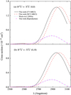 |
Fig. 3 Photodissociation cross-sections from X2∑+ to B′2∑+. (a) (v″, J″) = (0, 0) and (b) (v″, J″) = (0, 18). |
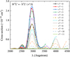 |
Fig. 4 Photodissociation cross-sections from J″ = 0 and v″ = 0–11 of x2∑+ to B′2∑+. |
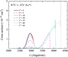 |
Fig. 5 Photodissociation cross-sections from v″ = 0 and J″ = 0, 5, 10, 20, 35, 40, 44 of X2∑+ to B′2∑+. |
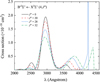 |
Fig. 6 Photodissociation cross-sections from v″ = 4 and J″ = 0, 20, 28, 32 of X2∑+ to B′2∑+. |
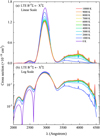 |
Fig. 7 LTE cross-sections from X2Σ+ to B′2Σ+ for temperatures between 0 K and 10 000 K. |
3.5 Photodissociation from X2Σ+ to A2Π, C2Π and E2Σ+
The photodissociation cross-sections of A2Π ←X2Σ+, E2Σ+ ← X2Σ+, and C2Π ←X2Σ+ transitions are also calculated, the complete data set is provided in the supplementary material, and the main features are discussed in this section. Figure 8 displays the cross-sections for the transitions from ν″ = 0, 4, 8, 11, and J″ = 0 of the X2Σ+ to the A2Π state. Compared with the case of B′2Σ+ ←X2Σ+ in Fig. 5, the largest peak originating from zero of a given TDM vanishes, and the cross-sections show multiple oscillating structures due to the behavior of final continuum wave functions. These features also appear in the transitions E2Σ+ ← X2Σ+ and C2Π ←X2Σ+. Figure 9 presents the cross-sections for the transitions from J″ = 0, 10, 20, 30 ,44, and ν″ = 0 of the X2Σ+ to the A2Π, E2Σ+, and C2Π states, respectively. Apparently, a number of shape resonance structures appear when the rotational quantum numbers J″ is large, as mentioned above. This is due to the large centrifugal terms and formation of a quasi-bound level. An intriguing phenomenon is observed in the ν″ = 0, J″ = 44 cross-section of the C2Π ← X2Σ+ channel, where there is a wide span of 400 Å from 2700 Å to the highest peak at 2300 Å. This distinct behavior is not commonly observed in other channels.
The LTE cross-sections at temperatures of 1000 K, 2000 K, 5000 K, and 10 000 K for the A2Π ← X2Σ+, C2Π ← X2Σ+, and E2Σ+ ← X2Σ+ transitions, respectively, are shown in Fig. 10. The cross-sections all increase with the increasing temperature, and the change becomes lesser above 5000 K. Another common feature is the existence of an oscillating structure and a number of broad and sharp peaks. In Fig. 10a, the cross-sections exhibit two broad peaks around 4240 Å and 4480 Å, both encompassing numerous oscillatory structures. This is distinct from the B′2Σ+ ← X2Σ+ LTE cross-sections, which display oscillatory structures primarily on a single broad peak. The cross-sections of the A2Π ← X2Σ+ channel is generally several orders of magnitude smaller than that of the B′2Σ+ ← X2Σ+ channel. As delineated in Tables A.3 and A.4, the band oscillator strengths of A2Π ← X2Σ+ for ν″ = ν′ surpass the B′2Σ+ ← X2Σ+ band oscillator strengths by several orders of magnitude, and the sum of Franck-Condon factors from the lowest vibrational levels to all the bound vibrational levels of A2Π state approximates to one. Conversely, the sum of Franck-Condon factors from ν″ = 0, 1, 2, and 3 of the ground state to all the bound vibrational levels of B′2Σ+, respectively, manifest as 0.85, 0.60, 0.59, and 0.60. It can be qualitatively stated that the oscillator strength from ν″=0, 1, 2, and 3 of B′ ← X contribute between 15% and 40% to the dissociation of the MgH molecule, whereas the oscillator strength of A ← X contributes a significantly smaller fraction to the dissociation process. This phenomenon was already pointed out by Kirby et al. (1979). The photodissociation cross-section of the C2Π ← X2Σ+ and E2Σ+ ← X2Σ+ channels, depicted in Figs. 10b and c, is much larger and at the same order of B′2Σ+ ← X2Σ+. The LTE cross-sections of the C2Π ← X2Σ+ channel display a wide distribution from a wavelength of 2230–2830 Å, with a broad peak occurring around 2390 Å. In contrast, the broad peak of the E2Σ+ ← X2Σ+ channel falls within the range of 2600–2810 Å.
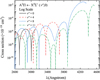 |
Fig. 8 Photodissociation cross-sections from ν″= 0, 4, 8, 11, and J″ = 0 of X2Σ+ to A2Π. |
3.6 Total LTE photodissociation cross-sections
The total LTE photodissociation cross-sections are calculated with wavelengths greater than 1800 Å, where only transitions B′2Σ+ ←X2Σ+, A2Π ←X2Σ+, C2Π ←X2Σ+, and E2Σ+ ← X2Σ+ are involved. The total and partial LTE cross-sections at 0 K are plotted in Fig. 11; these correspond to the cross-sections with a given rovibrational level (ν″ = 0, J″ = 0). Within the wavelength range of 1800–2200 Å, the C2Π ← X2Σ+ dissociation channel dominates the total cross-section at 0 K. The contribution from B′2Σ+ ← X2Σ+ and E2Σ+ ← X2Σ+ are approximately one order of magnitude lower. The thresholds of C2Π ← X2Σ+ and E2Σ+ ← X2Σ+ transitions occur at about 2200 Å wavelength. In the wavelength region above 2200 Å, the total cross-section is almost completely the same as the cross-section of B′2Σ+ ← X2Σ+. Throughout the entire range, the A2Π ← X2Σ+ channel has minimal contribution to the total cross-section, with its values predominantly below 10−9 Å2.
Simultaneously, we present the total cross-sections at different temperatures in Fig. 12. Notably, in the majority of the wavelength range (1800–840 Å and 3100–550 Å), the total cross-section generally increases with rising temperature. However, within the 2840–3100 Å range, the trend is reversed. This is exactly the behavior of the B′2Σ+ ← X2Σ+ cross-section, which plays a dominant role in this region. Except in the case of 0 K, significant oscillatory structures are observed in the total cross-sections between 2270 Å and 2840 Å, and there are minor oscillatory structures in the total cross-sections beyond 3300 Å, with a prominent peak at 4260 Å. These variations and structural features are attributed to the contributions of different dissociation channels. In the wavelength range of 1800–2840 Å, the C2Π ← X2Σ+ channel predominantly contributes to the total cross-section, with the C2Π ← X2Σ+ and E2Σ+ ← X2Σ+ channel providing some resonant peaks within the 2700 Å to 2840 Å range. Conversely, within the range of 2800 Å to 4550 Å, the total cross-sections are primarily influenced by the B′2Σ+ ← X2Σ+ channel. The resonant peak observed at 4260 Å aligns precisely with the LTE cross-section of the B′2Σ+ ← X2Σ+ channel. Additionally, some oscillatory structures around 4440 Å originate from the A2Π ← X2Σ+, although its overall contribution to the total cross-section is minimal.
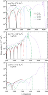 |
Fig. 9 Photodissociation cross-sections from ν″ = 0 and J″ = 0, 10, 20, 30, 44 of X2Σ+ to (a) A2Π, (b) C2Π, and (c) E2Σ+. |
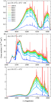 |
Fig. 10 LTE cross-sections for (a) A2Π ←X2Σ+, (b) C2Π ←X2Σ+, and (c) E2Σ+ ←X2Σ+ for temperatures between 1000 K and 10 000 K. |
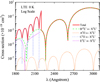 |
Fig. 11 LTE cross-sections at temperature of 0 K. |
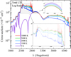 |
Fig. 12 Total LTE cross-sections for temperatures of 0 K, 1000 K, 2000 K, 5000 K, and 10 000 K. |
4 Conclusions
In this study, we employed detailed ab initio calculations to determine the PECs and TDMs of MgH, further deriving the band oscillator strength and rovibrationally resolved photodissocia-tion cross-sections. Initially, we computed the PECs for electronic states up to the atomic configurations of Mg(3s3d 1Dg)+ H(1s 2Sg) without considering the core-valence correlation. To optimize accuracy for critical low-lying states, we employed the CV-MRCI method. This integrated the core-valence correlation with 2p6 electrons of Mg and applied a complete basis set procedure, resulting in spectroscopic constants closely consistent with experimental data, with minor deviations in Re and Te of only 0.1%. Building on these precise PECs and TDMs, we detailed the photodissociation cross-sections from the 315 rovibrational levels of X2Σ+ and LTE cross-sections up to 10 000 K for wavelengths beyond 1800 Å. While our results for transitions B′2Σ+ ← X2Σ+ and A2Π ← X2Σ+ showed similarities to those of Weck et al. (2003b,a), subtle differences emerged due to our enhanced computation. Notably, this work provides the first insights into photodissociation for transitions C2Π ← X2Σ+ and E2Σ+ ← X2Σ+. Their contributions to the overall cross-section are comparable to that of B′2Σ+ ← X2Σ+. Observations in the LTE cross-sections presented characteristic oscillatory patterns and distinct resonances. Contrary to findings by Weck et al. (2003b), where an increase in the total cross-section accompanied a temperature increase, our findings showed an inverse relationship from 2840 to 3100 Å.
In summary, our detailed study of MgH’s electronic structure matches closely with recent theoretical calculations and shows strong agreement with experimental spectroscopic constants. From this, we offer precise values for the oscillator strength and photodissociation cross-sections. These insights could prove valuable to our understanding of interstellar and circumstellar chemistry, particularly in assessing MgH abundances and its chemical evolution in clouds, envelopes, and disks.
Acknowledgements
We gratefully acknowledge the support from the National Natural Science Foundation of China (Nos. 11934004, 11974230 and 12304279).
Appendix A Spectroscopic constants, band oscillator strengths and transition energies of 24MgH
Spectroscopic constants of 2Σ+ and 2Δ.
Spectroscopic constants of 2Π.
Band oscillator strengths and transition energies (cm–1) of B′2Σ+ ← X2Σ+ and A2Π ← X2Σ+, with J′ = and J″ = 0.
Band oscillator strengths and transition energies (cm–1) of C2Π ← X2Σ+ and E2Π ← X2Σ+, with J′ = 1 and J″ = 0.
Potential energy curves of X2Σ+, B′2Σ+, E2Σ+, A2Π, and C2Π in eV.
Transition dipole moments of B′2Σ+ -X2Σ+, E2Σ+-X2Σ+, A2Π-X2Σ+, and C2Π-X2Σ+ in a.u.
References
- Argyros, J. 1974, J. Phys. B: At. Mol. Phys., 7, 2025 [NASA ADS] [CrossRef] [Google Scholar]
- Barbuy, B. 1987, A&A, 172, 251 [NASA ADS] [Google Scholar]
- Bell, R. A., Edvardsson, B., & Gustafsson, B. 1985, MNRAS, 212, 497 [NASA ADS] [CrossRef] [Google Scholar]
- Bernath, P. F. 2020, Spectra of Atoms and Molecules (Oxford University Press) [Google Scholar]
- Bhattacharyya, S., & Basu, D. 1983, Chem. Phys., 79, 129 [CrossRef] [Google Scholar]
- Boutalib, A., Daudey, J., & El Mouhtadi, M. 1992, Chem. Phys., 167, 111 [CrossRef] [Google Scholar]
- Chattopadhyaya, S. 2016, Mol. Phys., 114, 3026 [NASA ADS] [CrossRef] [Google Scholar]
- Datta, K. K., Basu, D., Saha, S., & Barua, A. K. 1983, J. Phys. B: At. Mol. Phys., 16, 2377 [NASA ADS] [CrossRef] [Google Scholar]
- Dunning, T. H., Jr. 1989, J. Chem. Phys., 90, 1007 [NASA ADS] [CrossRef] [Google Scholar]
- El-Kork, N., Al Razzouk, H., Atwani, S., et al. 2018, J. Phys. Commun., 2, 055030 [CrossRef] [Google Scholar]
- Guitou, M., Spielfiedel, A., & Feautrier, N. 2010, Chem. Phys. Lett., 488, 145 [CrossRef] [Google Scholar]
- Huber, K. P., & Herzberg, G. 1979, Constants of Diatomic Molecules (Boston, MA: Springer US), 8 [Google Scholar]
- Kerkines, I. S., & Mavridis, A. 2007, J. Phys. Chem. A, 111, 371 [CrossRef] [Google Scholar]
- Kirby, K., Saxon, R., & Liu, B. 1979, ApJ, 231, 637 [NASA ADS] [CrossRef] [Google Scholar]
- Kirby, K., Van Dishoeck, E., Bates, D., & Bederson, B. 1989, Advances in Atomic Molecular Physics (New York: Academic Press) [Google Scholar]
- Knowles, P. J., & Werner, H.-J. 1985, Chem. Phys. Lett., 115, 259 [CrossRef] [Google Scholar]
- Knowles, P. J., & Werner, H.-J. 1988, Chem. Phys. Lett., 145, 514 [NASA ADS] [CrossRef] [Google Scholar]
- Knowles, P. J., & Werner, H.-J. 1992, Theor. Chim. acta, 84, 95 [CrossRef] [Google Scholar]
- Kramida, A., Yu. Ralchenko, Reader, J., & and NIST ASD Team 2022, NIST Atomic Spectra Database (ver. 5.10), available: https://physics.nist.gov/asd (National Institute of Standards and Technology, Gaithersburg, MD) [Google Scholar]
- Krebs, S., & Buenker, R. J. 1995, J. Chem. Phys., 103, 5613 [NASA ADS] [CrossRef] [Google Scholar]
- Lambert, D., Mallia, E., & Petford, A. 1971, MNRAS, 154, 265 [NASA ADS] [CrossRef] [Google Scholar]
- Langhoff, S. R., & Davidson, E. R. 1974, Int. J. Quant. Chem., 8, 61 [CrossRef] [Google Scholar]
- Leininger, T., & Jeung, G.-H. 1995, J. Chem. Phys., 103, 3942 [NASA ADS] [CrossRef] [Google Scholar]
- Lindh, R., Ryu, U., & Liu, B. 1991, J. Chem. Phys., 95, 5889 [NASA ADS] [CrossRef] [Google Scholar]
- London, F. 1937, Trans. Faraday Soc., 33, 8b [CrossRef] [Google Scholar]
- McWilliam, A., & Lambert, D. L. 1988, MNRAS, 230, 573 [NASA ADS] [CrossRef] [Google Scholar]
- Mestdagh, J.-M., De Pujo, P., Soep, B., & Spiegelman, F. 2009, Chem. Phys. Lett., 471, 22 [NASA ADS] [CrossRef] [Google Scholar]
- Miyake, S., Gay, C., & Stancil, P. 2011, ApJ, 735, 21 [NASA ADS] [CrossRef] [Google Scholar]
- Mostafanejad, M., & Shayesteh, A. 2012, Chem. Phys. Lett., 551, 13 [NASA ADS] [CrossRef] [Google Scholar]
- Müller, T. 2006, Computat. Nanosc., 19 [Google Scholar]
- Murrell, J. N. 1984, Molecular Potential Energy Functions (John Wiley) [Google Scholar]
- Qin, Z., Bai, T., & Liu, L. 2021, ApJ, 917, 87 [NASA ADS] [CrossRef] [Google Scholar]
- Qin, Z., Bai, T., & Liu, L. 2022, MNRAS, 516, 550 [NASA ADS] [CrossRef] [Google Scholar]
- Saxon, R., Kirby, K., & Liu, B. 1978, J. Chem. Phys., 69, 5301 [NASA ADS] [CrossRef] [Google Scholar]
- Shayesteh, A., & Bernath, P. F. 2011, J. Chem. Phys., 135, 094308 [NASA ADS] [CrossRef] [Google Scholar]
- Shayesteh, A., Appadoo, D. R. T., Gordon, I., Le Roy, R. J., & Bernath, P. F. 2004, J. Chem. Phys., 120, 10002 [NASA ADS] [CrossRef] [Google Scholar]
- Shayesteh, A., E, H. D., Gordon, I., Le Roy, R. J., & Bernath, P. F. 2007, J. Chem. Phys. A, 111, 12495 [NASA ADS] [CrossRef] [Google Scholar]
- Skory, S., Weck, P., Stancil, P., & Kirby, K. 2003, ApJS, 148, 599 [NASA ADS] [CrossRef] [Google Scholar]
- Wang, K., Wang, X., Fan, Z., et al. 2021, Eur. Phys. J. D, 75, 1 [CrossRef] [Google Scholar]
- Watson, J. K. 2008, J. Mol. Spectrosc., 252, 5 [NASA ADS] [CrossRef] [Google Scholar]
- Weck, P., Schweitzer, A., Stancil, P., Hauschildt, P., & Kirby, K. 2003a, ApJ, 584, 459 [NASA ADS] [CrossRef] [Google Scholar]
- Weck, P., Stancil, P., & Kirby, K. 2003b, ApJ, 582, 1263 [NASA ADS] [CrossRef] [Google Scholar]
- Werner, H.-J., & Knowles, P. J. 1985, J. Chem. Phys., 82, 5053 [NASA ADS] [CrossRef] [Google Scholar]
- Werner, H.-J., & Knowles, P. J. 1988, J. Chem. Phys., 89, 5803 [NASA ADS] [CrossRef] [Google Scholar]
- Werner, H.-J., Knowles, P. J., Knizia, G., et al. 2012, MOLPRO, version 2012.1, a package of ab initio programs https://www.molpro.net/ [Google Scholar]
- Wilson, A. K., Woon, D. E., Peterson, K. A., & Dunning, T. H. 1999, J. Chem. Phys., 110, 7667 [NASA ADS] [CrossRef] [Google Scholar]
- Woon, D. E., & Dunning, T. H., Jr. 1993, J. Chem. Phys., 98, 1358 [NASA ADS] [CrossRef] [Google Scholar]
- Yang, Y. K., Cheng, Y., Peng, Y. G., et al. 2020, JQSRT, 254, 107203 [NASA ADS] [CrossRef] [Google Scholar]
- Zhu, Z. 2007, Sci. China Ser. G: Phys. Mech. Astron., 50, 581 [NASA ADS] [CrossRef] [Google Scholar]
All Tables
Band oscillator strengths and transition energies (cm–1) of B′2Σ+ ← X2Σ+ and A2Π ← X2Σ+, with J′ = and J″ = 0.
Band oscillator strengths and transition energies (cm–1) of C2Π ← X2Σ+ and E2Π ← X2Σ+, with J′ = 1 and J″ = 0.
Transition dipole moments of B′2Σ+ -X2Σ+, E2Σ+-X2Σ+, A2Π-X2Σ+, and C2Π-X2Σ+ in a.u.
All Figures
|
Fig. 1 Potential energy curves. (a) Solid lines: NCV-MRCI results. Dashed lines: CV-MRCI results. Dotted lines: Mestdagh et al. (2009). Dashed-dotted lines: El-Kork et al. (2018). Triangles: Guitou et al. (2010). (b) Solid lines: NCV-MRCI results. Dashed lines: CV-MRCI results. Dotted lines: Saxon et al. (1978). Dashed-dotted lines: Chattopadhyaya (2016). Triangles: Mostafanejad & Shayesteh (2012). |
| In the text | |
|
Fig. 2 Transition dipole moments of B′2∑+–X2∑+, A2Π–X2∑+, C2π–X2∑+ and E2∑+–X2∑+ for MgH. Solid lines: CV-MRCI calculations. Dashed lines: NCV-MRCI calculations. Dotted lines: Chattopadhyaya (2016). Solid lines with stars: El-Kork et al. (2018). Solid lines with triangles: Saxon et al. (1978). Solid lines with circles: Mostafanejad & Shayesteh (2012). |
| In the text | |
|
Fig. 3 Photodissociation cross-sections from X2∑+ to B′2∑+. (a) (v″, J″) = (0, 0) and (b) (v″, J″) = (0, 18). |
| In the text | |
|
Fig. 4 Photodissociation cross-sections from J″ = 0 and v″ = 0–11 of x2∑+ to B′2∑+. |
| In the text | |
|
Fig. 5 Photodissociation cross-sections from v″ = 0 and J″ = 0, 5, 10, 20, 35, 40, 44 of X2∑+ to B′2∑+. |
| In the text | |
|
Fig. 6 Photodissociation cross-sections from v″ = 4 and J″ = 0, 20, 28, 32 of X2∑+ to B′2∑+. |
| In the text | |
|
Fig. 7 LTE cross-sections from X2Σ+ to B′2Σ+ for temperatures between 0 K and 10 000 K. |
| In the text | |
|
Fig. 8 Photodissociation cross-sections from ν″= 0, 4, 8, 11, and J″ = 0 of X2Σ+ to A2Π. |
| In the text | |
|
Fig. 9 Photodissociation cross-sections from ν″ = 0 and J″ = 0, 10, 20, 30, 44 of X2Σ+ to (a) A2Π, (b) C2Π, and (c) E2Σ+. |
| In the text | |
|
Fig. 10 LTE cross-sections for (a) A2Π ←X2Σ+, (b) C2Π ←X2Σ+, and (c) E2Σ+ ←X2Σ+ for temperatures between 1000 K and 10 000 K. |
| In the text | |
|
Fig. 11 LTE cross-sections at temperature of 0 K. |
| In the text | |
|
Fig. 12 Total LTE cross-sections for temperatures of 0 K, 1000 K, 2000 K, 5000 K, and 10 000 K. |
| In the text | |
Current usage metrics show cumulative count of Article Views (full-text article views including HTML views, PDF and ePub downloads, according to the available data) and Abstracts Views on Vision4Press platform.
Data correspond to usage on the plateform after 2015. The current usage metrics is available 48-96 hours after online publication and is updated daily on week days.
Initial download of the metrics may take a while.