| Issue |
A&A
Volume 684, April 2024
|
|
|---|---|---|
| Article Number | A135 | |
| Number of page(s) | 11 | |
| Section | Galactic structure, stellar clusters and populations | |
| DOI | https://doi.org/10.1051/0004-6361/202348781 | |
| Published online | 16 April 2024 | |
Stellar halo density with LAMOST K and M giants
1
Instituto de Astrofísica de Canarias, 38205 La Laguna, Tenerife, Spain
e-mail: This email address is being protected from spambots. You need JavaScript enabled to view it.
2
PIFI-Visiting Scientist 2023 of Chinese Academy of Sciences at Purple Mountain Observatory, Nanjing 210023, and National Astronomical Observatories, Beijing 100012, PR China
3
Departamento de Astrofísica, Universidad de La Laguna, 38206 La Laguna, Tenerife, Spain
4
School of Physics and Astronomy, China West Normal University, 1 ShiDa Road, Nanchong 637002, PR China
5
Institute for Frontiers in Astronomy and Astrophysics, Beijing Normal University, Beijing 102206, PR China
6
Key Laboratory of Space Astronomy and Technology, National Astronomical Observatories, Chinese Academy of Sciences, Beijing 100101, PR China
7
Dipartimento di Fisica e Astronomia, Università di Padova, Vicolo dell’Osservatorio 3, 35122 Padova, Italy
8
University of Chinese Academy of Sciences, Beijing 100049, PR China
Received:
29
November
2023
Accepted:
5
February
2024
Abstract
Aims. We derive the morphology of the stellar component in the outer halo volume, and search for possible overdensities due to substructures therein.
Methods. We made use of some of the data releases of the spectroscopic survey LAMOST DR8-DR9 in tandem with distance determinations for two subsamples, that is, of K-giants and M-giants, respectively, making up 60 000 stars. These distance are obtained through Bayesian techniques that derive absolute magnitudes as a function of measured spectroscopic parameters. Our calculation of the density from these catalogues requires: (1) derivation of the selection function; and (2) a correction for the convolution of the distance errors, which we carried out with Lucy’s inversion of the corresponding integral equation.
Results. The stellar density distribution of the outer halo (distance to the Galactic centre, rG, of between 25 and 90 kpc) is a smooth monotonously decreasing function with a dependence of approximately ρ ∝ rG−n, with n = 4.6 ± 0.4 for K-giants and n = 4.5 ± 0.2 for M-giants, and with a insignificant oblateness. The value of n is independent of the angular distance to the Sagittarius tidal stream plane, which is what would be expected if such a stream did not exist in the anticenter positions or had a negligible imprint in the density distribution in the outer halo. Apart from random fluctuations or minor anomalies in some lines of sight, we do not see substructures superimposed in the outer halo volume within the resolution that we are using and limited by the error bars. This constrains the mass of over- and under-densities in the outer halo to be of ≲103 M⊙ deg−2, whereas the total mass of the stellar halo, including inner and outer parts, is ∼7 × 10⁸ M⊙.
Key words: Galaxy: halo / Galaxy: structure
© The Authors 2024
 Open Access article, published by EDP Sciences, under the terms of the Creative Commons Attribution License (https://creativecommons.org/licenses/by/4.0), which permits unrestricted use, distribution, and reproduction in any medium, provided the original work is properly cited.
This article is published in open access under the Subscribe to Open model. This email address is being protected from spambots. You need JavaScript enabled to view it. to support open access publication.
1. Introduction
The stellar halo density distribution has been analysed many times (e.g., Young 1976; Fenkart 1989; Juric et al. 2008; Bilir et al. 2008; Deason et al. 2014; Xue et al. 2015, 2018; Hernitschek et al. 2018; Thomas et al. 2018; Fukushima et al. 2019; Wu et al. 2022). The representation of this component is usually given by a smooth density function monotonously decreasing for increasing Galactocentric distances, and with some possible oblateness.
Furthermore, some recent studies have pointed out the superposition of some substructures (Helmi 2020), large overdensities on the sky, and many narrow streams (Bernard et al. 2016; Shipp et al. 2018; Han et al. 2022; Wu et al. 2022) tentatively associated with the tidal streams of corresponding passages of satellites. These discoveries were motivated by prior cosmological hypotheses within the ΛCDM model, in which halos are mostly formed by accretion and merger events, encouraging astronomers to find structures similar to those predicted by simulations. However, there is no information on the distance of most of these overdensities and it is not yet clear whether these substructures correspond to a small or negligible number of stars as fluctuations embedded in the main field of the halo or to a major part of the stellar component at large Galactocentric distances.
An accurate distance determination is essential for studying the morphology in the outer Galaxy, which is not reachable with Gaia parallaxes; in any case, Gaia distances estimated with the Bailer-Jones et al. (2021) method are not useful for Galactic structure analyses because this method is dependent on assumptions for the density distribution of the Galaxy. An interesting possibility is to employ variable stars such as RR-Lyrae as standard candles (e.g., Hernitschek et al. 2018). Distance determinations from colour and photometric metallicities (e.g., Huang et al. 2023) are moderately reliable, but are not as accurate as spectroscopic distances. The available spectroscopic surveys and the most recent calibrations of the distance of far away sources therefore allow us to better constrain the morphology of the outer halo.
To this end, in this study we present an analysis that makes use of some of the latest data releases of the LAMOST survey (Yan et al. 2022), and distance determinations of two subsamples, namely of K-giants and M-giants. We apply Bayesian techniques in an analysis of these data to derive absolute magnitudes as a function of measured spectral parameters. Details of the data used in this paper are given in Sect. 2.
Calculation of the density from a given catalogue is not straightforward. There are two major technical problems to overcome in this pursuit, which are (1) the calculation of the ratio of the number of stars in our catalogue with respect to the total number of a given type, for which we hope to derive the selection function (see Sect. 3); and (2) the correction for the convolution of the distance errors (see Sect. 4).
We present the application of our method to LAMOST K and M giants in Sects. 5 and 6. In Sect. 7, we compare the results with theoretical models of the halo to derive the power law that best fits the data of the outer halo. In Sect. 8, we provide a discussion and conclusions.
2. Data
The LAMOST survey (Yan et al. 2022) covers the almost complete sky area with declination of between −10 and +60 deg. Here, we use subsamples derived from data releases 8 and 9, respectively, which collectively account for around 60 000 stars.
2.1. M-giants
A sample of LAMOST-DR9 M-giants is taken from Qiu et al. (2023), who use the Bayesian method developed by Zhang et al. (2020) to obtain the distance of more than 43 000 stars from the measured spectral parameters. After removing stars with the parameters |KabsD − KabsM|> 0.01 (where KabsD and KabsM are the K band absolute magnitude derived from the distance and the model respectively; see Qiu et al. 2023), we are left with 40 973 stars. Figure 1 shows the distribution of these stars in the sky.
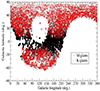 |
Fig. 1. Sky distribution of LAMOST sources used in this paper: M-giants are colour-coded in black, K-giants in red. |
Although referred to as M-giants, the range of spectral types in reality includes giants (−0.4 < log g < 2.5) between K3 and M3 spectral type, according to the selected temperatures (3200 K < Teff < 4300 K). The relative abundance of these spectral types is similar in the halo and the disc (Wainscoat et al. 1992), and therefore, in principle, we expect that most of these stars at large Galactocentric distance are genuine halo stars. The range of metallicities of these stars is −1.5 < [M/H]< 0.5, a range not introduced by us but characteristic of the training samples of the SLAM (Stellar LAbel Machine) algorithm used to generate the catalogue of Qiu et al. (2023) from LAMOST. Within this constraint on metallicity, approximately half of the halo stars get removed (López-Corredoira et al. 2018). Still, half of the halo stars remain, together with disc stars and possible tidal streams. This is taken into account in the comparison with models presented below.
2.2. K-giants
The sample of LAMOST-DR8 K-giants is taken from Zhang et al. (2023), who use the Bayesian method developed by Xue et al. (2014; and applied to SDSS-SEGUE) to obtain the distance of 19 521 stars from the measured spectroscopic parameters. Figure 1 shows the distribution of these stars in the sky, which is the same as for the M-giants, because they are derived from the same LAMOST survey, but avoiding the Galactic plane.
Although indicated as K-giants, the range of spectral types includes giants between G1 and K4, according to the selected temperatures (4000 < Teff < 5600 K). The selection criteria are: |z|> 5.0 kpc; [Fe/H] < −1.0 if 2.0 kpc < |z|< 5.0 kpc; and the error in distance is lower than 30%. This set of criteria filter out almost all of the stars of the disc, and yield an almost complete sampling of the halo stars for |z|> 2 kpc (once corrected for the selection function). We assume that the number of halo stars with [Fe/H] ≥ −1.0 is negligible. The maximum heliocentric distance is over 120 kpc, which we take here as a limit.
3. Selection function correction
The selection function for each line of sight of Galactic coordinates ℓ, b and heliocentric distance r is defined as
 (1)
(1)
The first two factors (Chen et al. 2018; Wang et al. 2018) account for the ratio of stars with measured parameters among LAMOST sources, and the number of stars with LAMOST spectroscopy (Nspec.(r)) observed at position r with respect to the total photometric sources at 2MASS Nphot.(r), respectively.
For the calculation of the first two factors, we employ the Bayesian method as mentioned by Liu et al. (2017). We obtain the position information (right ascension (RA) and declination (Dec)) for each plate from LAMOST and use Astroquery to retrieve 2MASS photometric data within a 20 deg2 region centred on that location. By combining the distribution of photometry and spectroscopy in colour–magnitude diagrams (CMDs), we derive  , including the dependence on colour c and magnitude m. All CMD bins have a size of Δc = Δ(J − K) = 0.1 dex and ΔK = 0.25 dex, and each CMD contains 2806 2D colour–magnitude bins. Finally, we stored the selection functions for 5533 plates of LAMOST DR9, with each plate having 2806 selection coefficients, and did the same with the plates of LAMOST DR8.
The third factor in Eq. (1) is an estimation of the completeness of the photometric survey 2MASS with respect to the real distribution due to the upper magnitude limit; we calculate it as:
![Mathematical equation: $$ \begin{aligned}&\left\langle \frac{N_{\rm phot.}(\boldsymbol{r})}{N_{\rm total}(\boldsymbol{r})}\right\rangle _{r; \ell , b} =\frac{\int _{-\infty }^{M_{K,\mathrm{lim}}(r;\ell , b)}\mathrm{d}M^{\prime }\,\phi (M^{\prime })}{\int _{-\infty }^{\infty }\mathrm{d}M^{\prime }\,\phi (M^{\prime })} , &M_{K,\mathrm{lim}}(r;\ell ,b)=m_{K,\mathrm{lim.}}-5\log _{10}[r(\mathrm{pc})]+5-A_K(r;\ell ,b) ,\nonumber \end{aligned} $$](/articles/aa/full_html/2024/04/aa48781-23/aa48781-23-eq4.gif) (2)
(2)
where mK, lim. = 14.3 is the K limiting magnitude of the 2MASS survey (with completeness 100% and 10σ detection), AK is the extinction in K-band (Green et al. 2019), and ϕ(M) is the luminosity function of our stars (see Fig. 2). We note that we use the parameters of the 2MASS survey in the evaluation of this third factor instead of the LAMOST survey, because the first two factors of completeness were calculated with respect to the 2MASS survey; however, we detect sources in LAMOST that are fainter than mK, lim. = 14.3. We derive the luminosity function from our sample within 2 kpc < r < 5 kpc for M-giants, and within 15 kpc < r < 20 kpc for K-giants and assume that we can extrapolate these to longer distances. In these ranges of heliocentric distances, our sample covers the whole range of absolute magnitudes: we illustrate this in Fig. 3 for K-giants, where we can see that, for r < 15 kpc, there is a lack of the brightest stars in our sample, which we tentatively believe to be due to saturation, and for r > 20 kpc we cannot see the faintest stars because these are beyond the completeness limit of LAMOST (not the same as the 2MASS 100% completeness limit). However, we note that, even in this range, we are not 100% complete in 2MASS, and this subsample may be complete to approximately > 90%; in any case, we neglect here this ≲10% correction in the third factor. However, we take into account the first two factors of the selection function.
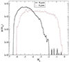 |
Fig. 2. Luminosity function of our two samples. |
Xue et al. (2015, Fig. 4), based on SDSS-SEGUE data, found that the limiting magnitude of K-giants is dependent on metallicity. In Fig. 3, we show the dependence of absolute magnitude on metallicity within the covered ranges in our LAMOST sample, and we do not find a remarkable dependence, except for [Fe/H] > −1, which might be part of some disc contamination. We therefore do not consider any dependence on metallicity in our analysis.
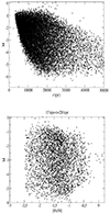 |
Fig. 3. Absolute magnitude of the K-giant sources as a function of their heliocentric distance, and as a function of [Fe/H] for the subsample with r between 15 and 20 kpc. |
In the solar neighbourhood, the value of S varies from 0.7 to 8 × 10⁻³ in the most distant regions with r ∼ 80 kpc for the M giants sample, and between 0.5 and 2 × 10⁻⁴ for the K giants sample (up to a heliocentric distance of 120 kpc).
We calculate the average density of sources within each line of sight with solid angle ω as a function of heliocentric distance r:
 (3)
(3)
where Nparam.(r)dr is the observed number of stars with spectra and measured parameters with a heliocentric distance of between r − dr/2 and r + dr/2. This ρ0 stems from a direct estimation of the density, but it is not yet corrected for the effects of the convolution of errors.
4. Lucy’s method on the deconvolution of the distance error
Due to the errors in the distances of stars, with rms σ(r), the observed density ρ0 corresponding to the distribution of stars along a given line of sight is related to the real density ρ through:
 (4)
(4)
where
![Mathematical equation: $$ \begin{aligned} K(r,t)=A(r)\,t^2\,\exp \left[-\frac{(t-r)^2}{2\sigma (r)^2}\right] ,\end{aligned} $$](/articles/aa/full_html/2024/04/aa48781-23/aa48781-23-eq7.gif) (5)
(5)
which corresponds to a Gaussian distribution of errors. A(r) stands for the normalisation such that  for all r.
Here, we assume that the error on the distance is 21% for the M-giants sample, as derived by Qiu et al. (2023); that is, σ(r) = 0.21 r. For the K-giants sample, a power-law fit of the error of the distance as a function of the distance yields an average σ(r) = 0.16 r(kpc)0.94 kpc.
The error distribution is of the kind of Fredhold integral equation of the first type with kernel K, and can be inverted with some iterative method, such as ‘Lucy’s method’ (López-Corredoira & Sylos Labini 2019):
![Mathematical equation: $$ \begin{aligned} \rho ^{[n+1]}(r)&=\rho ^{[n]}(r)\frac{\int _0^\infty \frac{\rho _{0}}{\rho _{L,[n]}(s)}K(r,t)\mathrm{d}t}{\int _0^\infty K(r,t)\mathrm{d}t} ,\end{aligned} $$](/articles/aa/full_html/2024/04/aa48781-23/aa48781-23-eq9.gif) (6)
(6)
![Mathematical equation: $$ \begin{aligned} \rho _{L,[n]}(s)&=\int _0^\infty \rho ^{[n]}(t)K(s,t)\mathrm{d}t . \end{aligned} $$](/articles/aa/full_html/2024/04/aa48781-23/aa48781-23-eq10.gif) (7)
(7)
With a few iterations (determined with the algorithm of López-Corredoira & Sylos Labini (2019); when ρL, [n](s)) ≈ ρ0(r) within the error bars, and with a minimum of 3 iterations and a maximum of 15), we get the inversion of the integral equation: ρ(r)≈ρ[n](r). The initial iteration may be set as ρ[0](r) = ρ0(r), but the result of the inversion is independent of the initial iteration assumption. Also, we note that this method is model independent, as it does not assume any priors about the shape of the density. The results of this inversion method have been compared to those from Monte Carlo simulations in previous papers presenting applications to the deconvolution of Gaia parallaxes (López-Corredoira & Sylos Labini 2019; Chrobáková et al. 2020).
5. Example application to entire samples
Let us consider the average of the whole sky coverage of both samples: for M-giants, ω = 6.6 stereo-radians, assuming that all the sources with declination between −10 and +60 deg are observed; for K-giants, we add the extra constraint of avoiding regions within |z|< 2 kpc, which gives a ω of between 4.3 and 6.5 stereo-radians, depending on the distance. We calculate the average density of observed sources as a function of heliocentric distance r. The result is plotted in log–log (step: Δlog10(r) = 0.04) in Fig. 4 as a function of heliocentric distance and Fig. 5 as a function of the distance to the Galactic centre,  .
.
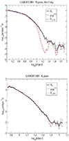 |
Fig. 4. Stellar density as a function of heliocentric distance for M-giants (top panel; 40 973 sources) and K-giants (bottom panel; 19 521 sources). ρ0 is the observed density without correction of deconvolution or parallax errors; ρ is the density with deconvolution; ρL, [15] is the amount derived in Eq. (7), which converges to ρ0 after 15 iterations. |
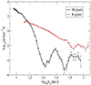 |
Fig. 5. Stellar density after deconvolution correction as a function of the distance to Galactic centre for M-giants (top panel; 40 973 sources) and K-giants (bottom panel; 19 521 sources). Error bars correspond to the Poissonian errors of the measured ρ0. |
In the profile ρ0(r) for M-giants, we observe two ranges, that is, closer than and beyond 20 kpc (log10r(kpc) = 1.3), which might be interpreted as the volumes where the disc and halo are predominant, respectively. It is also observed that the density is monotonously decreasing. Nonetheless, this observed density is not correct; rather it corresponds to the convolution of the real density, as expressed in Eq. (4). When we apply the previous method of deconvolution to this ρ0(r), we obtain ρ(r) as shown in the red-dashed line in the upper panel of Fig. 4. As expected, the density ρ(r) in the outer region (r > 10 kpc) is much lower than ρ0(r). Remarkably, one can see that the real density is not monotonously decreasing, but there are two minima of the density around r = 18 kpc (log10r(kpc) = 1.25) and r = 45 kpc (log10r(kpc) = 1.65), and then two substructures appear with peaks around r = 28 and r = 63 kpc (log10r(kpc) = 1.45, log10r(kpc) = 1.80). This shows the power of this method in recovering information on the density, and highlights some structures that were masked by the convolution of errors. However, these types of under-densities and over-densities only represent an average within areas in the first three quadrants; the combination of areas with different depth might produce this kind of artefact. In order to check for the possible existence of substructures, in the following section we examine the analysis with more accurate space resolution, separating different lines of sight only in the second and third quadrant, which allows us to distinguish structures not only as a function of distance but also of the position in the sky.
For the K-giants, the effect of Lucy’s deconvolution is less significant, because the error on the distance σ(r) is much smaller than for M-giants. This survey has removed the Galactic plane and has a predominant contribution to the density at high latitudes. Again, there can be no direct interpretation of the under-densities and peaks in ρ(r) because we are combining many different lines of sight and we need to separate these to derive the mean density along them. Nonetheless, the exercise in this section serves to illustrate the application of the methodology.
6. Different lines of sight
We apply this method of deconvolution (together with the selection function analysis) to different lines of sight corresponding to different subsamples of LAMOST to derive the star density. The different results of the deconvolution are shown in Fig. 6.
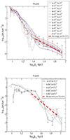 |
Fig. 6. Stellar density after deconvolution correction as a function of the distance to the Galactic centre. Upper panel: M-giants within 12 lines of sight with Δb = 5°, Δℓ = 10°. Bottom panel: K-giants within five lines of sight with Δb = 15°, Δℓ = 30 ° /cos(b). Fits correspond to the average of all lines of sight in the range log10[rG(kpc)] between 1.4 and 1.95, except the line ℓ = 154°, b = −52.5°, which presents an anomaly. Error bars (corresponding to the error of measured ρ0) of the first line of sight are plotted; for other lines of sight, the error bars are similar. |
For the M-giants sample, we divide the sky within 90 ° < ℓ< 270° in regions with Δb = 5°, Δℓ = 10°; the area of these regions is 50 square degrees when they are totally covered by the LAMOST survey or lower otherwise. We consider only the areas with more than 400 stars. This results in a total of 12 regions, all of them within |b|≤10°, and with a covered area of larger than 47.9 deg2 each. We run the Lucy’s deconvolution method on them using a step of Δlog10(r) = 0.1.
They show a monotonously decreasing density, typical of a halo density distribution, with no significant dependence on the latitude. This indicates a low oblateness of the halo; the exception is the line of sight toward ℓ = 155°, b = −2.5°, which presents a relative peak at rG ≈ 23 kpc.
For the K-giants sample, we have a lower number of stars per square degree, and so we take larger areas: we divide the sky within 90 ° < ℓ< 270° in regions with Δb = 15°, Δℓ = 30 ° /cos(b). We only consider the areas with more than 400 stars: a total of five regions, all of them off-plane, with a covered area of each line of sight of between 170 and 360 deg2. We run the Lucy’s deconvolution method on them using a step of Δlog10(r) = 0.1. In general, the density of these areas shows a similar dependence on the distance to that of the centre of the Galaxy: a monotonously decreasing density typical of a halo density distribution, with no significant dependence on the latitude, which again indicates a low oblateness of the halo; the exception is the line of sight toward ℓ = 154°, b = −52.5°, which exhibits a relative peak at rG ≈ 25 kpc.
For K-giants, the five selected lines of sight are clearly separated and do not allow us to build a 3D map. For the M-giant lines of sight, which are more continuous and confined in the plane, we combine the derived densities of the 12 of them to produce a 3D map in Galactocentric coordinates (we assume R⊙ = 8 kpc and we neglect the height of the Sun over the plane: Z⊙ = 0). In Fig. A.1, we plot three slices of this 3D map parallel to the XY plane, corresponding to −6 kpc < Z < −2 kpc, |Z|< 2 kpc, and 2 kpc < Z < 6 kpc, respectively. In Fig. A.2 we plot the density ρ0 (without deconvolution) only for the plane region for comparison; and in Fig. A.3 we show the corresponding counts of stars per unit volume.
These maps indicate a smooth distribution without clear substructures above the noise level. There are no significant over-densities and the only remarkable under-density is for Y = −20 to −10, X = 40 to 80, Z = −6 to 0 (units are in kpc), which corresponds to just one line of sight ℓ = 195°, b = −2.5°. Figure 6 shows how the density along this line of sight for all distances is much lower than the density in the other lines of sight, but with the same monotonously decreasing power-law shape. Given that there are no signs of structure with peaks or valleys along this line of sight, we attribute the global under-density for this line of sight to some possible loss of stars or miscalibration of extinction or the selection function in LAMOST.
The maps of Fig. A.1 show that the density of stars after applying Lucy’s deconvolution at the largest R is much lower than that without this correction: from Fig. 6 (M-giants at R > 40 kpc), this density is ≲2.5 × 10⁻³ kpc−3 (≲10−6 times the solar neighbourhood density); at R > 70 kpc, it is ≲5 × 10⁻⁴ kpc−3 (≲2 × 10⁻⁷ times the solar neighbourhood density). Two orders of magnitude larger densities are found for K-giants in off-plane regions for similar Galactocentric distances ( ), which we attribute to the larger number of K-giants than M-giants.
The observed density of M-giants in the solar neighbourhood in Fig. 6 is ρ⊙, M-giants ∼ 2.5 × 10³ star kpc−3 (this is dominated by disc stars). For K-giants, we have no direct density measurements in the solar neighbourhood (the Galactic plane stars were removed), but we estimate a ratio of K-giants/M-giants of ∼101.6 (derived as the average from Fig. 6 in the range of log rG = 1.4 − 1.9, where the disc does not contribute and neglecting the oblateness of the halo), and so this would imply ρ⊙, K-giants ∼ 105 star kpc−3.
7. Halo density
Most of the regions with R > 25 kpc or |z|> 4 kpc should be explained in terms of halo density. For comparison, Fig. A.4 shows the prediction of the density of stars in the halo following the model by Fenkart (1989) and Bilir et al. (2008):
![Mathematical equation: $$ \begin{aligned} \rho _{\rm halo}&=1.4\times 10^{-3}f\,\rho _\odot \frac{\exp [Q (1-X_{\rm sp}^{0.25})]}{X_{\rm sp}^{0.875}}, & X_{\rm sp}&=\frac{\sqrt{X^2+Y^2+(Z/q)^2}}{R_\odot }\nonumber \end{aligned} $$](/articles/aa/full_html/2024/04/aa48781-23/aa48781-23-eq14.gif) (8)
(8)
where Q = 10.093 and q = 0.63. In the case of M-giants, we add an extra factor f = 0.5 in the normalisation to take into account the fact that in the observed range of metallicities we include all the M-giants of the disc but only ∼50% of the M-giants in the halo (López-Corredoira et al. 2018); for the K-giants sample, we take f = 1.
For M-giants, comparing Fig. A.4 with the central panel of Fig. A.1, we see that Fenkart (1989) and Bilir et al. (2008) predict a similar density to that observed at large Galactocentric distances. We can therefore say that most of the stars at X > 25 kpc can be explained in terms of the stellar halo and there is no need for extragalactic components or multiple substructures. Of course, at X < 25, the halo model gives much lower stellar density than observed because the disc dominates in that volume.
Another model derived by Xu et al. (2018) provides a parametrisation of
 (9)
(9)
where n = 5.03 and q ≈ 1 for Xsp > 4. With this new profile, and adopting the same normalisation as above, AX, ⊙ = 1.4 × 10⁻³f ρ⊙, we get the density distribution plotted in Fig. A.5. This second model yields much lower densities of M-giants than our data in the outer parts. Instead, with this simple law of Eq. (9), we would need n = 4.52 ± 0.21 with M-giants and n = 4.61 ± 0.36 with K-giants (see fits of Fig. 6 in the range log10[rG(kpc)] between 1.40 and 1.95). This value of n is very similar to the one obtained in other previous analyses (e.g., Xue et al. 2015; Hernitschek et al. 2018), although, as opposed to these latter authors, we do not find clear fluctuations or variations indicative of possible substructures. In Table 1, we give the values of n for each line of sight, and in Fig. A.6, we show the residuals with respect to these fits in that range of rG. In the case of M-giants, these are within Poissonian errors; in the K-giants, fluctuations are larger than Poissonian errors but still small and random, without any clear defined structure. In Fig. A.7, we show a plot that is similar to the bottom panel of Fig. 13 of Hernitschek et al. (2018), with variation of the average slope n with the sky position in the 17 investigated lines of sight. This variation of n appears to be random and not associated to particular regions of the sky. In general, apart from the anomalies already pointed out in the previous section, no significant coherent variations of the slope or fluctuations are observed.
Best linear fits of the density profile in log–log, log10(ρ) = A − n(x − 1.40), x = log10[rG(kpc)], in the range log10[rG(kpc)] between 1.40 and 1.95 for the different lines of sight.
Of these 17 lines of sight, 7 have their centre at an angular distance of lower than 10 degrees from the main Sagittarius stream orbit, which might affect the determination of the slope of the smooth halo profile (Thomas et al. 2018). If we calculate the power-law index n only with the lines of sight with  deg, we get n = 4.50 ± 0.18 for M-giants and n = 4.57 ± 0.56 for K-giants. No significant difference with respect to the values of n including the lines of sight close to Sagittarius stream orbit. In Fig. A.8, we plot n versus
  . We do not find any correlation. Sagittarius stream regions provide a negligible contribution to the change of the halo profile. We could even conclude that our data are compatible with no detection at all of such a putative tidal stream.
By performing the inverse calculation of star counts with this power-law distribution, using Eq. (3), the number of observed (with spectra) stars with Galactocentric distance (rG) larger than rG, min should be
 (10)
(10)
Assuming a selection function  , ωG, the angular area of the sky observed from a Galactocentric position (which is not the same thing as ω, which is the area observed in heliocentric coordinates, but they are similar at large R, and so we can assume ωG = ω = 6.5 stereo-radians) is equal to
 (11)
(11)
where n = 4.6 for both samples. For our samples, we measure: AX, ⊙ = 1.7 kpc−3, S(50 kpc) = 0.5, β = 7.6 for M-giants; AX, ⊙ = 140 kpc−3, S(50 kpc) = 0.07, β = 4.0 for K-giants. With these parameters, the number of halo stars with rG larger than 50 kpc would be ∼16 M-giants and ∼310 K-giants. These numbers are close to the observed number of stars with rG > 50 kpc: 10 M-giants; 273 K-giants (Zhang et al. 2023).
The total number of stars of the halo for rG, min > 4 kpc (neglecting the oblateness terms and including those that are not M-giants or K-giants, within MG < 10) can also be derived from Eq. (11) by setting rG, min = 4 kpc, S(4 kpc) = 1, β = 0, ω = 4π, AX, ⊙ = 1.4 × 10⁻³ρ⊙ and assuming a total stellar density (including disc and halo) within MG < 10 of ρ⊙ = 6.4 × 10⁷ kpc−3 (Chrobáková et al. 2020). This results N ∼ 109 stars. The stellar mass density of solar neighbourhood is 4.3 × 10⁷ M⊙ kpc−3 (McKee et al. 2015), and therefore the ratio of mass per star (for stars with MG < 10) in the solar neighbourhood is 2/3 M⊙/star.hi This ratio is subject to some uncertainties, but the order of magnitude is not expected to change significantly. Assuming a similar mass per star ratio in the disc and in the halo, we would have a total mass of the stellar halo at R > 4 kpc of ∼7 × 10⁸ M⊙. This number is similar to other values estimated in the literature, which give 4 − 7 × 10⁸ M⊙ (review at Bland-Hawthorn & Gerhard 2016).
The stellar mass estimated with the same procedure for the outer halo (rG > 25 kpc) gives ∼4 × 10⁷ M⊙. The fluctuations of the density in the top panel of Fig. 6 are Δlog10ρ ∼ 0.6 within 50 square degrees (1/800 of sky area), which means that possible substructures in the outer halo within the level of the fluctuations should have a mass of ≲6 × 10⁴ M⊙, that is, ≲103 M⊙ deg−2.
8. Discussion and conclusions
The outer halo stellar density distribution is a smooth monotonously decreasing function of the distance to the Galactic centre, rG, with a dependence of approximately  , with n ≈ 4.6 for K-giants and n ≈ 4.5 for M-giants, which are compatible with each another.
We did not investigate the halo oblateness (Juric et al. 2008) or prolateness (Thomas et al. 2018; Fukushima et al. 2019) found by other authors. The halo should be almost spherical at the large Galactocentric distances explored in the present study (Xu et al. 2018), and indeed we do not find any significant trend in the dependence of the density on Galactic latitude. Nor have we investigated asymmetries of stellar density in the halo, as found by other teams (Xu et al. 2006).
Analyses of metallicity and kinematics reveal differences between the inner and outer halo (Carollo et al. 2007). There are also gradients of metallicity in the halo stars with respect to the distance to the Galactic plane (Rong et al. 2001; Ak et al. 2007). For the density analyses, we do not consider necessary to distinguish between the two halos, and we do not separate the different populations with the different metallicities, although for the M-giants subsample we only select the most metal-rich ones ([M/H] > −1.5).
While the convolution with the error function may erase some substructure, the deconvolution produces the opposite effect: Lucy’s method of deconvolution would recover over-densities of sufficient amplitude and size, as shown in Sect. 5 (see also references cited in Sect. 4), but we simply do not see them. We do not see substructures superimposed on the halo volume within the resolution used here and limited by the error bars. As shown in Fig. 6, we do not see over-densities beyond possible random fluctuations: only a possible exception in the over-density at rG ≈ 22 − 25 kpc, for K-giants and M-giants at ℓ = 154°, b < 0, but we cannot exclude that this is a random fluctuation, and in any case it is in the volume dominated by the disc. In the halo-dominated volume (rG > 25 kpc, i.e., log10[R(kpc)] > 1.4), the density functions are quite smooth within the error bars. The distribution of M-giants in our maps does not match the expectation that it is dominated by the Sagittarius Stream, and is in disagreement with the claims by Qiu et al. (2023) based on the same sample. Also, other works with other surveys claim to have detected the Sagittarius Stream (e.g., Hernitschek et al. 2018; Starkenburg et al. 2019). We have not found it. As a matter of fact, we see that the value of n is independent of the angular distance to the Sagittarius tidal stream plane, which would be expected if such a stream did not exist in the anticentre positions or had a negligible imprint on the density distribution (in the outer halo, rG > 25 kpc; though it may be present in the inner halo).
We note that with our LAMOST data the number of stars is not high (20 000 or 40 000 for each subsample in the whole sky), and so LAMOST cannot detect the same substructures observed with SDSS or Gaia or similar surveys with many millions of sources. Possible substructures in the outer halo within the level of the fluctuations with this LAMOST survey should have a mass of ≲103 M⊙ deg−2.
Moreover, we did not use kinematics here (Helmi 2020; Wu et al. 2022), nor chemical information (Helmi 2020; Wu et al. 2022; Horta et al. 2023). Rather, we explored the density profile, which is more direct evidence of overdensities and is model independent, as opposed to kinematics- and chemistry-based selection. We have the advantage of access to distance information, whereas most of the analyses finding over-densities in the sky only considered the projection of the substructures, but did not possess distance information because of their photometric errors, or because Gaia parallaxes do not reach those distances. Some breaks in the density profile were previously identified at rG ≈ 25 kpc (e.g. Gaia-Sausage-Enceladus; Han et al. 2022), but whether or not the inner part within rG < 25 kpc is contaminated by the disc is not clear (albeit in principle excluded using metallicities).
In conclusion, from our analysis of LAMOST sources, we see that a smooth halo may explain the observed distribution with no significant over-densities (except perhaps in 1 or 2 lines of sight among the 17 we have explored); this does not mean that there are no substructures, but we cannot see them with the resolution of our bins and beyond the Poissonian noise of star counts.
Acknowledgments
Thanks are given to the anonymous referee for very useful comments that helped to improve this paper. MLC’s research is supported by the Chinese Academy of Sciences President’s International Fellowship Initiative grant number 2023VMB0001 and the grant PID2021-129031NB-I00 of the Spanish Ministry of Science, Innovation and Universities. HT is supported by Beijing Natural Science Foundation with Grant No. 1214028 and the National Natural Science Foundation of China (NSFC) under grant 12103062. HFW is supported in this work by the Department of Physics and Astronomy of Padova University though the 2022 ARPE grant: “Rediscovering our Galaxy with machines”. CL thanks the NSFC with grant No.11835057 and the National Key R&D Program of China No. 2019YFA0405501. Guoshoujing Telescope (the Large Sky Area Multi-Object Fiber Spectroscopic Telescope LAMOST) is a National Major Scientific Project built by the Chinese Academy of Sciences. Funding for the project has been provided by the National Development and Reform Commission. LAMOST is operated and managed by the National Astronomical Observatories, Chinese Academy of Sciences.
References
- Ak, S., Bilir, S., Karaali, S., Buser, R., & Cabrera-Lavers, A. 2007, New Astron., 12, 605 [NASA ADS] [CrossRef] [Google Scholar]
- Bailer-Jones, C. A. L., Rybizki, J., Fouesneau, M., Demleitner, M., & Andrae, R. 2021, AJ, 161, 147 [Google Scholar]
- Belokurov, V., Koposov, S. E., Evans, N. W., et al. 2014, MNRAS, 437, 116 [NASA ADS] [CrossRef] [Google Scholar]
- Bernard, E. J., Ferguson, A. M. N., Schlafly, E. F., et al. 2016, MNRAS, 463, 1759 [NASA ADS] [CrossRef] [Google Scholar]
- Bilir, S., Cabrera-Lavers, A., Karaali, S., et al. 2008, PASA, 25, 69 [NASA ADS] [CrossRef] [Google Scholar]
- Bland-Hawthorn, J., & Gerhard, O. 2016, ARA&A, 54, 529 [Google Scholar]
- Carollo, D., Beers, T. C., Lee, Y. S., et al. 2007, Nature, 450, 1020 [NASA ADS] [CrossRef] [Google Scholar]
- Chen, B.-Q., Liu, X.-W., Yuan, H.-B., et al. 2018, MNRAS, 476, 3278 [NASA ADS] [CrossRef] [Google Scholar]
- Chrobáková, Z., Nagy, R., & López-Corredoira, M. 2020, A&A, 637, A96 [NASA ADS] [CrossRef] [EDP Sciences] [Google Scholar]
- Deason, A. J., Belokurov, V., Koposov, S. E., & Rockosi, C. M. 2014, ApJ, 787, 30 [NASA ADS] [CrossRef] [Google Scholar]
- Fenkart, R. 1989, A&AS, 78, 217 [NASA ADS] [Google Scholar]
- Fukushima, T., Chiba, M., Tanaka, M., et al. 2019, PASJ, 71, 72 [NASA ADS] [CrossRef] [Google Scholar]
- Green, G. M., Schlafly, E., Zucker, C., Speagle, J. S., & Finkbeiner, D. 2019, ApJ, 887, 93 [NASA ADS] [CrossRef] [Google Scholar]
- Han, J. J., Naidu, R. P., Conroy, C., et al. 2022, ApJ, 934, 14 [CrossRef] [Google Scholar]
- Helmi, A. 2020, ARA&A, 58, 205 [Google Scholar]
- Hernitschek, N., Cohen, J. G., Rix, H.-W., et al. 2018, ApJ, 859, 31 [NASA ADS] [CrossRef] [Google Scholar]
- Horta, D., Schiavon, R. P., Mackereth, J. T., et al. 2023, MNRAS, 520, 5671 [NASA ADS] [CrossRef] [Google Scholar]
- Huang, Y., Beers, T. C., Yuan, H., et al. 2023, ApJ, 957, 65 [NASA ADS] [CrossRef] [Google Scholar]
- Juric, M., Ivezic, Z., Brooks, A., et al. 2008, ApJ, 673, 864 [Google Scholar]
- Liu, C., Xu, Y., Wan, J.-C., et al. 2017, RAA, 17, 96 [Google Scholar]
- López-Corredoira, M., & Sylos Labini, F. 2019, A&A, 621, A48 [NASA ADS] [CrossRef] [EDP Sciences] [Google Scholar]
- López-Corredoira, M., Allende Prieto, C., Garzón, F., et al. 2018, A&A, 612, L8 [EDP Sciences] [Google Scholar]
- McKee, C. F., Parravano, A., & Hollenbach, D. J. 2015, ApJ, 814, 13 [Google Scholar]
- Qiu, D., Tian, H., Li, J., et al. 2023, RAA, 23, 055008 [NASA ADS] [Google Scholar]
- Rong, J., Buser, R., & Karaali, S. 2001, A&A, 365, 431 [NASA ADS] [CrossRef] [EDP Sciences] [Google Scholar]
- Shipp, N., Drlica-Wagner, A., Balbinot, E., et al. 2018, ApJ, 862, 114 [Google Scholar]
- Starkenburg, E., Youakim, K., Martin, N., et al. 2019, MNRAS, 490, 5757 [Google Scholar]
- Thomas, G. F., McConnachie, A. W., Ibata, R. A., et al. 2018, MNRAS, 481, 5223 [NASA ADS] [CrossRef] [Google Scholar]
- Wainscoat, R. J., Cohen, M., Volk, K., Walker, H. J., & Schwartz, D. E. 1992, ApJS, 83, 111 [NASA ADS] [CrossRef] [Google Scholar]
- Wang, H.-F., Liu, C., Xu, Y., Wan, J.-C., & Deng, L. 2018, MNRAS, 478, 3367 [NASA ADS] [CrossRef] [Google Scholar]
- Wu, W., Zhao, G., Xue, X.-X., Pei, W., & Yang, C. 2022, AJ, 164, 41 [CrossRef] [Google Scholar]
- Xu, Y., Deng, L. C., & Hu, J. Y. 2006, MNRAS, 369, 1811 [NASA ADS] [CrossRef] [Google Scholar]
- Xu, Y., Liu, C., Xue, X.-X., et al. 2018, MNRAS, 473, 1244 [CrossRef] [Google Scholar]
- Xue, X.-X., Ma, Z., Rix, H.-W., et al. 2014, ApJ, 784, 170 [NASA ADS] [CrossRef] [Google Scholar]
- Xue, X.-X., Rix, H.-W., Ma, Z., et al. 2015, ApJ, 809, 144 [Google Scholar]
- Yan, H., Li, H., Wang, S., et al. 2022, The Innovation, 3, 100224 [NASA ADS] [CrossRef] [Google Scholar]
- Young, P. J. 1976, AJ, 81, 807 [NASA ADS] [CrossRef] [Google Scholar]
- Zhang, B., Liu, C., & Deng, L.-C. 2020, ApJS, 246, 9 [NASA ADS] [CrossRef] [Google Scholar]
- Zhang, L., Xue, X.-X., Yang, C., et al. 2023, AJ, 165, 224 [NASA ADS] [CrossRef] [Google Scholar]
Appendix A: Other figures of Sects. 6, 7
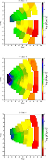 |
Fig. A.1. Density of M-giants with deconvolution of distance errors. Pixel size 1 × 1 (kpc); interpolation in X and Y directions up to 5 pixels. |
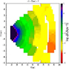 |
Fig. A.2. Density of M-giants without deconvolution correction (ρ0). Pixel size 1 × 1 (kpc); interpolation in X and Y directions up to 5 pixels. |
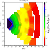 |
Fig. A.3. M-giant counts (Nparam.) per unit volume. Here, we show the density without correction of the selection effect or deconvolution. Pixel size 1 × 1 (kpc); interpolation in X and Y directions up to 5 pixels. |
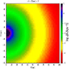 |
Fig. A.4. Prediction of [M/H] > −1.5 M-giants halo density from Fenkart (1989), with Q = 10.093, ρ⊙ = 2.5 × 10³ star/kpc3, and assuming that [M/H] > −1.5 stars are half of the total. |
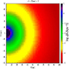 |
Fig. A.5. Prediction of [M/H] > −1.5 halo M-giants density from Xu et al. (2018), with n = 5.03, q = 1, AX, ⊙ = 1.4 × 10⁻³f ρ⊙, ρ⊙ = 2.5 × 10³ star/kpc3, and assuming that [M/H] > −1.5 stars are half of the total (f = 0.5). |
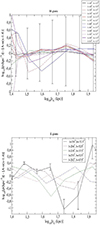 |
Fig. A.6. Residuals of the density given in Fig. 6 with respect to the linear fits for each line of sight (Table 1). Error bars (corresponding to the error of measured ρ0) of the first line of sight are plotted; for other lines of sight, the error bars are similar. |
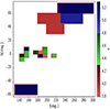 |
Fig. A.7. Variation of the power-law index n with the sky position in the 17 investigated lines of sight. |
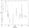 |
Fig. A.8. Power law index n vs. angular distance to the Sagittarius stream orbit ( |

All Tables
Best linear fits of the density profile in log–log, log10(ρ) = A − n(x − 1.40), x = log10[rG(kpc)], in the range log10[rG(kpc)] between 1.40 and 1.95 for the different lines of sight.
All Figures
|
Fig. 1. Sky distribution of LAMOST sources used in this paper: M-giants are colour-coded in black, K-giants in red. |
| In the text | |
|
Fig. 2. Luminosity function of our two samples. |
| In the text | |
|
Fig. 3. Absolute magnitude of the K-giant sources as a function of their heliocentric distance, and as a function of [Fe/H] for the subsample with r between 15 and 20 kpc. |
| In the text | |
|
Fig. 4. Stellar density as a function of heliocentric distance for M-giants (top panel; 40 973 sources) and K-giants (bottom panel; 19 521 sources). ρ0 is the observed density without correction of deconvolution or parallax errors; ρ is the density with deconvolution; ρL, [15] is the amount derived in Eq. (7), which converges to ρ0 after 15 iterations. |
| In the text | |
|
Fig. 5. Stellar density after deconvolution correction as a function of the distance to Galactic centre for M-giants (top panel; 40 973 sources) and K-giants (bottom panel; 19 521 sources). Error bars correspond to the Poissonian errors of the measured ρ0. |
| In the text | |
|
Fig. 6. Stellar density after deconvolution correction as a function of the distance to the Galactic centre. Upper panel: M-giants within 12 lines of sight with Δb = 5°, Δℓ = 10°. Bottom panel: K-giants within five lines of sight with Δb = 15°, Δℓ = 30 ° /cos(b). Fits correspond to the average of all lines of sight in the range log10[rG(kpc)] between 1.4 and 1.95, except the line ℓ = 154°, b = −52.5°, which presents an anomaly. Error bars (corresponding to the error of measured ρ0) of the first line of sight are plotted; for other lines of sight, the error bars are similar. |
| In the text | |
|
Fig. A.1. Density of M-giants with deconvolution of distance errors. Pixel size 1 × 1 (kpc); interpolation in X and Y directions up to 5 pixels. |
| In the text | |
|
Fig. A.2. Density of M-giants without deconvolution correction (ρ0). Pixel size 1 × 1 (kpc); interpolation in X and Y directions up to 5 pixels. |
| In the text | |
|
Fig. A.3. M-giant counts (Nparam.) per unit volume. Here, we show the density without correction of the selection effect or deconvolution. Pixel size 1 × 1 (kpc); interpolation in X and Y directions up to 5 pixels. |
| In the text | |
|
Fig. A.4. Prediction of [M/H] > −1.5 M-giants halo density from Fenkart (1989), with Q = 10.093, ρ⊙ = 2.5 × 10³ star/kpc3, and assuming that [M/H] > −1.5 stars are half of the total. |
| In the text | |
|
Fig. A.5. Prediction of [M/H] > −1.5 halo M-giants density from Xu et al. (2018), with n = 5.03, q = 1, AX, ⊙ = 1.4 × 10⁻³f ρ⊙, ρ⊙ = 2.5 × 10³ star/kpc3, and assuming that [M/H] > −1.5 stars are half of the total (f = 0.5). |
| In the text | |
|
Fig. A.6. Residuals of the density given in Fig. 6 with respect to the linear fits for each line of sight (Table 1). Error bars (corresponding to the error of measured ρ0) of the first line of sight are plotted; for other lines of sight, the error bars are similar. |
| In the text | |
|
Fig. A.7. Variation of the power-law index n with the sky position in the 17 investigated lines of sight. |
| In the text | |
|
Fig. A.8. Power law index n vs. angular distance to the Sagittarius stream orbit ( |
| In the text | |
Current usage metrics show cumulative count of Article Views (full-text article views including HTML views, PDF and ePub downloads, according to the available data) and Abstracts Views on Vision4Press platform.
Data correspond to usage on the plateform after 2015. The current usage metrics is available 48-96 hours after online publication and is updated daily on week days.
Initial download of the metrics may take a while.