Thermal tides in neutrally stratified atmospheres: Revisiting the Earth’s Precambrian rotational equilibrium

Mohammad Farhat; Pierre Auclair-Desrotour; Gwenaël Boué; Russell Deitrick; Jacques Laskar

doi:10.1051/0004-6361/202348625

Home

All issues

Volume 684 (April 2024)

A&A, 684 (2024) A49

Full HTML

Highlight

Open Access

Issue		A&A Volume 684, April 2024


Article Number		A49
Number of page(s)		23
Section		Planets and planetary systems
DOI		https://doi.org/10.1051/0004-6361/202348625
Published online		04 April 2024

A&A, 684, A49 (2024)

Thermal tides in neutrally stratified atmospheres: Revisiting the Earth’s Precambrian rotational equilibrium

Mohammad Farhat¹, Pierre Auclair-Desrotour¹, Gwenaël Boué¹, Russell Deitrick² and Jacques Laskar¹

¹ IMCCE, CNRS, Observatoire de Paris, PSL University, Sorbonne Université, 77 Avenue Denfert-Rochereau, 75014 Paris, France
e-mail: mohammad.farhat@obspm.fr
² School of Earth and Ocean Sciences, University of Victoria, Victoria, British Columbia, Canada

Received: 15 November 2023
Accepted: 15 January 2024

Abstract

Rotational dynamics of the Earth, over geological timescales, have profoundly affected local and global climatic evolution, probably contributing to the evolution of life. To better retrieve the Earth’s rotational history, and motivated by the published hypothesis of a stabilized length of day during the Precambrian, we examined the effect of thermal tides on the evolution of planetary rotational motion. The hypothesized scenario is contingent upon encountering a resonance in atmospheric Lamb waves, whereby an amplified thermotidal torque cancels out the opposing torque generated by the oceans and solid interior, driving the Earth into rotational equilibrium. With this scenario in mind, we constructed an ab initio model of thermal tides on rocky planets describing a neutrally stratified atmosphere. The model takes into account dissipative processes with Newtonian cooling and diffusive processes in the planetary boundary layer. We retrieved, from this model, a closed-form solution for the frequency-dependent tidal torque, which captures the main spectral features previously computed using 3D general circulation models. In particular, under longwave heating, diffusive processes near the surface and the delayed thermal response of the ground prove to be responsible for attenuating, and possibly annihilating, the accelerating effect of the thermotidal torque at the resonance. When applied to the Earth, our model prediction suggests the occurrence of the Lamb resonance in the Phanerozoic, but with an amplitude that is insufficient for the rotational equilibrium. Interestingly, though our study was motivated by the Earth’s history, the generic tidal solution can be straightforwardly and efficiently applied in exoplanetary settings.

Key words: Earth / planets and satellites: atmospheres / planets and satellites: dynamical evolution and stability / planets and satellites: terrestrial planets / planet–star interactions

© The Authors 2024

Open Access article, published by EDP Sciences, under the terms of the Creative Commons Attribution License (https://creativecommons.org/licenses/by/4.0), which permits unrestricted use, distribution, and reproduction in any medium, provided the original work is properly cited.

This article is published in open access under the Subscribe to Open model. Subscribe to A&A to support open access publication.

1 Introduction

For present-day Earth, the semi-diurnal atmospheric tide, driven by the thermal forcing of the Sun and generated via atmospheric pressure waves, describes the movement of atmospheric mass away from the substellar point. Consequently, mass culminates forming bulges on the nightside and the dayside, generating a torque that accelerates the Earth’s rotation. As such, this thermally generated torque counteracts the luni-solar gravitational torque associated with the Earth’s solid and oceanic tides. The latter components typically drive the closed system of the tidal players toward equilibrium states of orbital circularity, copla-narity, and synchronous rotation via dissipative mechanisms (e.g., Mignard 1980; Hut 1981). In contrast, the inclusion of the stellar flux as an external source of energy renders the system an open system where radiative energy is converted, by the atmosphere, into mechanical deformation and gravitational potential energy. Though this competition between the torques is established on Earth, the thermotidal torque remains, at least currently, orders of magnitude smaller.

Interestingly though, this dominance of the gravitational torque over the thermal counterpart admits exceptions. The question of the potential amplification of the atmospheric tidal response was initiated with Kelvin (1882), who invoked the theory of atmospheric tidal resonances, ushering a stream of theoretical studies investigating the normal modes’ spectrum of the Earth’s atmosphere (see Chapman & Lindzen 1970, for a neat and authoritative historical overview). Studies of the Earth’s tidal response spectrum advanced the theory of thermal tides for it to be applied to Venus (Goldreich & Soter 1966; Gold & Soter 1969; Ingersoll & Dobrovolskis 1978; Dobrovolskis & Ingersoll 1980; Correia & Laskar 2001, 2003b; Correia et al. 2003), hot Jupiters (e.g., Arras & Socrates 2010; Auclair-Desrotour & Leconte 2018; Gu et al. 2019; Lee 2020), and near-synchronous and Earth-like rocky exoplanets (Cunha et al. 2015; Leconte et al. 2015; Auclair-Desrotour et al. 2017a, Auclair-Desrotour et al. 2019). Namely, for planetary systems within the so-called habitable zone, the gravitational tidal torque diminishes in the regime near spin-orbit synchronization and becomes comparable in magnitude to the thermotidal torque. Consequently, the latter may actually prevent the planet from precisely reaching its destined synchronous state (Laskar & Correia 2004; Correia & Laskar 2010; Cunha et al. 2015; Leconte et al. 2015).

Going back to Earth, Holmberg (1952) suggested that the thermal tide at present is resonant, and the generated torque is equal in magnitude and opposite in sign to that generated by gravitational tides, thus placing the Earth into a rotational equilibrium with a stabilized spin rate. As this was proven to be untrue for the present Earth (Chapman & Lindzen 1970), Zahnle & Walker (1987) revived Holmberg’s hypothesis by applying the resonance scenario of thermal tides to the distant past. Their suggestion relied on two factors needed to close the gap between the competing torques. The first is the occurrence of a resonance in atmospheric Lamb waves (e.g., Lindzen & Blake 1972) – which we coin as a Lamb resonance – that characterizes the frequency overlap between the fundamental mode of atmospheric free oscillations and the semidiurnal forcing frequency. According to Zahnle & Walker (1987), this resonance occurred when the length of day (LOD) was around 21 h, exciting the thermotidal torque to large amplitudes. Secondly, the gravitational tidal torque must have been largely attenuated in the Precambrian. Recently, Bartlett & Stevenson (2016) revisited the equilibrium scenario and investigated the effect of temperature fluctuations on the stability of the resonance trapping and the Earth’s equilibrium. The authors concluded that the rotational stabilization could have lasted 1 billion years, only to be distorted by a drastic deglaciation event (on the scale that follows the termination of a snowball Earth), thus allowing the LOD to increase again from ~21 h to its present value. Evidently, the occurrence of such a scenario has very significant implications on paleoclimatic studies, with the growing evidence on links between the evolving LOD and the evolution of Precambrian benthic life (e.g., Klatt et al. 2021).

We are fresh out of a study on the tidal evolution of the Earth-Moon system (Farhat et al. 2022), where we focused on modeling tidal dissipation in the Earth’s paleo-oceans and solid interior. There we learned that the tidal response of the oceans, characterized by intermittent resonant excitations, is sufficient to explain the present rate of lunar recession and the estimated lunar age, and it is in good agreement with the geological proxies on the lunar distance and the LOD, leaving little to no place for an interval of a rotational equilibrium (Fig. 1).

On the other hand, major progress has been achieved in establishing the frequency spectrum of the thermotidal response of rocky planets with various approaches ranging from analytical models (Ingersoll & Dobrovolskis 1978; Dobrovolskis & Ingersoll 1980; Auclair-Desrotour et al. 2017a,b), to parameterized models that capture essential spectral features (e.g., Correia & Laskar 2001, 2003a), to fully numerical efforts that relied on the advancing sophistication of general circulation models (GCM; e.g., Leconte et al. 2015; Auclair-Desrotour et al. 2019). The latter work presents, to our knowledge, the first study to have numerically computed the planetary thermotidal torque in the high frequency regime, that is, around the Lamb resonance (Lindzen & Blake 1972). Of interest to us here are two perplexing results that Auclair-Desrotour et al. (2019) established: first, for planets near synchronization, the simplified Maxwellian models often used to characterize the thermotidal torque did not match the GCM simulated response; second, the torque at the Lamb resonance featured only a decelerating effect on the planet. Namely, it acts in the same direction of gravitational tides, and thus the effect required for the rotational stabilization disappeared.

More recently, two studies on the Precambrian LOD stabilization were published. Mitchell & Kirscher (2023) compiled various geological proxies on the Precambrian LOD and established the best piece-wise linear fit to this data compilation. The authors’ analysis depicts that a Precambrian LOD of 19 h was stabilized between 1 and 2 Ga. In parallel, Wu et al. (2023) also attempted to fit a fairly similar set of geological proxies, but using a simplified model of thermal tides. The authors conclude that the LOD was stabilized at ~19.5 h between 0.6 and 2.2 Ga, with a sustained very high mean surface temperature (40–55°C). Although using different approaches, the two studies have thus arrived at similar conclusions. A closer look at the subset of geological data that favored this outcome, however, indicates that both studies heavily rely on three stromatolitic records from the Paleoproterozoic that were originally studied by Pannella (1972a,b). These geological data have been, ever since, identified as unsuitable for precise quantitative interpretation (see e.g., Scrutton 1978; Lambeck 1980; Williams 2000). To this end, we provide a more detailed analysis of the geological proxies of the LOD, and of the model presented by Wu et al. (2023) in a parallel paper dedicated to the matter (Laskar et al. 2023).

With a view to greater physical realism, we aim here to study, analytically, the frequency spectrum of the thermotidal torque, from first principles, interpolating between the low and high frequency regimes. Our motivation is two-fold: first, to provide a novel physical model for the planetary thermotidal torque that better matches the GCM-computed response, and that can be used in planetary dynamical evolution studies; second, to apply this model to the Earth and attempt quantifying the amplitude of the torque at the Lamb resonance and explore the intriguing rotational equilibrium scenario.

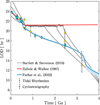Fig. 1

Modeled histories of the rotational motion of the Earth. The Earth’s LOD evolution is plotted in time over geological timescales for three models: (i) the model of Farhat et al. (2022), where the evolution is driven solely by oceanic and solid tidal dissipation; and (ii) the model of Zahnle & Walker (1987), where the Lamb resonance is encountered for LOD~21 h, forcing a rotational equilibrium on the Earth; (iii) the model of Bartlett & Stevenson (2016), which also adopts the equilibrium scenario, but further studies the effect of thermal noise, and the required temperature variation to escape the equilibrium. Three curves of the latter model correspond to different parameterizations of the gravitational tide. Plotted on top of the modeled histories are geological proxies of the LOD evolution which can be retrieved from http://astrogeo.eu.

2 Ab initio atmospheric dynamics

For an atmosphere enveloping a spherically symmetric planet, we define a reference frame corotating with the planet. In this frame, an atmospheric parcel is traced by its position vector r in spherical coordinates (r, θ, φ), such that θ is the colatitude, φ is the longitude, and the radial distance |r| = R_p + z, where R_p is the planet’s radius and z is the parcel’s atmospheric altitude. The atmosphere is characterized by the scalar fields of pressure p, temperature T, density ρ, and the three-dimensional vectorial velocity field 𝒱. Each of these fields varies in time and space, and is decomposed linearly into two terms: a background, equilibrium state field, subscripted with 0, and a tidally forced perturbation term of significantly smaller amplitude such that p = p₀ + δp, T = T₀ + δT, ρ = ρ₀ + δρ, and 𝒱 = V₀ + V.

Our fiducial atmosphere is subject to the perturbative gravitational tidal potential U and the thermal forcing per unit mass J. We shall define the latter component precisely in Sect. 2.2, but for now it suffices to say that J accounts for the net amount of heat, per unit mass, provided to the atmosphere, allowing for thermal losses driven by radiative dissipation. We take the latter effect into account by following the linear Newtonian cooling hypothesis¹ (Lindzen & McKenzie 1967), where radiative losses, J_rad, are parameterized by the characteristic frequency σ₀; namely J_rad = p₀σ₀/(κρ₀T₀)δT, where κ = (Γ₁ − 1)/Γ₁ = 0.285 and Γ₁ is the adiabatic exponent. Similar to Leconte et al. (2015), we associate with σ₀ a radiative cooling timescale τ_rad = 4τ/σ0.

2.1 The vertical structure of tidal dynamics

We are interested in providing a closed-form solution for the frequency² dependence of the thermotidal torque, which results from tidally driven atmospheric mass redistribution. By virtue of the hydrostatic approximation, this mass redistribution is encoded in the vertical profile of pressure. As such, it is required to solve for the vertical structure of tidal dynamics. With fellow non-theoreticians in mind, we delegate the detailed development of the governing system of equations describing the tidal response of the atmosphere to Appendix A. Therein, we employ the classical system of primitive equations describing momentum and mass conservation (e.g., Siebert 1961; Chapman & Lindzen 1970), atmospheric heat transfer augmented with linear radiative transfer à la Lindzen & McKenzie (1967), and the ideal gas law, all formulated in a dimensionless form.

Aided by the so-called traditional approximation (e.g., Unno et al. 1979, see also Appendix A), the analytical treatment of the said system is feasible as it decomposes into two parts describing, separately, the horizontal and vertical structures of tidal flows. The former part is completely described by the eigenvalue-eigenfunction problem defined as Laplace’s tidal equation (Laplace 1798; Lee & Saio 1997):

$ℒ^{m, v} Θ_{n}^{m, v} = - Λ_{n}^{m, v} Θ_{n}^{m, v},$ ${{\cal L}^{m,v}}{\rm{\Theta }}_n^{m,v} = - {\rm{\Lambda }}_n^{m,v}{\rm{\Theta }}_n^{m,v},$ (1)

where the set of Hough functions ${Θ_{n}^{m, v}}$ $\left\{ {{\rm{\Theta }}_n^{m,v}} \right\}$ serves as the solution (Hough 1898), ${Λ_{n}^{m, v}}$ $\left\{ {{\rm{\Lambda }}_n^{m,v}} \right\}$ is the associated set of eigenvalues, ℒ^m,v is a horizontal operator defined in Eq. (A.23), while v = 2Ω/σ, where Ω is the rotational velocity of the planet and σ is the tidal forcing frequency. In the tidal system under study, the variables and functions (δp, δρ, δT, V, J, Θ, Λ) are written in the Fourier domain using the longitudinal order m and frequency σ (Eq. (A.20)), and expanded in horizontal Hough modes with index n (Eq. (A.21)). We denote hereafter their coefficients $f_{n}^{m, v}$ $f_n^{m,v}$ by f_n to lighten the expressions. This horizontal structure of tidal dynamics is merely coupled to the vertical structure via the set of eigenvalues ${Λ_{n}^{m, v}}$ $\left\{ {{\rm{\Lambda }}_n^{m,v}} \right\}$ . To construct these sets of eigenfunctions-eigenvalues we use the spectral method laid out by Wang et al. (2016).

The vertical structure on the other hand requires a more elaborate manipulation of the governing system, a procedure that we detail in Appendix B. The outcome is a wave-like equation that describes vertical thermotidal dynamics and reads as:

$\frac{d^{2} Ψ_{n}}{d x^{2}} + {\hat{k}}_{n}^{2} Ψ_{n} = Φ^{- 1} C_{n} .$ ${{{{\rm{d}}^2}{{\rm{\Psi }}_n}} \over {{\rm{d}}{x^2}}} + \hat k_n^2{{\rm{\Psi }}_n} = {{\rm{\Phi }}^{ - 1}}{C_n}.$ (2)

Here, as is the common practice (e.g., Siebert 1961; Chapman & Lindzen 1970), we use the reduced altitude $x = {\int^{}}_{0}^{z} d z / H (z)$ $x = \mathop \smallint \nolimits^ _0^z\,{\rm{d}}z/H(z)$ as the vertical coordinate, where the pressure scale height H(z) = ℛ_sT₀(z)/g, with ℛ_s being the specific gas constant and g the gravitational acceleration. The quantity Ψ_n(x) is a calculation variable from which, once solved for, all the tidal scalar and vectorial quantities would flesh out (Appendix C). The vertical wave number ${\hat{k}}_{n} (x)$ ${{\hat k}_n}(x)$ is defined via

$\begin{array}{l} {\hat{k}}_{n}^{2} (x) = - \frac{1}{4} {{(1 - \frac{i κ}{α - i} (γ - 1))}^{2} + 2 \frac{d}{d x} (\frac{i γ}{α - i}) \\ - \frac{4 α κ}{α - i} [β γ Λ_{n} - \frac{i}{α} (γ - 1)]} . \end{array}$ $\matrix{ {\hat k_n^2(x) = - {1 \over 4}\left\{ {{{\left( {1 - {{i\kappa } \over {\alpha - i}}(\gamma - 1)} \right)}^2} + 2{{\rm{d}} \over {{\rm{d}}x}}\left( {{{i\gamma } \over {\alpha - i}}} \right)} \right.} \hfill \cr {\left. {\,\,\,\,\,\,\,\,\,\,\,\,\,\,\,\,\,\,\,\, - {{4\alpha \kappa } \over {\alpha - i}}\left[ {\beta \gamma {{\rm{\Lambda }}_n} - {i \over \alpha }(\gamma - 1)} \right]} \right\}.} \hfill \cr }$ (3)

By virtue of the non-dimensionalization of the governing system of equations, dimensionless control parameters appear in the wavenumber definition. Namely, $α = σ / σ_{0}, β = σ_{w}^{2} / σ^{2}$ $\alpha = \sigma /{\sigma _0},\beta = \sigma _{\rm{w}}^2/{\sigma ^2}$ , and $γ = N_{B}^{2} / N_{B; iso}^{2}$ $\gamma = N_{\rm{B}}^2/N_{{\rm{B}};{\rm{iso}}}^2$ , where we have introduced the characteristic frequency $σ_{w} = \sqrt{g H} / R_{p}$ ${\sigma _{\rm{w}}} = \sqrt {gH} /{R_{\rm{p}}}$ , a typical frequency of Lamb waves. Of significance to the computations that follow is the Brunt–Väisälä frequency, N_B, a measure of the vertical density stratification of the atmosphere against the strength of convection (e.g., Vallis 2017). Under hydrostatic equilibrium, N_B is defined as:

$N_{B}^{2} = \frac{g}{H} (κ + \frac{d \ln H}{dx}) .$ $N_{\rm{B}}^2 = {g \over H}\left( {\kappa + {{{\rm{d}}\ln {\rm{H}}} \over {{\rm{dx}}}}} \right).$ (4)

We define the Brunt–Väisälä frequency in the limit of an isothermal atmospheric profile, $N_{B; iso} = \sqrt{κ g / H}$ ${N_{{\rm{B}};{\rm{iso}}}} = \sqrt {\kappa g/H}$ . As such, the parameter γ measures the local atmospheric stability against convection with respect to the stability of an equivalent isothermal atmosphere. These key control parameters, among others, qualitatively determine the regime of the tidal response. We summarize these parameters in Table 1. The right hand side of the wave Eq. (2) combines the function Φ defined as

$Φ (x) = \exp [\frac{x}{2} - \frac{1}{2} {\int^{}}_{0}^{x} \frac{i}{α - i} (\frac{H N_{B}^{2}}{g} - κ) d x^{'}],$ ${\rm{\Phi }}(x) = \exp \left[ {{x \over 2} - {1 \over 2}\mathop \smallint \nolimits^ _0^x{i \over {\alpha - i}}\left( {{{HN_{\rm{B}}^2} \over g} - \kappa } \right){\rm{d}}x'} \right],$ (5)

and the forcing function C_n(x) which reads:

$C_{n} (x) = \frac{α β Λ_{n} {\tilde{J}}_{n}}{α - i} + [\frac{κ (γ - 1)}{α - i} (Λ_{n} + \frac{\partial_{x}}{β}) - i \partial_{x} (\frac{\partial_{x}}{β})] {\tilde{U}}_{n} .$ ${C_n}(x) = {{\alpha \beta {{\rm{\Lambda }}_n}{{\tilde J}_n}} \over {\alpha - i}} + \left[ {{{\kappa (\gamma - 1)} \over {\alpha - i}}\left( {{{\rm{\Lambda }}_n} + {{{\partial _x}} \over \beta }} \right) - i{\partial _x}\left( {{{{\partial _x}} \over \beta }} \right)} \right]{\tilde U_n}.$ (6)

Hereafter, we identify the dimensionless form of the tidal variables by the tilde diacritic. Namely in Eq. (6), the dimensionless thermal forcing function ${\tilde{J}}_{n} = κ / (g σ H) J_{n}$ ${{\tilde J}_n} = \kappa /(g\sigma H){J_n}$ , while the gravitational analog ${\tilde{U}}_{n} = U_{n} / v_{0}^{2}$ ${{\tilde U}_n} = {U_n}/v_0^2$ , where the reference velocity $v_{0} = σ R_{p}$ ${v_0} = \sigma {R_{\rm{p}}}$ (see Eq. (A.11) for the rest of the dimensionless quantities). As we intend to solve the wave equation in the following sections, what is left for us to quantify the mass redistribution and compute the resulting tidal torque is to retrieve the vertical profile of pressure given the solution of the wave equation, Ψ_n(x). In Appendix C, we derive the vertical profiles of all the tidal variables, and specifically for the dimensionless pressure anomaly we obtain:

$\tilde{δ} p_{n} (x) = \frac{1}{i β Λ_{n}} (\frac{d {\tilde{G}}_{n}}{d x} - {\tilde{G}}_{n}) + \frac{1}{β} (1 + \frac{1}{β Λ_{n}} \frac{d}{dx}) {\tilde{U}}_{n},$ $\widetilde \delta {p_n}(x) = {1 \over {i\beta {{\rm{\Lambda }}_n}}}\left( {{{{\rm{d}}{{\tilde G}_n}} \over {{\rm{d}}x}} - {{\tilde G}_n}} \right) + {1 \over \beta }\left( {1 + {1 \over {\beta {{\rm{\Lambda }}_n}}}{{\rm{d}} \over {{\rm{dx}}}}} \right){\tilde U_n},$ (7)

where $\tilde{δ} p_{n} (x) = δ p_{n} (x) / p_{0}$ $\tilde \delta {p_n}\,(x) = \delta {p_n}(x)/{p_0}$ , and the calculation variable $\tilde{G} n (x) = Ψ_{n} (x) Φ (x)$ $\tilde Gn(x) = {{\rm{\Psi }}_n}(x){\rm{\Phi }}(x)$ .

Table 1

Dimensionless control parameters determining the regime of the atmospheric tidal response and defined throughout the text.

2.2 The thermal forcing profile

To solve the nonhomogeneous wave Eq. (2), it is necessary to define a vertical profile for the tidal heating power per unit mass ${\tilde{J}}_{n}$ ${{\tilde J}_n}$ (or equivalently in dimensional form, J_n). We adopt a vertical tidal heating profile of the form

$J_{n} (x) = J_{s} e^{- b_{J} x},$ ${J_n}(x) = {J_{\rm{s}}}{{\rm{e}}^{ - {b_{\rm{J}}}x}},$ (8)

where J_s is the heat absorbed at the surface and b_J is a decay rate that characterizes the exponential decay of heating along the vertical coordinate. As we are after a generic planetary model, this functional form of J_n allows the distribution of heat to vary between the Dirac distribution adopted by Dobrovolskis & Ingersoll (1980) where b_J → ∞, and a uniform distribution where the whole air column is uniformly heated (b_J = 0).

To determine J_s, we invoke its dependence on the total vertically propagating flux δF_tot by computing the energy budget over the air column. The net input of energy corresponds to the difference between the amount of flux absorbed by the column and associated with a local increase of thermal energy, and the amount that escapes into space or into the mean flows defining the background profiles. We quantify the fraction of energy transferred to the atmosphere and that is available for tidal dynamics by α_A, where 0 ≤ α_A ≤ 1; the rest of the flux amounting to 1 − α_A escapes the thermotidal interplay. We thus have

${\int^{}}_{0}^{\infty} J (x) ρ_{0} (x) H (x) dx = α_{A} δ F_{tot} .$ $\mathop \smallint \nolimits^ _0^\infty J(x){\rho _0}(x)H(x){\rm{dx}} = {\alpha _{\rm{A}}}\delta {{\rm{F}}_{{\rm{tot}}}}.$ (9)

To define δF_tot, we establish the flux budget for a small thermal perturbation at the planetary surface. We start with δF_inc, a variation of the effective incident stellar flux, after the reflected component has been removed. δF_inc generates a variation δT_s in the surface temperature T_s. The proportionality between δF_inc and δT_s is parameterized by τ_bl, a characteristic diffusion timescale of the ground and atmospheric surface thermal responses. We detail on this proportionality in Appendix D, but for now it suffices to state that τ_bl is a function of the thermal inertia budgets in the ground, I_gr, and the atmosphere I_atm.

We associate with τ_bl the frequency $σ_{bl} = τ_{bl}^{- 1}$ ${\sigma _{{\rm{bl}}}} = \tau _{{\rm{bl}}}^{ - 1}$ , a characteristic frequency that reflects the thermal properties of the diffusive boundary layer. It will serve as another free parameter of our tidal model, besides the Newtonian cooling frequency σ₀, and the atmospheric opacity parameter α_A. In analogy to a = σ/σ₀ we define the dimensionless parameter for the boundary layer $ζ = \sqrt{| σ | τ_{b 1}} = \sqrt{| σ | / σ_{bl}}$ $\zeta = \sqrt {|\sigma |{\tau _{{\rm{b}}1}}} = \sqrt {|\sigma |/{\sigma _{{\rm{bl}}}}}$ .

By virtue of the power budget balance established in Appendix D, we define the total propagating flux δF_tot as

$δ F_{tot} = δ F_{inc} [1 - μ_{gr} ζ \frac{1 + s i}{1 + (1 + s i) ζ}] .$ $\delta {F_{{\rm{tot}}}} = \delta {F_{{\rm{inc}}}}\left[ {1 - {\mu _{{\rm{gr}}}}\zeta {{1 + si} \over {1 + (1 + si)\zeta }}} \right].$ (10)

Here, s = sign(σ), and µ_gr is a dimensionless characteristic function weighing the relative contribution of ground thermal inertia to the total inertia budget; namely µ_gr = I_gr/(I_gr + I_atm).

The generic form of the flux in Eq. (10) clearly depicts two asymptotic regimes of thermotidal forcing:

(i)
Ignoring the surface layer effects associated with the term on the right, that is, setting ζ = µ_gr = 0, leaves us with ther-motidal heating that is purely attributed to the direct atmospheric absorption of the incident flux. This limit can be used to describe the present understanding of thermotidal forcing on Earth where, to first order, direct insolation absorption in the shortwave by ozone and water vapor appears sufficient to explain the observed tidal amplitudes in barometric measurements (e.g., Chapman & Lindzen 1970; Schindelegger & Ray 2014). Nevertheless, it is noteworthy that the observed tidal phases of pressure maxima could not be explained by this direct absorption, a discrepancy later attributed to an additional semidiurnal forcing, namely that of latent heat release associated with cloud and raindrop formation (e.g., Lindzen 1978; Hagan & Forbes 2002; Sakazaki et al. 2017).
(ii)
Allowing for the surface layer term on the other hand (ζ ≠ 0, µ_gr ≠ 0) places us in the limit where the ground radiation in the infrared and heat exchange processes occurring in the vicinity of the surface would dominate the thermotidal heating. The total tidal forcing in this case is nonsynchronous with the incident flux due to the delayed thermal response of the ground, which here is a function of τ_bl. This limit better describes dry Venus-like planets, as is the fiducial setting studied using GCMs in Leconte et al. (2015) and Auclair-Desrotour et al. (2019).

Finally, as we are interested in the semi-diurnal tidal response, we decompose the thermal forcing in Appendix E to obtain the amplitude of the quadrupolar component as $δ F_{inc} = δ F_{22} = (\sqrt{30 π} / 16) F_{⋆}$ $\delta {F_{{\rm{inc}}}} = \delta {F_{22}} = (\sqrt {30\pi } /16){F_ \star }$ , where $F_{⋆} = L_{⋆} / 4 π a_{p}^{2}, L_{⋆}$ ${F_ \star } = {L_ \star }/4\pi a_{\rm{p}}^2,{L_ \star }$ , L_⋆ being the stellar luminosity, and a_p the star-planet distance.

3 The tidal response

3.1 The tidal torque in the neutral stratification limit

Under the defined forcing in the previous section, to solve the wave equation analytically, a choice has to be made on the Brunt–Väisälä frequency, N_B (Eq. (4)), which describes the strength of atmospheric buoyancy forces and consequently the resulting vertical temperature profile. Earlier analytical solutions have been obtained in the limit of an isothermal atmosphere (Lindzen & McKenzie 1967; Auclair-Desrotour et al. 2019), in which case the scale height H becomes independent of the vertical coordinate, and by virtue of Eq. (4), 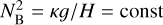$N_{B}^{2} = κ g / H = const$ $N_{\rm{B}}^2 = \kappa g/H = {\rm{const}}$ .

Motivated by the Earth’s atmosphere, where the massive troposphere (~80% of atmospheric mass) controls the tidal mass redistribution, we derive next an analytical solution in a different, and perhaps more realistic limit. Namely, the limit corresponding to the case of a neutrally stratified atmosphere, where $N_{B}^{2} = 0$ $N_{\rm{B}}^2 = 0$ . In fact, $N_{B}^{2}$ $N_{\rm{B}}^2$ can be expressed in terms of the potential temperature Θ₀ (e.g., Sect. 2.10 of Vallis 2017):

$N_{B}^{2} = \frac{g}{H} \frac{d \ln Θ_{0}}{dx},$ $N_{\rm{B}}^2 = {g \over H}{{{\rm{d}}\ln {{\rm{\Theta }}_0}} \over {{\rm{dx}}}},$ (11)

whereby the stability of the atmosphere is controlled by the slope of Θ₀. To this end, atmospheric temperature measurements (e.g., Figs. 2.1–2.3 of Pierrehumbert 2010) clearly depict that the troposphere is characterized by a negative temperature gradient, and a weak potential temperature gradient, which is closer to an idealized adiabatic profile than it is to an idealized isothermal profile. Moreover, the heating in the troposphere generates strong convection and efficient turbulent stirring, thus enhancing energy transfer and driving the layer toward an adiabatic temperature profile, away from the isothermal profile. Consequently, the adiabatic temperature profile prohibits the propagation of buoyancy-restored gravity waves, which compose the baroclinic component of the atmospheric tidal response (e.g., Gerkema & Zimmerman 2008). This leaves the atmosphere with the barotropic component of the tidal flow, a feature that is consistent with tidal dynamics under the shallow water approximation (Appendix A).

Hereafter, we focus on the thermotidal heating as the only tidal perturber, and we ignore the much weaker gravitational potential Ũ. It follows, in the neutral stratification limit, that γ = 0 (Table 1), and the vertical wavenumber (Eq. (3)) reduces to³

${\hat{k}}^{2} = {[\frac{1 + κ + i α}{2 (α - i)}]}^{2} .$ ${\hat k^2} = {\left[ {{{1 + \kappa + i\alpha } \over {2(\alpha - i)}}} \right]^2}.$ (12)

It also follows that the background profiles of the scalar variables read as (Auclair-Desrotour et al. 2017a):

$\begin{array}{l} p_{0} (x) = p_{0} (0) e^{- x}, ρ_{0} (x) = \frac{p_{0} (0)}{g H (0)} e^{(κ - 1) x}, \\ T_{0} (x) = \frac{g H (0)}{ℛ_{s}} e^{- κ x} . \end{array}$ $\matrix{ {{p_0}(x) = {p_0}(0){e^{ - x}},\quad {\rho _0}(x) = {{{p_0}(0)} \over {gH(0)}}{e^{(\kappa - 1)x}},} \hfill \cr {{T_0}(x) = {{gH(0)} \over {{{\cal R}_{\rm{s}}}}}{{\rm{e}}^{ - \kappa x}}.} \hfill \cr }$ (13)

We thus obtain for the heating profile (using Eqs. (8), (9), and (10))

$J_{s} = δ F_{22} \frac{α_{A} g (b_{J} + 1)}{p_{0} (0)} [1 - μ_{gr} ζ \frac{1 + s i}{1 + (1 + s i) ζ}] .$ ${J_{\rm{s}}} = \delta {F_{22}}{{{\alpha _{\rm{A}}}g\left( {{b_{\rm{J}}} + 1} \right)} \over {{p_0}(0)}}\left[ {1 - {\mu _{{\rm{gr}}}}\zeta {{1 + si} \over {1 + (1 + si)\zeta }}} \right].$ (14)

As such, the wave Eq. (2) is rewritten as

$\frac{d^{2} Ψ_{n}}{{dx}^{2}} + {\hat{k}}^{2} Ψ_{n} = 𝒜_{n} e^{- ℬ x},$ ${{{{\rm{d}}^2}{{\rm{\Psi }}_{\rm{n}}}} \over {{\rm{d}}{{\rm{x}}^2}}} + {\hat k^2}{{\rm{\Psi }}_n} = {{\cal A}_n}{{\rm{e}}^{ - {\cal B}x}},$ (15)

where the complex functions 𝒜_n and ℬ are defined as:

$𝒜_{n} = \frac{κ Λ_{n}}{R_{p}^{2} σ^{3}} \frac{α^{2} + i α}{α^{2} + 1} J_{s},$ ${{\cal A}_n} = {{\kappa {{\rm{\Lambda }}_n}} \over {R_{\rm{p}}^2{\sigma ^3}}}{{{\alpha ^2} + i\alpha } \over {{\alpha ^2} + 1}}{J_{\rm{s}}}{\rm{,}}$ (16) $ℬ = \frac{1}{2 (α^{2} + 1)} [(2 b_{J} + 1) (α^{2} + 1) - κ + i κ α] .$ ${\cal B} = {1 \over {2\left( {{\alpha ^2} + 1} \right)}}\left[ {\left( {2{b_{\rm{J}}} + 1} \right)\left( {{\alpha ^2} + 1} \right) - \kappa + i\kappa \alpha } \right].$ (17)

The wave Eq. (15) admits the general solution

$Ψ_{n} (x) = c_{1} e^{i \hat{k} x} + c_{2} e^{- i \hat{k} x} + \frac{𝒜_{n}}{ℬ^{2} + {\hat{k}}^{2}} e^{- ℬ x} .$ ${{\rm{\Psi }}_n}\left( x \right) = {c_1}{{\rm{e}}^{i\hat kx}} + {c_2}{{\rm{e}}^{ - i\hat kx}} + {{{{\cal A}_n}} \over {{{\cal B}^2} + {{\hat k}^2}}}{{\rm{e}}^{ - {\cal B}x}}.$ (18)

We consider the following two boundary conditions:

– First, the energy of tidal flows, 𝒲, should be bounded as x → ∞. In Appendix F, we derive the expression of the tidal energy following Wilkes (1949), and it scales as $W \propto | Ψ |^{2} | Φ |^{2}$ ${\cal W} \propto |{\rm{\Psi }}{|^2}|{\rm{\Phi }}{|^2}$ . Accordingly, the non-divergence of the flow condition is satisfied if one sets c₂ = 0 and takes the proper sign of the wavenumber (Eq. (12)), namely:

$\hat{k} = \frac{1}{2 (α^{2} + 1)} [κ α + i (1 + κ + α^{2})] .$ $\hat k = {1 \over {2\left( {{\alpha ^2} + 1} \right)}}\left[ {\kappa \alpha + i\left( {1 + \kappa + {\alpha ^2}} \right)} \right].$ (19)

– The second condition is the natural wall condition imposed by the ground interface, which enforces ${\tilde{V}}_{r; n} (x = 0) = 0$ ${{\tilde V}_{r;n}}(x = 0) = 0$ . We derive the expression of the profile of the vertical velocity in Appendix C, and by virtue of Eq. (C.6), this condition allows us to write c₁ in the form:

$c_{1} (x) = \frac{𝒜_{n}}{ℬ + {\hat{k}}^{2}} \times \frac{ℬ - \frac{1}{2} (1 + \frac{i κ}{α - i}) - β Λ_{n} + 1}{i \hat{k} + \frac{1}{2} (1 + \frac{i κ}{α - i}) + β Λ_{n} - 1} .$ ${c_1}\left( x \right) = {{{{\cal A}_n}} \over {{\cal B} + {{\hat k}^2}}} \times {{{\cal B} - {1 \over 2}\left( {1 + {{i\kappa } \over {\alpha - i}}} \right) - \beta {{\rm{\Lambda }}_n} + 1} \over {i\hat k + {1 \over 2}\left( {1 + {{i\kappa } \over {\alpha - i}}} \right) + \beta {{\rm{\Lambda }}_n} - 1}}.$ (20)

Under these boundary conditions, we are now fully geared to analytically compute the solution of the wave equation, Ψ_n(x) (or equivalently ${\tilde{G}}_{n} (x)$ ${{\tilde G}_n}(x)$ ), but we are specifically interested in retrieving a closed-form solution of the quadrupolar tidal torque. The latter takes the general form⁴ (Appendix G):

$𝒯 = \sqrt{\frac{6 π}{5}} \frac{M_{⋆}}{M_{p}} \frac{R_{p}^{6}}{a_{p}^{3}} Im {δ p_{s}} .$ ${\cal T} = \sqrt {{{6\pi } \over 5}} {{{M_ \star }} \over {{M_{\rm{p}}}}}{{R_{\rm{p}}^6} \over {a_{\rm{p}}^3}}{\rm{Im}}\left\{ {\delta {p_{\rm{s}}}} \right\}.$ (21)

Here M_⋆ and M_p designate the stellar and planetary masses respectively, and Im refers to the imaginary part of a complex number, the latter in this case being the quadrupolar pressure anomaly at the surface $δ p_{s} = δ p_{2}^{2, v} (x = 0)$ $\delta {p_{\rm{s}}} = \delta p_2^{2,v}(x = 0)$ . We further note that while this torque is computed for the atmosphere, it does act on the whole planet since the atmosphere is a thin layer that features no differential rotation with respect to the rest of the planet.

Taking the solution Ψ(0) of Eq. (18) (with c₂ = 0 and c₁ defined in Eq. (20)), we retrieve δp_s from Eq. (7). After straightforward, but rather tedious manipulations, we extract the imaginary part of the pressure anomaly and write it in the simplified form:

$\begin{array}{l} Im {δ p_{s}} = α_{A} δ F_{22} \frac{κ g Λ_{2}}{R_{p}^{2} σ^{3}} \frac{(𝒳 α + 𝒴) α}{(1 + 2 ζ + 2 ζ^{2})} \\ \times \underset{position of the Lamb resonance}{\underset{︸}{{[{(κ - β Λ_{2} + 1)}^{2} + α^{2} {(β Λ_{2} - 1)}^{2}]}^{- 1}}}, \end{array}$ $\matrix{ {{\rm{Im}}\left\{ {\delta {p_{\rm{s}}}} \right\} = {\alpha _{\rm{A}}}\delta {F_{22}}{{\kappa g{{\rm{\Lambda }}_2}} \over {R_{\rm{p}}^2{\sigma ^3}}}{{\left( {X\alpha + Y} \right)\alpha } \over {\left( {1 + 2\zeta + 2{\zeta ^2}} \right)}}} \hfill \cr {\,\,\,\,\,\,\,\,\,\,\,\,\,\,\,\,\,\,\,\,\,\,\,\,\,\,\,\, \times \underbrace {{{\left[ {{{\left( {\kappa - \beta {{\rm{\Lambda }}_2} + 1} \right)}^2} + {\alpha ^2}{{\left( {\beta {{\rm{\Lambda }}_2} - 1} \right)}^2}} \right]}^{ - 1}}}_{{\rm{position of the Lamb resonance}}},} \hfill \cr }$ (22)

where we have defined the complex functions 𝒳 and 𝒴 as

$\begin{array}{l} 𝒳 = (β Λ_{2} - 1) [2 ζ^{2} (1 - μ_{gr}) + ζ (2 - μ_{gr}) + 1], \\ 𝒴 = - s μ_{gr} ζ (κ - β Λ_{2} + 1) . \end{array}$ $\matrix{ {X = \left( {\beta {{\rm{\Lambda }}_2} - 1} \right)\left[ {2{\zeta ^2}\left( {1 - {\mu _{{\rm{gr}}}}} \right) + \zeta \left( {2 - {\mu _{{\rm{gr}}}}} \right) + 1} \right],} \hfill \cr {\,Y = - s{\mu _{{\rm{gr}}}}\zeta \left( {\kappa - \beta {{\rm{\Lambda }}_2} + 1} \right).} \hfill \cr }$ (23)

We note that we provide the full complex transfer function of the surface pressure anomaly, along with further analysis on its functional form in Appendix H. In Appendix I, we show that the same form of the tidal solution given by Eq. (22) holds for moist and dry adiabatic profiles, subject to interchanging few effective parameters by their humidity-dependent analogs.

Before embarking on any results, we pause here for a few remarks on the provided closed-form solution of the torque.

The parameter α_A, defined earlier (Eq. (9)) as the fraction of radiation actually absorbed by the atmosphere, can evidently be correlated with the typical transmission function of the atmosphere and therefore its optical depth. Presuming that ther-motidal heating on Earth is driven by ozone and water vapor, α_A can then characterize atmospheric opacity parameter in the visible. Explicitly showing this dependence now takes us too far afield, though we compute and infer estimates of α_A in Sect. 4.1 and Appendix J.
The quadrupolar component of the equilibrium stellar flux, entering through a fraction of F_⋆ (Appendix E), is directly proportional to the stellar luminosity L_⋆. Standard models suggest that the Sun’s luminosity was around 80% of its present value ~3 Ga (Gough 1981). Such luminosity evolution of Sun-like stars can be directly accommodated in the model if one were to study the evolution of the tidal torque with time.
As we mentioned earlier, upon separating the horizontal and vertical structure of tidal dynamics, the only remaining coupling factor between the two structures is the eigenvalue of horizontal flows, A_n, which reduces in our case to the dominant fundamental mode Λ₂. Noting that we have dropped the superscripts, we remind the reader that for the semidiurnal (m = 2) response, $Λ_{2} = Λ_{2}^{2, v}$ ${{\rm{\Lambda }}_2} = {\rm{\Lambda }}_2^{2,v}$ , thus A is frequency-dependent in the general case. The Earth however, over its lifetime, lives in the asymptotic regime of v ≈ 1 since 2Ω ≫ n_⋆, thus it is safe to assume that Λ₂ is invariant over the geological history with a value of 11.159 that we compute using the spectral method of Wang et al. (2016).
Of significance to us in the Precambrian rotational equilibrium hypothesis is the tidal frequency, and consequently the LOD, at which the Lamb resonance occurs. It is evident from the closed-form solution (Eq. (22)) that the position of the resonance is controlled by the highlighted term. Had it not been for the introduced radiative losses, entering here through a, this term would have encountered a singularity at the spectral position of the resonance, namely for βΛ₂ = 1. Here, however, the amplitude of the tidal peak is finite, and its position is a function of the planetary radius, gravitational acceleration, average surface temperature, eigenvalue of the fundamental Hough mode of horizontal flows, and the Newtonian cooling frequency. We detail further on this dependence in Sect. 4.2.

In Fig. 2, we plot the spectrum of the tidal response for a fiducial system in terms of the normalized surface pressure anomaly over a wide range of tidal frequencies covering the low and high frequency regimes. The system describes a Venus-like dry planet (M_p = 0.815M_⊕, R_p = 0.95 R_⊕, a_p = 0.73 au, g = 8.87 m s⁻²), with a 10 bar atmosphere and a scale height at the surface H₀ = 10 km, thermally forced by a solar-like star (M_⋆ = 1 M_⊙, L_⋆ = 1 L_⊙). We further ignore here the thermal inertia in the ground and the atmosphere by taking σ_bl → ∞, or ζ → 0, thus assuming an synchronous response of the ground with the thermal excitation.

Key tidal response features are recovered in this spectrum: first, we obtain a tidal peak near synchronization (ω = 0) that generates a positive torque for σ > 0 and a negative torque for σ < 0, driving the planet in both cases away from its destined spin-orbit synchronization due to the effect of solid tides (e.g., Gold & Soter 1969; Correia & Laskar 2001; Leconte et al. 2015). The peak has often been modeled by a Maxwellian functional form, though this form does not always capture GCM-generated spectra when varying the planetary setup (e.g., Auclair-Desrotour et al. 2019). Second, we recover the Lamb resonance in the high frequency regime. The resonance is characterized here by two symmetric peaks of opposite signs. Thus upon passage through the resonance, the thermotidal torque shifts from being a rotational brake to being a rotational pump. In this work, we are more interested in the high frequency regime, thus we delegate further discussion and analysis on the low frequency tidal response to a forthcoming work, and we focus next on the Lamb resonance.

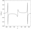Fig. 2

Spectrum of semi-diurnal atmospheric thermal tides. Plotted is the imaginary part of the normalized pressure anomaly ( ${\tilde{δ}}_{p} = δ p / p_{s}$ ${{\tilde \delta }_p} = \delta p/{p_{\rm{s}}}$ ; Eq. (22)) as a function of the normalized forcing frequency ω = (Ω − n_⋆)/n_⋆ = σ/2n_⋆, where n_⋆ is the mean motion of the stellar perturber. The planetary-stellar parameters are those of the fiducial planetary system defined in Sect. 3.1.

3.2 The longwave heating limit: breaking the symmetry of the Lamb resonance

We now allow for variations of the characteristic time scale associated with the boundary layer diffusive processes, τ_bl (Eq. (D.12)), or equivalently σ_bl. Variations in σ_bl are physically driven by variations in the thermal conductive capacities of the ground and the atmosphere, and are significant when infrared ground emission and boundary layer turbulent processes contribute significantly to the thermotidal heating.

In such a case, the value of σ_bl plays a significant role in the tidal response of the planet. Namely, the ratio σ/ σ_bl determines the angular delay of the ground temperature variations. For our study of the global tidal response, this frequency ratio determines whether the ground response is synchronous with the thermal excitation (when σ ≪ σ_bl), meaning thermal inertias vanish, the ground and the surface layer do not store energy, and the ground response is instantaneous; or if due to the combination of thermal inertias, the energy reservoir of the ground is huge, and the ground response lags the excitation, imposing another angular shift on the generated tidal bulge (when σ ≳ σ_bl). We now reap from the analytical model the signature of σ_bl in order to explain the Lamb resonance asymmetry – as opposed to its symmetry in Fig. 2 – observed in GCM simulations of an atmosphere forced by a longwave flux (Auclair-Desrotour et al. 2019).

In Fig. 3, we plot the tidal spectrum around the Lamb resonance, in terms of the normalized pressure anomaly at the surface, for different values of σ_bl. For σ_bl = 5 × 10⁻² s⁻¹, the almost instantaneous response of the ground leaves us with two pressure peaks that are symmetric around the resonant frequency. Decreasing σ_bl and allowing for a delayed ground response, the two pressure peaks of the resonance are attenuated in amplitude, but not with the same magnitude; namely, the amplitude damping is stronger against the positive pressure peak. Decreasing σ_bl to 10⁻⁵ s⁻¹ in the panel in the middle, the positive pressure peak completely diminishes, leaving only the negative counterpart. Decreasing σ_bl further, both peaks are amplified, thus the positive peak emerges again. However, the spectral position of the peaks is now opposite to what it was in the limit of an instantaneous ground response.

Given the direct proportionality between the tidal torque and the surface pressure anomaly (Eq. (21)), the effect of thermal inertia thus contributes to the rotational dynamics when encountering the Lamb resonance. If a planet is decelerating and is losing rotational angular momentum, L_Ω, due to solid or oceanic gravitational tides, ω decreases, and the planet encounters the resonance from the right. In the first panel of Fig. 3, the thermotidal torque in this regime is also negative, thus it complements the effect of gravitational tides. When the resonance is encountered, the thermotidal torque shifts its sign to counteract the effect of gravitational tides, with an amplified effect in the vicinity of the resonance. However, with the introduction of thermal inertia into the linear theory of tides, the L_Ω-pumping part of the atmospheric torque is attenuated, and for some values of σ_bl, it completely disappears. This modification of the analytical theory allows us to explain the asymmetry of the Lamb resonance depicted in the 3D GCM simulations of Auclair-Desrotour et al. (2019). In Appendix K, we show that we are able to recover from our model the essential features of the tidal spectrum computed in the mentioned simulations.

To understand the signature of the surface response further, in Fig. 4, we generate snapshots of the tidal pressure variation in the equatorial plane, seen from a top view. The snapshots thus show the thermally induced atmospheric mass redistribution and the resulting tidal bulge, if any. To generate these plots, we compute the vertical profile of the pressure anomaly from Eq. (7), and augment it with the latitudinal and longitudinal dependencies from Eqs. (A.20)–(A.21). As the massive troposphere dominates the tidal mass redistribution, we use the mass-based vertical coordinate ϛ = p/p_s (i.e., x = – ln ϛ, and ϛ ranges between 1 at the surface and 0 in the uppermost layer).

In Fig. 4, we show the tidal bulge as the planet passes through the Lamb resonance, for two values of σ_bl that correspond to the limits of synchronous atmospheric absorption (top row), and a delayed thermal response in the ground (bottom row). First, the accumulation of mass and its culmination on a tidal bulge is indicated by the color red, with varying intensity depicting varying pressure amplitudes. In the case of synchronous atmospheric absorption, for ω = 253, that is, before encountering the resonance, the bulge leads the substellar point and acts to accelerate the planet’s rotation. Increasing ω and encountering the resonance, the bulge reorients smoothly toward lagging the substellar point thus decelerating the planet’s rotation. This behavior is consistent with the established response spectrum in the first panel of Fig. 3, and is relevant to the Earth’s case, assuming that thermotidal heating is predominantly driven by direct synchronous absorption. In the bottom row, the delayed response of the ground imposes another shift on the bulge: for the prescribed value of σ_bl, the passage through the resonance only amplifies the response, but the bulge barely leads the tidal vector, leaving us with a tidal torque that mainly complements the gravitational counterpart, as seen in the fourth panel of Fig. 3.

From what preceded, the reader can find it quite natural that the effect of thermal inertias in the ground and the boundary layer should be accounted for when studying planetary rotational dynamics using the linear theory, especially under longwave forcing. The results also make it tempting to revisit these effects in the case of the dominant shortwave forcing on Earth, as they have been often ignored from the theory (e.g., Chapman & Lindzen 1970) on the basis of the small-amplitude non-migrating tidal components they produce (e.g., Schindelegger & Ray 2014).

Fig. 3

(A)symmetry of the Lamb resonance. Similar to Fig. 2, the imaginary part of the normalized pressure anomaly (Eq. (22)), which is associated with the semidiurnal tide, is plotted as a function of the normalized forcing frequency ω = (Ω − n_⋆)/n_⋆ = σ/2n_⋆, for the same planetary-stellar parameters. We focus here on the high frequency regime around the Lamb resonance. Different panels correspond to different values of σ_bl, or different thermal inertias in the ground and the atmosphere. Allowing for thermal inertia results in a delayed ground response, of which the signature is clear in inducing an asymmetry in the spectral behavior around the resonance.

Fig. 4

Thermally induced tidal bulge revealed. Shown are polar snapshots of the radial and longitudinal variations of the tidal pressure anomaly δp(x) in the equatorial plane. The snapshots are shown from a top view, and the troposphere is puffed in size by virtue of the used mass-based vertical coordinate ϛ = p/p_s. The longitudinal axes are shown in increments of 30° with 0° at the substellar point, while the radial axes are in increments of 0.25. The profile of the pressure perturbation is also normalized by the exponentially decaying pressure background profile. Snapshots are taken at different spectral positions that cover the passage through the Lamb resonance, which specifically occurs at ω = 262.6. In the top row, the response describes the limit of a planet with a synchronous atmospheric absorption, mimicking the Earth’s direct absorption by ozone and water vapor, and it shows the continuous movement of the bulge, function of ω, from lagging to leading the substellar point. In contrast, in the bottom row, and for the prescribed value of σ_bl, the delayed response of the ground forces the bulge to always lag the substellar point, thus acting to decelerate the planetary rotation.

4 The stabilized Precambrian LOD hypothesis

So where does all this leave us with the Precambrian rotational equilibrium hypothesis? The occurrence of this scenario straddles several factors, the most significant of which is that the Lamb resonance amplifies the thermotidal response when the opposing gravitational tide is attenuated. Consequently, to investigate the scenario, the two essential quantities that need to be well constrained are the amplitude of the thermotidal torque when the resonance is encountered, and the geological epoch of its occurrence. Having provided a closed-form solution for the tidal torque, it is straightforward for us to investigate these elements.

4.1 The amplitude of the resonant thermal tide: a parametric study

Constraints on the amplitude of the gravitational tide during the Precambrian are model-dependent. The study in Zahnle & Walker (1987), and later in Bartlett & Stevenson (2016), relied on rotational deceleration estimates fitted to match the distribution of geological proxies available at the time (e.g., Lambeck 1980). Specifically, the estimate of the Precambrian gravitational torque relied on the tidal rhythmite record preserved in the Weeli–Wolli Banded Iron formation (Walker & Zahnle 1986). The record is fraught with multiple interpretations featuring different inferred values for the LOD (Williams 1990, 2000), altogether different from a recent cyclostratigraphic inference that roughly has the same age (Lantink et al. 2022, see Fig. 1 for the geological data points ~2.45 Ga). Nevertheless, the claim of an attenuated Precambrian torque still holds, as the larger interval of the Pre-cambrian is associated with a “dormant” gravitational torque phase, lacking any significant amplification in the oceanic tidal response, in contrast with the present state where the oceanic response lives in the vicinity of a spectral resonance (e.g., Farhat et al. 2022).

That said, we explore the atmospheric parameter space of our analytical model to check the potential outcomes of the torques’ competition. Given that the dominant thermotidal forcing on Earth is the direct absorption of the incident flux, we consider the synchronous limit of ζ → 0, whereby the Lamb resonance is symmetric (first panel of Fig. 3; top row of Fig. 4). In Fig. 5, on a grid of values of our free parameters σ₀ and α_A, we contour the surface of the maximum value of the imaginary part of the positive pressure anomaly that is attained when the Lamb resonance is encountered. The two parameters have a similar signature on the tidal response. Moving vertically upward and increasing the rate of Newtonian cooling typically attenuates the amplitude of the peak. For very high cooling rates corresponding to σ₀ ≳ 10⁻⁴s⁻¹, we severely suppress the amplified pressure response around the resonance. Conversely, for values of σ₀ ≲ 10^−6.5 s⁻¹, we approach the adiabatic limit of the tidal model where the Lamb resonance becomes a singularity. A similar signature is associated with increasing the opacity parameter of the atmosphere.

On the contour surface, we highlight with the solid blackisoline the pressure anomaly value required to generate a thermotidal torque of equal magnitude to the Precambrian gravitational tidal torque. The latter (~1.13 × 10¹⁶ Nm) is roughly a quarter of the present gravitational torque (~4.51 × 10¹⁶ Nm) (e.g., Zahnle & Walker 1987; Farhat et al. 2022), thus requiring, via Eq. (21), Im{δp_s} on the order of 880 Pa⁵. This isoline bounds from below a cornered region of the parameter space where the thermal tide is sufficiently amplified upon the resonance encounter. It is noteworthy that this Precambrian value of the torque is the minimum throughout the Earth’s history. We mark by the dashed isoline, for comparison, the threshold needed if the Lamb resonance is encountered in the late Paleozoic/early Mesozoic. The solid gray region on the left side of the parameter space is bounded by the isoline corresponding to the present value Im{δp_s} = 224 Pa (Schindelegger & Ray 2014). Thus it defines to the left an area where the present thermal tide is stronger than it would be around the resonance.

We take this parametric study one step further to study whether typical values of the parameters σ₀ and α_A can place the Earth’s atmosphere in the identified regions. Stringent constraints on σ₀ are hard to obtain for the Earth since σ₀ is an effective parameter that in reality is dependent on altitude. Furthermore, in the linear theory of tides, we are forced to ignore the layer-to-layer radiative transfer and assume a gray body atmospheric radiation directly into space. However, radiative transfer can be consistently accommodated in numerical GCMs using the method of correlated k-distributions (e.g., Lacis & Oinas 1991) as performed in Leconte et al. (2015) and in Auclair-Desrotour et al. (2019), both studies using the LMD GCM (Hourdin et al. 2006). In fact, Leconte et al. (2015) fitted their numerically obtained atmospheric torques to effective values of σ₀ for various atmospheric parameters (see Table 1 of Leconte et al. 2015). The closest of these settings to the Earth yields a radiative cooling timescale τ_rad = 32 days. We consider a range of τ_rad for our model between half and twice this value, and we highlight this range in Fig. 5 with the horizontal shaded area⁶. It is noteworthy here that these dissipative timescales are only relevant for radiative cooling. Other dissipative mechanisms, such as friction (e.g., Lindzen & Blake 1972), could be as efficient as Newtonian cooling and could act over shorter timescales. This said, the parametric analysis that follows, restricted to radiative cooling as the only dissipative mechanism, can be considered to lie on the optimistic limit of resonant tidal amplification.

Another constraint on the free parameters emerges from present in situ barometric observations of the semidiurnal (S₂) tidal response. We use the analysis of compilations of measurements performed in Haurwitz & Cowley (1973); Dai & Wang (1999); Covey et al. (2014) and Schindelegger & Ray (2014), which constrain the amplitude of the semi-diurnal surface pressure oscillation to within 107–150 Pa, occurring around 0945 LT. The narrow shaded area defines the region of parameter space with which we can explain these observables using the present semi-diurnal frequency, placing the opacity parameter in the region α_A ~ 14%. In Appendix J, we compute estimates of the present value of α_A by studying distributions of heating rates that are obtained either by direct measurements of the Earth’s atmosphere (Chapman & Lindzen 1970), or using GCM simulations (Vichare & Rajaram 2013). Our analysis of the data suggests that the efficiency parameter is around α_A ~ 17–18%, which is consistent with the S₂ constraint we obtain. Finally, it is also noteworthy how the plotted S₂ constraint is insensitive to variations in σ₀ over a wide interval, which prohibits the determination of the present value of σ₀ using this constraint.

The overlap of the parametric constraints allows for a narrow region in parameter space where the thermotidal response is sufficient to satisfy the Precambrian rotational equilibrium condition. The present thermotidal torque needs to be amplified by a factor of 3.9 to reach the absolute minimum of the opposing gravitational torque⁷ in the Precambrian, and by a factor of 12.3 to reach the Paleozoic/Mesozoic threshold. Our parametric exploration partially allows for the former but suggests that the latter level of amplification is unlikely. It is important to also note that larger amplification factors would be required if one were focused on the modulus of the pressure oscillation, or its real value, rather than its imaginary part. This derives from Fig. H.1 where we show that the amplification in the imaginary part is almost half that of the modulus of the surface pressure oscillation.

One can argue, however, that the used constraints derive from present measurements, and the likelihood of the scenario still hinges on possible atmospheric variations as we go backward in time. Nonetheless, the radiative cooling timescale exhibits a strong dependence on the equilibrium temperature of the atmosphere ( $σ_{0} \propto T_{0}^{3}$ ${\sigma _0} \propto T_0^3$ ; Auclair-Desrotour et al. 2017a, Eq. (17)). As such, a warmer planet in the past would yield a shorter cooling timescale, and consequently, more efficient damping of the resonant amplitude (see Appendix L). On the other hand, atmospheric compositional variations can change the opacity parameter of the atmosphere in the visible and the infrared. An increase of the opacity in the visible to double its present value, that is, to α_A = 30%, can indeed place the response beyond the Precambrian threshold for all the considered typical values of σ₀. An increase to three times the present value of α_A is required to cross the threshold in the late Paleozoic/early Mesozoic when the longest dissipative timescales are considered. In contrast, an increase in atmospheric opacity in the infrared, which accompanies the abundance of Precambrian greenhouse gases (e.g., Catling & Zahnle 2020), delivers the opposite effect by attenuating the resonant tidal response, as we elaborate in Appendix L. Furthermore, the latter effect would also trigger the contribution of asynchronous tidal heating, which further attenuates the amplitude of the positive peak as we show in Sect. 3.2. Thus, with these analyses, it is unlikely that compositional variations in the past would have rendered the resonant thermotidal response certainly sufficient to cross the required threshold. This conclusion can be further regarded as conservative, since the employed linear model tends to overestimate the resonant amplification of the tidal response. This derives from the fact that, in the quasi-adiabatic regime, the model ignores the associated non-linearities of dissipative mechanisms. The remaining question is therefore: when did the Lamb resonance actually occur?

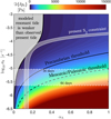Fig. 5

Parametric study of the tidal response. Plotted is a contoured surface of the amplitude of the imaginary part of the positive semidiurnal pressure anomaly at the Lamb resonance, over a grid of values of our free parameters σ₀ and α_A. The solid black isoline marks the level curve of Im{δp_s} = 880 Pa, and defines from below a region in (α_A, σ₀)-space where the thermotidal response is sufficient to cancel the gravitational counterpart in the Precambrian. Analogously, the dashed isoline defines the threshold needed in the late Paleozoic/early Meso-zoic, 350−250 Ma. The horizontal shaded area corresponds to typical values of the radiative cooling rate as described in the main text. The other shaded area defines the region of parameter space that yields the presently observed semi-diurnal tidal bulge. The gray area on the left covers the parametric region where the resonance features a lower pressure amplitude than the present.

4.2 The spectral position of the Lamb resonance

The spectral position of the Lamb resonance, or equivalently, the geological time of its occurrence, is identified in the analytical model via the denominator highlighted in Eq. (22). The latter is a function of σ and is dependent on the planetary radius, gravitational acceleration, eigenvalue of the fundamental Hough mode, the radiative frequency, and the equilibrium surface temperature at the surface T_s, and is independent of σ_bl. Thus for the Earth, the resonance position is merely dependent on the equilibrium temperature at the surface and the radiative cooling frequency.

In Fig. 6, we plot the dependence of the spectral position of the resonance, in terms of LOD, on T_s. The apparent single solid curve of the dry adiabatic profile is actually a bundle of curves with different values of σ₀, but the effect of the latter is unnoticeable (if one varies σ₀ by two orders of magnitude, the resonant rotational period varies by few minutes). As such, the resonant frequency is predominantly controlled by T_s, which allows us to take the adiabatic limit of Eq. (22), and straightforwardly derive the tidal frequency that minimizes the denominator. In terms of the rotational period, the position of the resonance then reads:

${LOD}_{res} = \frac{4 π R_{p}}{\sqrt{ℛ_{s} Λ_{n} T_{s}} + 2 R_{p} n_{⋆}} .$ ${\rm{LO}}{{\rm{D}}_{{\rm{res}}}} = {{4\pi {R_{\rm{p}}}} \over {\sqrt {{{\cal R}_{\rm{s}}}{{\rm{\Lambda }}_n}{T_{\rm{s}}}} + 2{R_{\rm{p}}}{n_ \star }}}.$ (24)

In Appendix I, we compute the tidal solution in the limit of a moist adiabatic profile by modifying the thermodynamic equation to allow for the effect of humidity. There we show that the same expression of the resonant period holds in the moist adiabatic limit. In Appendix M, we derive the analogous expression in the limit of an isothermal atmospheric profile, and we show that the resonant period is reduced by almost one hour compared to that in the adiabatic limit when a fixed enthalpy is considered for an air column in the two limits. For all profiles, nonetheless, the resonant rotational period scales as the inverse square root of the surface equilibrium temperature. However, the evolution of the latter for the early Earth is widely debated. For instance, marine oxygen isotopes have been interpreted to indicate Archean ocean temperatures around 60–80° C (e.g., Knauth 2005; Robert & Chaussidon 2006). This interpretation is in contrast with geochemical analysis using phosphates (e.g., Blake et al. 2010), geological evidence of Archean glacial deposits (e.g., de Wit & Furnes 2016), geological carbon cycle models (e.g., Sleep & Zahnle 2001; Krissansen-Totton et al. 2018), numerical results of 3D GCMs (e.g., Charnay et al. 2017), and the fact that solar luminosity was 10–25% lower during the Precambrian (e.g., Charnay et al. 2020), altogether predicting a temperate climate and moderate temperatures throughout the Earth’s history.

We highlight with the gray shading on top of the curves modeled mean surface temperature variations adopted from Krissansen-Totton et al. (2018). As the latter temperature evolution is established in the time domain, we use the LOD evolution in Farhat et al. (2022) to map from time-dependence to LOD-dependence, and we further identify the corresponding geological eras of the LOD evolution with the color shadings. Given the present-day equilibrium surface temperature, the resonance occurs at LOD = 22.8 h. This value is in agreement with the 11.38 ± 0.16 h semi-diurnal period obtained by analyzing the spectrum of normal modes using pressure data on global scales (see Table 1 of Sakazaki & Hamilton 2020, first symmetric gravity mode of wavenumber k = −2). The resonant rotational period assuming an isothermal profile of the atmosphere is roughly one hour less than that in the neutrally stratified limit, placing it closer to 21.3 h estimate of Zahnle & Walker (1987) and Bartlett & Stevenson (2016). We emphasize here, however, that the resonant period does not exactly mark the period at which the thermotidal torque is maximum. The latter occurs at the peaks surrounding the resonance (see Figs. 2 and H.1), the difference between the two being dependent on the radiative cooling frequency.

Taking the LOD evolution model of Farhat et al. (2022) at face value, the temperature variations predicted in Krissansen-Totton et al. (2018) locate the resonance encounter in the early Mesozoic (or late Paleozoic if one considers wider temperature variations), and not in the Precambrian. In fact, for the resonance to be encountered in the Precambrian, even in the latest eras of it, the resonant period should move to less than ~21 h, but this requires an increase in the equilibrium temperature of at least 55°C, which is inconsistent with the studies mentioned above. Such an increase in temperature would also increase σ₀ by almost 19% (as we discuss in the previous section, $σ_{0} \propto T_{0}^{3}$ ${\sigma _0} \propto T_0^3$ ; see also Appendix L), reducing the radiative cooling timescale and prompting more efficient damping of the tidal amplitude at the resonance. Moreover, such an increase in temperature would accompany increased greenhouse effects in the past, which in turn would increase the atmospheric absorption and thermotidal heating in the infrared. The latter would then place the Earth’s atmosphere in the regime of asynchronous thermotidal heating studied in Sect. 3.2, whereby the accelerative peak of the torque is further attenuated.

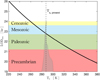Fig. 6

Dependence of the resonant rotational period on the mean surface temperature. By virtue of Eq. (24), the LOD at which the Lamb resonance occurs scales as the inverse square root of the mean surface temperature (solid curve). In Appendix I, we show that the same dependence holds if one considers a moist adiabatic profile. The shaded area of temperature variations highlights 95% confidence intervals for the past temperature evolution according to the carbon cycle model of Krissansen-Totton et al. (2018). The identified geological eras correspond to the LOD evolution model of Farhat et al. (2022). The overlap between the modeled temperature evolution and the black curve places the resonance occurrence in the late Paleozoic/early Mesozoic.

5 Summary and outlook

We were drawn to the problem of atmospheric thermal tides by the hypothesized scenario of a constant length of day on Earth during the Precambrian. Our motivation in investigating the scenario lies in its significant implications on paleoclimatic evolution, and the evident mismatch between LOD geological proxies and the predicted LOD evolution if this rotational equilibrium is surmised. The scenario hinges on the occurrence of a Lamb resonance in the atmosphere whereby an amplified thermotidal torque would cancel the opposing torque generated by solid and oceanic gravitational tides. Naturally, the atmospheric tidal torque is that of two flavors: it can either pump or deplete the rotational angular momentum budget of the planet, depending on the orientation of the generated tidal bulge.

With this rotational equilibrium scenario in mind, we have developed a novel analytical model that describes the tidal response of thermally forced atmospheres on rocky planets. The model derivation is based on the secure ground of the first principles of linear atmospheric dynamics, studied under classical approximations that are commonly drawn in earlier analytical works and in more recent numerical frameworks. The distinct feature that we imposed in this model is that of neutral atmospheric stratification, which presents a more realistic description of the Earth’s troposphere than the isothermal profile imposed in earlier analytical studies. In this limit, we derive from the model a closed-form solution of the tidal torque that can be efficiently used to study the evolution of planetary rotational dynamics. We accommodate into the model dissipative thermal radiation via linear Newtonian cooling, and turbulent and diffusive processes related to thermal inertia budgets in the boundary layer and the ground. As such, the model can be used to study a planetary thermotidal response when heated either by direct synchronous absorption of the incident stellar flux, or by a delayed infrared radiation from the ground.

We probed the spectral behavior of the tidal torque using this developed model in the two aforementioned limits. In the limit of longwave heating flux, the inherently delayed thermal response in the planetary boundary layer maneuvers the tidal bulge in such a way that, for typical values of thermal inertia in the ground and atmosphere, the accelerating effect of the tidal torque at the Lamb resonance is attenuated, and possibly annihilated. In the case of the Earth, where we apply the opposite limit of shortwave thermotidal heating and ignore the attenuating effect of asynchronous forcing, while the encounter of the resonance in the atmosphere is guaranteed, the epoch of its occurrence and the tidal amplitude it generates are uncertain. As such, we attempted a cautious incursion on constraining them and learned that:

Assuming that temperate climatic conditions have prevailed over the Earth’s history, the resonance is likely to have occurred in the late Paleozoic/early Mesozoic, and not in the Precambrian. Unlike the Precambrian, this era is characterized by an amplified decelerating luni-solar gravitational torque;
For judiciously constrained estimates of our atmospheric model parameters, the resonance does not amplify the accelerating thermotidal torque to a level comparable in magnitude to the gravitational counterpart in the said era.

It is important to note that these model predictions presume that thermotidal heating in the Earth has always been dominated by the shortwave. Compositional variations however, namely those associated with increased greenhouse contributions in the past would amplify the asynchronous thermotidal forcing in the longwave. The latter in turn, as we show in this work, further attenuates the accelerating flavor of the resonant torque. Exploring this end is certainly worthy of future efforts, but with the present indications at hand, we conclude that the occurrence of the rotational equilibrium is contingent upon a drastic increase in the Earth’s surface temperature (≥ 55°C), a long enough radiative cooling timescale (≥40 days), an increase in the shortwave flux opacity of the atmosphere, and that infrared thermotidal heating remained negligible in the past. We cannot completely preclude these requirements when considered separately, especially given the uncertainty in reconstructing the Earth’s temperature evolution in the Proterozoic. However, a warmer paleoclimate goes hand in hand with a shorter radiative cooling timescale, along with increased greenhouse gases that amplify the asynchronous thermotidal forcing. Both effects damp the accelerating flavor of the thermotidal torque. Put together, these indications suggest that the occurrence of the rotational equilibrium for the Earth is unlikely. To this end, future GCM simulations that properly model the Precambrian Earth to provide stringent constraints on our analytical predictions of the resonant amplification are certainly welcome.

Ultimately though, even if the locking into the resonance did not occur, the effect of the thermotidal torque at the resonance remains a robust and significant feature, and it should be accommodated in future modeling attempts of the Earth’s rotational evolution. Our model sets the table for efficiently studying such a complex interplay between several tidal players, both for the Earth and duly for its analogs. Interestingly, the question of the climatic response to the Lamb resonance, or similarly to oceanic tidal resonances, where abrupt and significant astronomical variations occur, largely remains an unexplored territory, perhaps requiring an armada of rigorous GCM simulations. This only leaves us with anticipated pleasure in weaving yet another thread in the rich tidal history of the Earth. Furthermore, we anticipate that the growing abundance of geological proxies, especially robust inferences associated with cyclostratigraphy, may help detect the whereabouts of these resonances and provide further constraints to our modeling efforts.

Acknowledgements

The authors are thankful to the referee, Dorian Abbot, for insightful comments which helped improve the manuscript considerably. M.F. expresses his gratitude to Kevin Heng for his hospitality at the LMU Munich Observatory where part of this work was completed. This work has been supported by the French Agence Nationale de la Recherche (AstroMeso ANR-19-CE31-0002-01) and by the European Research Council (ERC) under the European Union’s Horizon 2020 research and innovation program (Advanced Grant AstroGeo-885250). This work was granted access to the HPC resources of MesoPSL financed by the Region Île-de-France and the project Equip@Meso (reference ANR-10-EQPX-29-01) of the programme Investissements d’Avenir supervised by the Agence Nationale pour la Recherche.

Appendix A The dimensionless governing equations of atmospheric tidal dynamics

Using the same definition of atmospheric variables as in the main text, we develop here the dimensionless governing system of equations describing tidal dynamics, which shall be used to recover the wave equation (2). We start with the classical primitive equations describing the atmospheric tidal response under the thin shell approximation (e.g., Siebert 1961; Chapman & Lindzen 1970), and we augment the heat transfer equation by the additional radiative term J_rad described in the main text. These equations read:

$\partial_{t} V_{θ} - 2 Ω \cos θ V_{φ} = - \frac{1}{R_{p}} \partial_{θ} (\frac{δ p}{ρ_{0}} - U),$ ${\partial _t}{V_\theta } - 2{\rm{\Omega }}\cos \theta {V_\varphi } = - {1 \over {{R_{\rm{p}}}}}{\partial _\theta }\left( {{{\delta p} \over {{\rho _0}}} - U} \right),$ (A.1) $\partial_{t} V_{φ} + 2 Ω \cos θ V_{θ} = - \frac{1}{R_{p} \sin θ} \partial_{φ} (\frac{δ p}{ρ_{0}} - U),$ ${\partial _t}{V_\varphi } + 2{\rm{\Omega }}\cos \theta {V_\theta } = - {1 \over {{R_{\rm{p}}}\sin \theta }}{\partial _\varphi }\left( {{{\delta p} \over {{\rho _0}}} - U} \right),$ (A.2) $0 = - \partial_{z} δ p - g δ ρ + ρ_{0} \partial_{z} U,$ $0 = - {\partial _z}\delta p - g\delta \rho + {\rho _0}{\partial _z}U,$ (A.3) $\frac{D ρ}{D t} = - ρ_{0} χ,$ ${{D\rho } \over {Dt}} = - {\rho _0}\chi ,$ (A.4) $\frac{1}{Γ_{1}} \frac{D p}{D t} - g H \frac{D ρ}{D t} = κ ρ_{0} J - ρ_{0} ℛ_{s} σ_{0} δ T,$ ${1 \over {{{\rm{\Gamma }}_1}}}{{Dp} \over {Dt}} - gH{{D\rho } \over {Dt}} = \kappa {\rho _0}J - {\rho _0}{{\cal R}_{\rm{s}}}{\sigma _0}\delta T,$ (A.5) $χ - \partial_{z} V_{r} = \nabla_{h} \cdot V,$ $\chi - {\partial _z}{V_r} = {\nabla _{\rm{h}}} \cdot {\bf{V}},$ (A.6) $\frac{δ p}{p_{0}} = \frac{δ ρ}{ρ_{0}} + \frac{δ T}{T_{0}} .$ ${{\delta p} \over {{p_0}}} = {{\delta \rho } \over {{\rho _0}}} + {{\delta T} \over {{T_0}}}.$ (A.7)

This system describes atmospheric momentum conservation (Eqs. A.1 - A.3), mass conservation (Eq. A.4), heat transfer with Newtonian cooling (Eq. A.5), and the ideal gas law (Eq. A.7). Furthermore, we have adopted the traditional approximation (e.g., Unno et al. 1979), where we ignore the Coriolis coupling term between the vertical and horizontal parts of the momentum equations, thus allowing for the analytical treatment of the system. For the vertical momentum equation (A.3), the traditional approximation amounts to imposing the hydrostatic equilibrium for the tidal perturbation in addition to the background profiles, which are in turn averaged over the sphere. The hydrostatic approximation would allow us later to define the tidal torque as a function of the pressure anomaly at the surface.

In this system, the material (read Lagrangian) time derivative $\frac{D}{D t}$ ${D \over {Dt}}$ of any variable y is defined as

$\frac{D y}{D t} = \partial_{t} y + V_{r} \frac{d y_{0}}{d z},$ ${{Dy} \over {Dt}} = {\partial _t}y + {V_r}{{d{y_0}} \over {dz}},$ (A.8)

and we denote by χ the divergence of the velocity vector field V, and by the notation ∇_h · V its horizontal divergence such that

$\nabla_{h} \cdot V = \frac{1}{R_{p} \sin θ} [\partial_{θ} (\sin θ V_{θ}) + \partial_{φ} V_{φ}] .$ ${\nabla _{\rm{h}}} \cdot {\bf{V}} = {1 \over {{R_{\rm{p}}}\sin \theta }}\left[ {{\partial _\theta }\left( {\sin \theta {V_\theta }} \right) + {\partial _\varphi }{V_\varphi }} \right].$ (A.9)

We also introduce the calculation variable

$G = - \frac{1}{Γ_{1} p_{0}} \frac{D p}{D t} .$ $G = - {1 \over {{{\rm{\Gamma }}_1}{p_0}}}{{Dp} \over {Dt}}.$ (A.10)

It is noteworthy here, as we impose neutral stratification on the atmosphere later in the model (Section 3.1), that one can argue that the gôp term in Eq.(A.3) is supposed to vanish since it is often referred to as the buoyancy term. However, this is not exactly the case since internal gravity waves are not the only source of density fluctuations. In fact, density fluctuations can also result from the planetary-scale compressibility waves, read Lamb modes. As such, the atmosphere can be at the same time neutrally stratified and still feature strong density variations across the horizontal direction. With this subtlety clarified, the tidal perturbations are then expanded in Fourier series of time and longitude, such that the tidal excitation frequency is denoted by σ. We introduce the reference velocity υ₀, and we non-dimensionalize all the variables; namely:

$\begin{array}{l} d z = H d x, t = σ^{- 1} \tilde{t}, V = v_{0} \tilde{V}, δ p = p_{0} \tilde{δ} p, \\ δ ρ = ρ_{0} \tilde{δ} ρ, δ T = T_{0} \tilde{δ} T, U = v_{0}^{2} \tilde{U}, G = \frac{σ}{Γ_{1}} \tilde{G}, \\ \nabla_{h \cdot} = R_{p}^{- 1} \tilde{\nabla} \cdot, \nabla_{h} = R_{p}^{- 1} \tilde{\nabla}, J = \frac{σ g H}{κ} \tilde{J}, \end{array}$ $\matrix{ {dz = Hdx,\quad t = {\sigma ^{ - 1}}\tilde t,\quad {\bf{V}} = {v_0}{\bf{\tilde V}},\quad \delta p = {p_0}\widetilde \delta p,} \hfill \cr {\delta \rho = {\rho _0}\widetilde \delta \rho ,\quad \delta T = {T_0}\widetilde \delta T,\quad U = v_0^2\tilde U,\quad G = {\sigma \over {{{\rm{\Gamma }}_1}}}\tilde G,} \hfill \cr {{\nabla _{\rm{h}}} = R_{\rm{p}}^{ - 1}\tilde \nabla \cdot ,\quad {\nabla _{\rm{h}}} = R_{\rm{p}}^{ - 1}\tilde \nabla ,\quad J = {{\sigma gH} \over \kappa }\tilde J,} \hfill \cr }$ (A.11)

Under these definitions, the material derivative now reads

$\frac{D y}{D t} = σ y_{0} [\partial_{\tilde{t}} \tilde{δ} y + \frac{v_{0}}{σ H} \frac{d \ln y_{0}}{d x} {\tilde{V}}_{r}],$ ${{Dy} \over {Dt}} = \sigma {y_0}\left[ {{\partial _{\tilde t}}\tilde \delta y + {{{v_0}} \over {\sigma H}}{{d\ln {y_0}} \over {dx}}{{\tilde V}_r}} \right]{\rm{,}}$ (A.12)

and the calculation variable $\tilde{G}$ ${\tilde G}$ becomes

$\partial_{\tilde{t}} \tilde{δ} p + \frac{υ_{0}}{σ H} \frac{d \ln p_{0}}{d x} {\tilde{V}}_{r} = - \tilde{G} .$ ${\partial _{\tilde t}}\widetilde \delta p + {{{\upsilon _0}} \over {\sigma H}}{{d\ln {p_0}} \over {dx}}{\tilde V_r} = - \tilde G.$ (A.13)

We next set υ₀ = σR_p and introduce the ratios of length scale η = R_p /H, and frequency α = σ/σ₀. Allowing for these changes of variables in the governing system of equations, one directly obtains a dimensionless system in the form:

$\partial_{\tilde{t}} {\tilde{V}}_{θ} - v \cos θ {\tilde{V}}_{φ} = - \partial_{θ} (\frac{g H}{υ_{0}^{2}} \tilde{δ} p - \tilde{U}),$ ${\partial _{\tilde t}}{\tilde V_\theta } - v\cos \theta {\tilde V_\varphi } = - {\partial _\theta }\left( {{{gH} \over {\upsilon _0^2}}\widetilde \delta p - \tilde U} \right),$ (A.14) $\partial_{\tilde{t}} {\tilde{V}}_{φ} + v \cos θ {\tilde{V}}_{θ} = - \frac{1}{\sin θ} \partial_{φ} (\frac{g H}{υ_{0}^{2}} \tilde{δ} p - \tilde{U}),$ ${\partial _{\tilde t}}{\tilde V_\varphi } + v\cos \theta {\tilde V_\theta } = - {1 \over {\sin \theta }}{\partial _\varphi }\left( {{{gH} \over {\upsilon _0^2}}\widetilde \delta p - \tilde U} \right),$ (A.15) $(\partial_{x} - 1) \tilde{δ} p = - \tilde{δ} ρ + \frac{υ_{0}^{2}}{g H} \partial_{x} \tilde{U},$ $\left( {{\partial _x} - 1} \right)\widetilde \delta p = - \widetilde \delta \rho + {{\upsilon _0^2} \over {gH}}{\partial _x}\tilde U,$ (A.16) $\partial_{\tilde{t}} \tilde{δ} + \tilde{\nabla} \cdot \tilde{V} = - η (\partial_{x} + \frac{d \ln ρ_{0}}{d x}) {\tilde{V}}_{r},$ ${\partial _{\tilde t}}\tilde \delta + \tilde \nabla \cdot {\bf{\tilde V}} = - \eta \left( {{\partial _x} + {{d\ln {\rho _0}} \over {dx}}} \right){\tilde V_r},$ (A.17) $\frac{\tilde{G}}{Γ_{1}} + \partial_{\tilde{t}} \tilde{δ} ρ + η \frac{d \ln ρ_{0}}{d x} {\tilde{V}}_{r} = - \tilde{J} + \frac{δ \tilde{T}}{α},$ ${{\tilde G} \over {{{\rm{\Gamma }}_1}}} + {\partial _{\tilde t}}\widetilde \delta \rho + \eta {{d\ln {\rho _0}} \over {dx}}{\tilde V_r} = - \tilde J + {{\delta \tilde T} \over \alpha },$ (A.18) $\tilde{δ} p = \tilde{δ} ρ + \tilde{δ} T .$ $\widetilde \delta p = \widetilde \delta \rho + \widetilde \delta T.$ (A.19)

Due to the periodic nature of the tidal forcing, the tidal response is Fourier-decomposed in time and longitude, allowing us to write all the physically varying quantities in the form

$f (x, θ, φ, \tilde{t}) = Re {\underset{m}{\sum^{}} f^{m, v} (x, θ) e^{i (\tilde{t} + m φ)}},$ $f\left( {x,\theta ,\varphi ,\tilde t} \right) = {\mathop{\rm Re}\nolimits} \left\{ {\mathop {\mathop \sum \nolimits^ }\limits_m {f^{m,v}}\left( {x,\theta } \right){e^{i(\tilde t + m\varphi )}}} \right\},$ (A.20)

where m is the longitudinal degree. Furthermore, due to the traditional approximation, the decoupling of the vertical and horizontal structures of tidal dynamics allows the expansion of the Fourier coefficients of Eq. (A.20) into series of Hough functions (Hough 1898) describing the horizontal tidal flow; namely:

$f^{m, v} (x, θ) = \underset{n}{\sum^{}} f_{n}^{m, v} (x) Θ_{n}^{m, v} (θ) .$ ${f^{m,v}}(x,\theta ) = \mathop {\mathop \sum \nolimits^ }\limits_n f_n^{m,v}(x){\rm{\Theta }}_n^{m,v}(\theta ).$ (A.21)

Unless stated otherwise, we denote throughout the paper the coefficients $f_{n}^{m, v}$ $f_n^{m,v}$ by f_n for simplicity. As such, the Laplace tidal equation given in the main text by Eq. (1) is rewritten as:

$ℒ Θ_{n} = - Λ_{n} Θ_{n},$ ${\cal L}{{\rm{\Theta }}_n} = - {{\rm{\Lambda }}_n}{{\rm{\Theta }}_n},$ (A.22)

where the operator ℒ is defined as

$\begin{array}{l} ℒ = \frac{1}{\sin θ} \frac{d}{d θ} (\frac{\sin θ}{1 - v^{2} \cos^{2} θ} \frac{d}{d θ}) \\ - \frac{1}{1 - v^{2} \cos^{2} θ} (m v \frac{1 + v^{2} \cos^{2} θ}{1 - v^{2} \cos^{2} θ} + \frac{m^{2}}{\sin^{2} θ}) . \end{array}$ $\matrix{ {{\cal L} = {1 \over {\sin \theta }}{d \over {d\theta }}\left( {{{\sin \theta } \over {1 - {v^2}{{\cos }^2}\theta }}{d \over {d\theta }}} \right)} \hfill \cr {\,\,\,\,\, - {1 \over {1 - {v^2}{{\cos }^2}\theta }}\left( {mv{{1 + {v^2}{{\cos }^2}\theta } \over {1 - {v^2}{{\cos }^2}\theta }} + {{{m^2}} \over {{{\sin }^2}\theta }}} \right).} \hfill \cr }$ (A.23)

Appendix B Retrieving the wave equation of vertical dynamics

The governing system of dimensionless equations (A.14-A.19) decouples into equations describing the horizontal structure (A.14-A.15), and those describing the vertical structure. In the Fourier domain, the latter equations read:

$i \tilde{δ} p_{n} - η {\tilde{V}}_{r; n} = - {\tilde{G}}_{n},$ $i\widetilde \delta {p_n} - \eta {\tilde V_{r;n}} = - {\tilde G_n},$ (B.1) $(\partial_{x} - 1) \tilde{δ} p_{n} = - \tilde{δ} ρ_{n} + \frac{v_{0}^{2}}{g H} \partial_{x} {\tilde{U}}_{n},$ $\left( {{\partial _x} - 1} \right)\widetilde \delta {p_n} = - \tilde \delta {\rho _n} + {{v_0^2} \over {gH}}{\partial _x}{\tilde U_n},$ (B.2) $\tilde{δ} ρ_{n} - i η (\partial_{x} + \frac{d \ln ρ_{0}}{d x}) {\tilde{V}}_{r; n} = - ℒ (\frac{g H}{v_{0}^{2}} \tilde{δ} p_{n} - {\tilde{U}}_{n}),$ $\widetilde \delta {\rho _n} - i\eta \left( {{\partial _x} + {{d\ln {\rho _0}} \over {dx}}} \right){\tilde V_{r;n}} = - {\cal L}\left( {{{gH} \over {v_0^2}}\widetilde \delta {p_n} - {{\tilde U}_n}} \right){\rm{,}}$ (B.3) $\frac{{\tilde{G}}_{n}}{Γ_{1}} + i \tilde{δ} ρ_{n} + η \frac{d \ln ρ_{0}}{d x} {\tilde{V}}_{r; n} = - {\tilde{J}}_{n} + \frac{δ T_{n}}{α},$ ${{{{\tilde G}_n}} \over {{{\rm{\Gamma }}_1}}} + i\widetilde \delta {\rho _n} + \eta {{d\ln {\rho _0}} \over {dx}}{\tilde V_{r;n}} = - {\tilde J_n} + {{\delta {T_n}} \over \alpha },$ (B.4) $\tilde{δ} p_{n} = \tilde{δ} ρ_{n} + \tilde{δ} T_{n} .$ $\widetilde \delta {p_n} = \widetilde \delta {\rho _n} + \widetilde \delta {T_n}.$ (B.5)

To recover the wave equation (2) from this system, we aim to reduce this system to a single second order partial differential equation in the calculation variable ${\tilde{G}}_{n}$ ${{\tilde G}_n}$ . First, we combine Eq. (B.1) with the heat transfer equation (B.4) to eliminate the vertical component of velocity, ${\tilde{V}}_{r; n}$ ${{\tilde V}_{r;n}}$ . Then we use the ideal gas law (B.5) to replace $\tilde{δ} T_{n}$ $\tilde \delta {T_n}$ by $\tilde{δ} p_{n}$ $\tilde \delta {p_n}$ and $\tilde{δ} ρ_{n}$ $\tilde \delta {\rho _n}$ in the resulting equation. It follows that

$\tilde{δ} p_{n} (1 + \frac{d \ln H}{d x} - \frac{i}{α}) - \tilde{δ} ρ_{n} (1 - \frac{i}{α}) = \frac{i N_{B}^{2} H}{g} {\tilde{G}}_{n} - i {\tilde{J}}_{n} .$ $\widetilde \delta {p_n}\left( {1 + {{d\ln H} \over {dx}} - {i \over \alpha }} \right) - \widetilde \delta {\rho _n}\left( {1 - {i \over \alpha }} \right) = {{iN_{\rm{B}}^2H} \over g}{\tilde G_n} - i{\tilde J_n}{\rm{.}}$ (B.6)

Next, we use the hydrostatic equilibrium condition (B.2) to express $\tilde{δ} ρ_{n}$ $\tilde \delta {\rho _n}$ in terms of $\tilde{δ} p_{n}$ $\tilde \delta {p_n}$ and Ũ_n in the above equation to obtain

$\partial_{x} \tilde{δ} p_{n} = i \frac{α H N_{B}^{2}}{g (α - i)} {\tilde{G}}_{n} - \frac{α}{α - i} \frac{d \ln H}{d x} \tilde{δ} p_{n} - \frac{i α}{α - i} {\tilde{J}}_{n} + \frac{υ_{0}^{2}}{g H} \partial_{x} {\tilde{U}}_{n} .$ ${\partial _x}\widetilde \delta {p_n} = i{{\alpha HN_{\rm{B}}^2} \over {g(\alpha - i)}}{\tilde G_n} - {\alpha \over {\alpha - i}}{{d\ln H} \over {dx}}\widetilde \delta {p_n} - {{i\alpha } \over {\alpha - i}}{\tilde J_n} + {{\upsilon _0^2} \over {gH}}{\partial _x}{\tilde U_n}.$ (B.7)

Now our aim is to obtain another first order equation in the calculation variable ${\tilde{G}}_{n}$ ${{\tilde G}_n}$ . We start with the hydrostatic equilibrium condition (B.2), and we substitute $\tilde{δ} p_{n}$ $\tilde \delta {p_n}$ by its expression (B.1). Then we use the continuity equation (B.3) to express $\tilde{δ} ρ_{n}$ $\tilde \delta {\rho _n}$ as a function of ${\tilde{V}}_{r; n}$ ${{\tilde V}_{r;n}}$ and $\tilde{δ} p_{n}$ $\tilde \delta {p_n}$ , and we finally eliminate ${\tilde{V}}_{r; n}$ ${{\tilde V}_{r;n}}$ using equation (B.1) to obtain

$\partial_{x} {\tilde{G}}_{n} = {\tilde{G}}_{n} - i \frac{g H}{v_{0}^{2}} ℒ {\tilde{δ}}_{n} + i (ℒ - \frac{υ_{0}^{2}}{g H} \partial_{x}) {\tilde{U}}_{n} .$ ${\partial _x}{\tilde G_n} = {\tilde G_n} - i{{gH} \over {v_0^2}}{\cal L}{\tilde \delta _n} + i\left( {{\cal L} - {{\upsilon _0^2} \over {gH}}{\partial _x}} \right){\tilde U_n}.$ (B.8)

We thus have two first order partial differential equations (B.7 - B.8) of the form

$\partial_{x} {\tilde{G}}_{n} = A_{1} {\tilde{G}}_{n} + B_{1} \tilde{δ} p_{n} + C_{1},$ ${\partial _x}{\tilde G_n} = {A_1}{\tilde G_n} + {B_1}\widetilde \delta {p_n} + {C_1},$ (B.9) $\partial_{x} \tilde{δ} p p_{n} = A_{2} {\tilde{G}}_{n} + B_{2} \tilde{δ} p_{n} + C_{2} .$ ${\partial _x}\widetilde \delta p{p_n} = {A_2}{\tilde G_n} + {B_2}\widetilde \delta {p_n} + {C_2}.$ (B.10)

Taking the derivative of Eq.(B.9), it is straightforward to obtain a second order equation of the form:

$[\partial_{x}^{2} + A \partial_{x} + B] {\tilde{G}}_{n} = C_{n},$ $\left[ {\partial _x^2 + A{\partial _x} + B} \right]{\tilde G_n} = {C_n},$ (B.11)

where

$A (x) = - 1 + \frac{i}{α - i} \frac{d \ln H}{d x},$ $A(x) = - 1 + {i \over {\alpha - i}}{{d\ln H} \over {dx}},$ (B.12) $B (x) = - \frac{α}{α - i} [\frac{i}{α} \frac{d \ln H}{d x} + \frac{H^{2} N_{B}^{2}}{v_{0}^{2}} ℒ],$ $B(x) = - {\alpha \over {\alpha - i}}\left[ {{i \over \alpha }{{d\ln H} \over {dx}} + {{{H^2}N_{\rm{B}}^2} \over {v_0^2}}{\cal L}} \right]{\rm{,}}$ (B.13) $C_{n} (x) = - \frac{g H α}{v_{0}^{2} (α - i)} ℒ {\tilde{J}}_{n} - [i \frac{d}{d x} (\frac{v_{0}^{2}}{g H} \frac{d}{d x})$ ${C_n}(x) = - {{gH\alpha } \over {v_0^2(\alpha - i)}}{\cal L}{\tilde J_n} - \left[ {i{d \over {dx}}\left( {{{v_0^2} \over {gH}}{d \over {dx}}} \right)} \right.$ (B.14) $+ \frac{1}{α - i} \frac{d \ln H}{d x} (ℒ - \frac{υ_{0}^{2}}{g H} \frac{d}{d x})] {\tilde{U}}_{n} .$ $\left. { + {1 \over {\alpha - i}}{{d\ln H} \over {dx}}\left( {{\cal L} - {{\upsilon _0^2} \over {gH}}{d \over {dx}}} \right)} \right]{\tilde U_n}.$ (B.15)

Next, we implement a change of variable of the form ${\tilde{G}}_{n} (x) = Φ (x) Ψ_{n} (x)$ ${{\tilde G}_n}(x) = {\rm{\Phi }}(x){{\rm{\Psi }}_n}(x)$ to write Eq. (B.11) in the standard form of wave equations. We find that the first order term in Eq. (B.11) cancels when

$2 \frac{d Φ (x)}{d x} + A (x) Φ (x) = 0,$ $2{{d{\rm{\Phi }}(x)} \over {dx}} + A(x){\rm{\Phi }}(x) = 0,$ (B.16)

which is satisfied by

$Φ (x) = \exp (- \frac{1}{2} {\int^{}}_{0}^{x} A (x^{'}) d x^{'}) .$ ${\rm{\Phi }}(x) = \exp \left( { - {1 \over 2}\mathop \smallint \nolimits^ _0^xA\left( {x'} \right)dx'} \right).$ (B.17)

This gives us the form of Φ(x) defined in Eq. (5), and consequently the wave equation (2), with a vertical wavenumber $\hat{k}$ ${\hat k}$ defined as

$\begin{array}{l} {\hat{k}}_{n}^{2} = - \frac{1}{4} (A^{2} + 2 \frac{d A}{d x} - 4 B) \\ = - \frac{1}{4} {{(1 - \frac{i}{α - i} \frac{d \ln H}{d x})}^{2} + 2 \frac{d}{d x} (\frac{i}{α - i} \frac{d \ln H}{d x}) \\ - \frac{4 α}{α - i} [\frac{g H N_{B}^{2} Λ_{n}}{v_{0}^{2}} - \frac{i}{α} \frac{d \ln H}{d x}]} . \end{array}$ $\matrix{ {\hat k_n^2 = - {1 \over 4}\left( {{A^2} + 2{{dA} \over {dx}} - 4B} \right)} \hfill \cr {\,\,\,\,\,\, = - {1 \over 4}\left\{ {{{\left( {1 - {i \over {\alpha - i}}{{d\ln H} \over {dx}}} \right)}^2} + 2{d \over {dx}}\left( {{i \over {\alpha - i}}{{d\ln H} \over {dx}}} \right)} \right.} \hfill \cr {\left. {\,\,\,\,\,\, - {{4\alpha } \over {\alpha - i}}\left[ {{{gHN_{\rm{B}}^2{{\rm{\Lambda }}_n}} \over {v_0^2}} - {i \over \alpha }{{d\ln H} \over {dx}}} \right]} \right\}.} \hfill \cr }$ (B.18)

With the definitions of the dimensionless control parameters given in Table 1, the wave number ${\hat{k}}_{n}$ ${{\hat k}_n}$ (Eq.B.18) and the forcing term (Eq.B.15) can be rewritten in the form given in the main text by Eqs. (3) and (6) respectively.

Appendix C Solutions of the vertical profiles of tidal variables

In this section we provide the solutions to the vertical profiles of the tidally varying scalar fields of pressure, density, and temperature, and the velocity vector field, given the solution of the wave equation Ψ(x)_n, or equivalently the variable ${\tilde{G}}_{n}$ ${{\tilde G}_n}$ .

First, the expression of pressure variations is readily obtained from Eq.(B.8), which for a given Hough mode and using the definition of β (Table 1) reads

$\tilde{δ} p_{n} = \frac{1}{i β Λ_{n}} (\frac{d {\tilde{G}}_{n}}{d x} - {\tilde{G}}_{n}) + \frac{1}{β} (1 + \frac{1}{β Λ_{n}} \frac{d}{d x}) {\tilde{U}}_{n} .$ $\widetilde \delta {p_n} = {1 \over {i\beta {{\rm{\Lambda }}_n}}}\left( {{{d{{\tilde G}_n}} \over {dx}} - {{\tilde G}_n}} \right) + {1 \over \beta }\left( {1 + {1 \over {\beta {{\rm{\Lambda }}_n}}}{d \over {dx}}} \right){\tilde U_n}.$ (C.1)

Given $\tilde{δ} p_{n} (x)$ $\tilde \delta {p_n}(x)$ , the horizontal component of the velocity field is straightforwardly obtained via (e.g., Eqs.(25-26) of Auclair-Desrotour et al. 2017b):

${\tilde{V}}_{θ; n} = \frac{\partial_{θ} + m v \cot θ}{1 - v^{2} \cos^{2} θ} (\frac{g H}{υ_{0}^{2}} \tilde{δ} p_{n} - {\tilde{U}}_{n}),$ ${\tilde V_{\theta ;n}} = {{{\partial _\theta } + mv\cot \theta } \over {1 - {v^2}{{\cos }^2}\theta }}\left( {{{gH} \over {\upsilon _0^2}}\widetilde \delta {p_n} - {{\tilde U}_n}} \right),$ (C.2)

${\tilde{V}}_{φ; n} = - \frac{v \cos θ \partial_{θ} + m \sin^{- 1} θ}{1 - v^{2} \cos^{2} θ} (\frac{g H}{v_{0}^{2}} \tilde{δ} p_{n} - {\tilde{U}}_{n}),$ ${\tilde V_{\varphi ;n}} = - {{v\cos \theta {\partial _\theta } + m{{\sin }^{ - 1}}\theta } \over {1 - {v^2}{{\cos }^2}\theta }}\left( {{{gH} \over {v_0^2}}\widetilde \delta {p_n} - {{\tilde U}_n}} \right),$ (C.3)

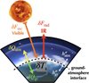Fig. D.1

Schematic of the bichromatic radiative and diffusive flux exchange mechanisms at the surface interface between the lower troposphere and the ground. The power balance between the fluxes in given by Eq. (D.1).

which gives

${\tilde{V}}_{θ; n} = \frac{1}{Λ_{n}} (\frac{d {\tilde{G}}_{n}}{d x} - {\tilde{G}}_{n} + i β^{- 1} \frac{d {\tilde{U}}_{n}}{d x}),$ ${\tilde V_{\theta ;n}} = {1 \over {{{\rm{\Lambda }}_n}}}\left( {{{d{{\tilde G}_n}} \over {dx}} - {{\tilde G}_n} + i{\beta ^{ - 1}}{{d{{\tilde U}_n}} \over {dx}}} \right),$ (C.4)

${\tilde{V}}_{φ; n} = \frac{i}{Λ_{n}} (\frac{d {\tilde{G}}_{n}}{d x} - {\tilde{G}}_{n} + i β^{- 1} \frac{d {\tilde{U}}_{n}}{d x}) .$ ${\tilde V_{\varphi ;n}} = {i \over {{{\rm{\Lambda }}_n}}}\left( {{{d{{\tilde G}_n}} \over {dx}} - {{\tilde G}_n} + i{\beta ^{ - 1}}{{d{{\tilde U}_n}} \over {dx}}} \right).$ (C.5)

The vertical component of the velocity is established from equation (B.1), replacing $\tilde{δ} p_{n}$ $\tilde \delta {p_n}$ by its solution (C.1):

${\tilde{V}}_{r; n} = \frac{1}{η β Λ_{n}} [\frac{d {\tilde{G}}_{n}}{d x} + (β Λ_{n} - 1) {\tilde{G}}_{n}] + \frac{i}{η β} (1 + \frac{1}{β Λ_{n}} \frac{d}{d x}) {\tilde{U}}_{n} .$ ${\tilde V_{r;n}} = {1 \over {\eta \beta {{\rm{\Lambda }}_n}}}\left[ {{{d{{\tilde G}_n}} \over {dx}} + \left( {\beta {{\rm{\Lambda }}_n} - 1} \right){{\tilde G}_n}} \right] + {i \over {\eta \beta }}\left( {1 + {1 \over {\beta {{\rm{\Lambda }}_n}}}{d \over {dx}}} \right){\tilde U_n}.$ (C.6)

Finally, the solution for the density perturbation is obtained by replacing the solution of $\tilde{δ} p_{n}$ $\tilde \delta {p_n}$ (C.1) in equation (B.6) to get:

$\begin{array}{l} \tilde{δ} ρ_{n} = \frac{1}{i β Λ_{n}} (1 + \frac{κ α (γ - 1)}{α - i}) [\frac{d {\tilde{G}}_{n}}{d x} + (\frac{α β γ κ Λ}{α - i + κ α (γ - 1)} - 1) {\tilde{G}}_{n}] \\ + \frac{i α {\tilde{J}}_{n}}{α - i} + \frac{1}{β} (1 + \frac{κ α (γ - 1)}{α - i}) (1 + \frac{1}{β Λ_{n}} \frac{d}{d x}) {\tilde{U}}_{n}, \end{array}$ $\matrix{ {\widetilde \delta {\rho _n} = {1 \over {i\beta {{\rm{\Lambda }}_n}}}\left( {1 + {{\kappa \alpha (\gamma - 1)} \over {\alpha - i}}} \right)\left[ {{{d{{\tilde G}_n}} \over {dx}} + \left( {{{\alpha \beta \gamma \kappa {\rm{\Lambda }}} \over {\alpha - i + \kappa \alpha (\gamma - 1)}} - 1} \right){{\tilde G}_n}} \right]} \hfill \cr {\,\,\,\,\,\,\,\,\,\, + {{i\alpha {{\tilde J}_n}} \over {\alpha - i}} + {1 \over \beta }\left( {1 + {{\kappa \alpha (\gamma - 1)} \over {\alpha - i}}} \right)\left( {1 + {1 \over {\beta {{\rm{\Lambda }}_n}}}{d \over {dx}}} \right){{\tilde U}_n},} \hfill \cr }$ (C.7)

and the vertical profile of temperature is then readily obtained by the ideal gas law (B.5).

Appendix D Thermal exchange mechanisms and the total propagating flux

We define here explicitly the thermal exchange mechanisms used to establish the thermal energy budget at the surface and to construct the thermal forcing profile given by Eq.(10) of Section 2.2.

As mentioned in the main text, the incident stellar flux, δF_inc generates a variation δT_s in the surface temperature T_s. We denote the proportionality by the complex transfer function $ℬ_{gr}^{σ}$ ${\cal B}_{{\rm{gr}}}^\sigma$ such that $δ T_{s} = ℬ_{gr}^{σ} δ F_{inc}$ $\delta {T_{\rm{s}}} = {\cal B}_{{\rm{gr}}}^\sigma \,\delta {F_{{\rm{inc}}}}$ . The variation δT_s induces radiative emission with magnitude δF_rad. A fraction of the incident power, δQ_gr, is then transmitted to the ground by thermal conduction, and another fraction, δQ_atm, is transmitted to the atmosphere through turbulent thermal diffusion (see Figure D.1).

Having isolated these thermal mechanisms, the total power balance of the thermal perturbation at the surface interface is expressed as⁸:

$δ F_{inc} - δ F_{rad} = δ Q_{gr} + δ Q_{atm} .$ $\delta {F_{{\rm{inc}}}} - \delta {F_{{\rm{rad}}}} = \delta {Q_{{\rm{gr}}}} + \delta {Q_{{\rm{atm}}}}.$ (D.1)

To define each of these terms explicitly, we start with the surface radiative emission term δF_rad, which can be obtained by differentiating the Stefan-Boltzmann law as a function of the surface temperature assuming that the planetary surface radiates as a black body. Namely we have

$δ F_{rad} = 4 σ_{SB} T_{s}^{3} δ T_{s},$ $\delta {F_{{\rm{rad}}}} = 4{\sigma _{{\rm{SB}}}}T_{\rm{s}}^3\delta {T_{\rm{s}}},$ (D.2)

with σ_SB = 5.670373 × 10⁻⁸ W m⁻² K⁻⁴ being the Stephan-Boltzmann constant (Tiesinga et al. 2021).

Next, the terms associated with heat diffusion at the boundary interface, δQ_gr and δQ_atm, are derived using the gradient flux theory (Garratt 1994):

$δ Q_{gr} (t) = {\frac{k_{gr}}{H} \frac{\partial δ T}{\partial x} |}_{x = 0^{-}},$ $\delta {Q_{{\rm{gr}}}}(t) = {\left. {{{{k_{{\rm{gr}}}}} \over H}{{\partial \delta T} \over {\partial x}}} \right|_{x = {0^ - }}},$ (D.3)

$δ Q_{atm} (t) = - {\frac{k_{atm}}{H} \frac{\partial δ T}{\partial x} |}_{x = 0^{+}} .$ $\delta {Q_{{\rm{atm}}}}(t) = - {\left. {{{{k_{{\rm{atm}}}}} \over H}{{\partial \delta T} \over {\partial x}}} \right|_{x = {0^ + }}}.$ (D.4)

Here, k_gr is the thermal conductivity of the ground, and k_atm is its atmospheric analog. We also denote by x = 0⁻ and x = 0⁺ the vicinity below and above the surface interface, respectively. Temperature variations near the surface can be traced by the heat transport equation, which in the frequency domain reads as (e.g., Chapman & Lindzen 1970)

$i σ δ T = \frac{K_{gr}}{H^{2}} \frac{\partial^{2} δ T}{\partial x^{2}} for x < 0,$ $i\sigma \delta T = {{{K_{{\rm{gr}}}}} \over {{H^2}}}{{{\partial ^2}\delta T} \over {\partial {x^2}}}\quad {\rm{for}}x < 0,$ (D.5)

$i σ δ T = \frac{K_{atm}}{H^{2}} \frac{\partial^{2} δ T}{\partial x^{2}} for x > 0,$ $i\sigma \delta T = {{{K_{{\rm{atm}}}}} \over {{H^2}}}{{{\partial ^2}\delta T} \over {\partial {x^2}}}\quad {\rm{for}}x > 0,$ (D.6)

with K_gr = k_gr/(ρ₀(0⁻)C_gr) and K_atm = k_atm/(ρ₀(0⁺)C_p) being the thermal diffusivities near the surface in the ground and the atmosphere respectively, C_gr and C_p being the respective thermal capacities per unit mass, while ρ₀(0⁻) and ρ₀(0⁺) are the densities in the vicinity of the surface interface. These equations have solutions of the form:

$δ T (x) = δ T_{s} \exp {(1 + i s) x / h_{gr}^{σ}}, for x \leq 0,$ $\delta T(x) = \delta {T_{\rm{s}}}\exp \left\{ {(1 + is)x/h_{{\rm{gr}}}^\sigma } \right\},\quad {\rm{for}}x \le 0,$ (D.7)

$δ T (x) = δ T_{s} \exp {- (1 + i s) x / h_{atm}^{σ}}, for x > 0.$ $\delta T(x) = \delta {T_{\rm{s}}}\exp \left\{ { - (1 + is)x/h_{{\rm{atm}}}^\sigma } \right\}{\rm{,}}\quad {\rm{for}}x > 0.{\rm{}}$ (D.8)

Here, we remind the reader that s = sgn(σ), and we denote by $h_{gr}^{σ}$ $h_{{\rm{gr}}}^\sigma$ and $h_{atm}^{σ}$ $h_{{\rm{atm}}}^\sigma$ the skin thicknesses of heat transport by thermal diffusion in the ground and the atmosphere defined as

$h_{gr}^{σ} = \frac{1}{H} \sqrt{\frac{2 K_{gr}}{| σ |}} and h_{atm}^{σ} = \frac{1}{H} \sqrt{\frac{2 K_{atm}}{| σ |}} .$ $h_{{\rm{gr}}}^\sigma = {1 \over H}\sqrt {{{2{K_{{\rm{gr}}}}} \over {|\sigma |}}} \quad {\rm{and}}\quad h_{{\rm{atm}}}^\sigma = {1 \over H}\sqrt {{{2{K_{{\rm{atm}}}}} \over {|\sigma |}}} .$ (D.9)

To obtain the explicit form of $ℬ_{gr}^{σ}$ ${\cal B}_{{\rm{gr}}}^\sigma$ , we first rewrite the power budget balance of Eq.(D.1) as

$δ F_{inc} - {\frac{k_{gr}}{H} \frac{\partial δ T}{\partial x} |}_{x = 0^{-}} = - {\frac{k_{atm}}{H} \frac{\partial δ T}{\partial x} |}_{x = 0^{+}} + 4 σ_{SB} T_{s}^{3} δ T_{s},$ $\delta {F_{{\rm{inc}}}} - {\left. {{{{k_{{\rm{gr}}}}} \over H}{{\partial \delta T} \over {\partial x}}} \right|_{x = {0^ - }}} = - {\left. {{{{k_{{\rm{atm}}}}} \over H}{{\partial \delta T} \over {\partial x}}} \right|_{x = {0^ + }}} + 4{\sigma _{{\rm{SB}}}}T_{\rm{s}}^3\delta {T_{\rm{s}}},$ (D.10)

and we substitute the solutions of δT(x) of Eq. (D.7) to obtain

$ℬ_{gr}^{σ} = {(4 σ_{SB} T_{s}^{3}) [1 + (1 + s i) \sqrt{τ_{bl} | σ |}]}^{- 1} .$ ${\cal B}_{{\rm{gr}}}^\sigma = {\left\{ {\left( {4{\sigma _{{\rm{SB}}}}T_{\rm{s}}^3} \right)\left[ {1 + (1 + si)\sqrt {{\tau _{{\rm{bl}}}}|\sigma |} } \right]} \right\}^{ - 1}}.$ (D.11)

Here we have defined the boundary layer timescale τ_bl as

$τ_{bl} = \frac{1}{2} {(\frac{I_{gr} + I_{atm}}{4 σ_{SB} T_{s}^{3}})}^{2},$ ${\tau _{{\rm{bl}}}} = {1 \over 2}{\left( {{{{I_{{\rm{gr}}}} + {I_{{\rm{atm}}}}} \over {4{\sigma _{{\rm{SB}}}}T_{\rm{s}}^3}}} \right)^2},$ (D.12)

where the functions I_gr and I_atm denote, respectively, the thermal inertias of the ground and the atmospheric surface layers, and are specifically given by:

$\begin{matrix} I_{gr} = ρ_{0} (0^{-}) C_{gr} \sqrt{K_{gr}}, \\ I_{atm} = ρ_{0} (0^{+}) C_{p} \sqrt{K_{atm}} . \end{matrix}$ $\matrix{ {{I_{{\rm{gr}}}} = {\rho _0}\left( {{0^ - }} \right){C_{{\rm{gr}}}}\sqrt {{K_{{\rm{gr}}}}} ,} \cr {{I_{{\rm{atm}}}} = {\rho _0}\left( {{0^ + }} \right){C_{\rm{p}}}\sqrt {{K_{{\rm{atm}}}}} .} \cr }$ (D.13)

Finally, with δQ_gr written as

$δ Q_{gr} = \frac{k_{gr}}{\sqrt{2 K_{gr}}} \sqrt{| σ |} ℬ_{gr}^{σ} (1 + s i) δ F_{inc},$ $\delta {Q_{{\rm{gr}}}} = {{{k_{{\rm{gr}}}}} \over {\sqrt {2{K_{{\rm{gr}}}}} }}\sqrt {|\sigma |} {\cal B}_{{\rm{gr}}}^\sigma (1 + si)\delta {F_{{\rm{inc}}}},$ (D.14)

we are fully geared to define the total propagating flux feeding the atmosphere, δF_tot, as

$δ F_{tot} = δ F_{inc} - δ Q_{gr},$ $\delta {F_{{\rm{tot}}}} = \delta {F_{{\rm{inc}}}} - \delta {Q_{{\rm{gr}}}},$ (D.15)

from which we retrieve Eq.(10) of the main text. As for the numerical values of the material properties considered in the formalism above, we first set the gas heat capacity to its nominal value C_p = 1005 J/kg·K (Hilsenrath 1955). The volumetric heat capacity in the ground ρ₀(0⁻)C_gr varies between the land and the oceans, but since we are considering an effective value over a rocky planet, we adopt the typical value of 2.5 × 10⁶ J m⁻³ K⁻¹ (Van Wijk & De Vries 1963). The value for the density ρ₀ is dependent on the planetary setting understudy and is computed via ρ₀ = p₀/gH. The values for ground thermal conductivities and diffusivities vary among rock types and water content taking typical values of k_gr ~ 0.5 – 4 W m⁻¹ K⁻¹ and K_gr ~ 10⁻⁶ – 10⁻⁸ m² s⁻¹ (e.g., Andújar Márquez et al. 2016; Arkhangelskaya & Lukyashchenko 2018). In contrast, for the atmosphere, the turbulent eddy diffusivity K_atm is known to have a strong altitude dependence, but the profile of this dependence varies significantly in the literature between linear, exponentially decaying, and higher order polynomial profiles with several inflection points, with near surface estimates ranging between 0.1 and 100 m² s⁻¹ (e.g., Bernard 1962; Madsen 1977; Nieuwstadt 1983; Holtslag & Boville 1993; Berger & Grisogono 1998). Specifically, Bernard (1962) computes an average effective value over continental areas ${\bar{K}}_{atm} = 3.6 m^{2} s^{- 1}$ ${{\bar K}_{{\rm{atm}}}} = 3.6\,\,{{\rm{m}}^2}\,\,{{\rm{s}}^{ - 1}}$ . This variability of the ground and atmospheric thermal parameters propagates to our model free parameter τ_bl, or equivalently the frequency σ_bl, via the thermal ground and atmospheric thermal inertias defined in Eq. (D.13). Thus in sweeping the limits of σ_bl in Figure 3, we are moving between strong and weak thermal inertia limits by self-consistently varying the values of the thermal properties. For instance, the value of σ_bl = 10⁻⁵ s⁻¹, for which the accelerating torque at the Lamb resonance completely vanishes, corresponds to k_gr = 1.25 W m⁻¹ K⁻¹, K_gr = 5 × 10⁻⁷ m² s⁻¹, and $K_{atm} = {\bar{K}}_{atm} = 3.6 m^{2} s^{- 1}$ ${K_{{\rm{atm}}}} = {{\bar K}_{{\rm{atm}}}} = 3.6\,\,{{\rm{m}}^2}\,\,{{\rm{s}}^{ - 1}}$ .

Appendix E The quadrupolar component of the incident stellar flux

As we are interested in the semi-diurnal tidal response, we decompose here the incoming stellar flux harmonically to isolate the quadrupolar component. We start by expressing the day-night periodically varying incident flux δF_inc (denoted hereafter by F for convenience) as:

$F = {\begin{array}{l} F_{⋆} \cos Θ, & for 0 \leq Θ \leq π / 2 \\ 0, & otherwise, \end{array}$ $F = \left\{ {\matrix{ {{F_ \star }\cos {\rm{\Theta }},} \hfill & {{\rm{for}}0 \le {\rm{\Theta }} \le \pi /2} \hfill \cr {0,} \hfill & {{\rm{otherwise}},} \hfill \cr } } \right.$ (E.1)

where Θ is the zenith angle. To obtain the quadrupolar component of the thermal forcing we first expand F in Legendre Polynomials:

$F (Θ) = {\sum^{}}_{l = 0}^{\infty} F_{l} P_{l} (\cos Θ),$ $F({\rm{\Theta }}) = \mathop {\mathop \sum \nolimits^ }\limits_{l = 0}^\infty {F_l}{P_l}(\cos {\rm{\Theta }}),$ (E.2)

where the expansion coefficients are given by

$\begin{array}{l} F_{l} = \frac{2 l + 1}{2} {\int^{}}_{0}^{π} F (Θ) P_{l} (\cos Θ) \sin Θ d Θ, \\ = \frac{2 l + 1}{2} F_{⋆} {\int^{}}_{0}^{π / 2} P_{l} (\cos Θ) \sin Θ \cos Θ d Θ . \end{array}$ $\matrix{ {{F_l} = {{2l + 1} \over 2}\mathop \smallint \nolimits^ _0^\pi F({\rm{\Theta }}){P_l}(\cos {\rm{\Theta }})\sin {\rm{\Theta }}d{\rm{\Theta }},} \hfill \cr {\,\,\,\,\, = {{2l + 1} \over 2}{F_ \star }\mathop \smallint \nolimits^ _0^{\pi /2}{P_l}(\cos {\rm{\Theta }})\sin {\rm{\Theta }}\cos {\rm{\Theta }}d{\rm{\Theta }}.} \hfill \cr }$ (E.3)

Next, using the addition theorem (e.g., Abramowitz et al. 1988), we write the Legendre Polynomials as series of spherical harmonics:

$P_{l} (\cos Θ) = \frac{4 π}{2 l + 1} {\sum^{}}_{m = - l}^{m = l} Y_{l m} (θ, φ) Y_{l m}^{*} (θ_{S}, φ_{S}),$ ${P_l}(\cos {\rm{\Theta }}) = {{4\pi } \over {2l + 1}}\mathop {\mathop \sum \nolimits^ }\limits_{m = - l}^{m = l} {Y_{lm}}(\theta ,\varphi )Y_{lm}^ * \left( {{\theta _{\rm{S}}},{\varphi _{\rm{S}}}} \right),$ (E.4)

where the asterisk corresponds to complex conjugation, and the coordinates (θ_S, φ_S) = [π/2, (Ω – n_⋆)t] define the position of the star when ignoring planetary obliquity. We thus have:

$F = {\sum^{}}_{l = 0}^{\infty} {\sum^{}}_{m = - l}^{m = l} C_{l} F_{l} Y_{l m} (θ, φ) Y_{l m}^{*} (θ_{S}, φ_{S}),$ $F = \mathop {\mathop \sum \nolimits^ }\limits_{l = 0}^\infty \mathop {\mathop \sum \nolimits^ }\limits_{m = - l}^{m = l} {C_l}{F_l}{Y_{lm}}(\theta ,\varphi )Y_{lm}^ * \left( {{\theta _{\rm{S}}},{\varphi _{\rm{S}}}} \right),$ (E.5)

where we have defined C_l = 4π/(2l + 1). Using the definition of spherical harmonics

$Y_{l m} (θ, φ) = N_{l m} P_{l m} (\cos θ) e^{i m φ},$ ${Y_{lm}}(\theta ,\varphi ) = {N_{lm}}{P_{lm}}(\cos \theta ){e^{im\varphi }},$ (E.6)

with

$N_{l m} = \sqrt{\frac{(2 l + 1) (l - m)!}{4 π (l + m)!}},$ ${N_{lm}} = \sqrt {{{(2l + 1)(l - m)!} \over {4\pi (l + m)!}}} ,$ (E.7)

and the associated Legendre functions

$P_{l m} (\cos θ) = {(- 1)}^{m} {(1 - \cos^{2} θ)}^{\frac{m}{2}} \frac{d^{m}}{d x^{m}} P_{l} (\cos θ),$ ${P_{lm}}(\cos \theta ) = {( - 1)^m}{\left( {1 - {{\cos }^2}\theta } \right)^{{m \over 2}}}{{{d^m}} \over {d{x^m}}}{P_l}(\cos \theta ),$ (E.8)

we rewrite Eq.(E.5) as:

$\begin{array}{l} F = {\sum^{}}_{l = 0}^{\infty} {\sum^{}}_{m = - l}^{m = l} γ_{l m} (θ) \cos [m (σ_{11} t + φ)] \\ + i {\sum^{}}_{l = 1}^{\infty} {\sum^{}}_{m = 1}^{m = l} \sin [m (σ_{11} t + φ)] [γ_{l m} (θ) - γ_{l - m} (θ)], \end{array}$ $\matrix{ {F = \mathop {\mathop \sum \nolimits^ }\limits_{l = 0}^\infty \mathop {\mathop \sum \nolimits^ }\limits_{m = - l}^{m = l} {\gamma _{lm}}(\theta )\cos \left[ {m\left( {{\sigma _{11}}t + \varphi } \right)} \right]} \hfill \cr { + i\mathop {\mathop \sum \nolimits^ }\limits_{l = 1}^\infty \mathop {\mathop \sum \nolimits^ }\limits_{m = 1}^{m = l} \sin \left[ {m\left( {{\sigma _{11}}t + \varphi } \right)} \right]\left[ {{\gamma _{lm}}(\theta ) - {\gamma _{l - m}}(\theta )} \right],} \hfill \cr }$ (E.9)

where $γ_{l m} (θ) = C_{l} F_{l} N_{l m}^{2} P_{l m} (\cos θ) P_{l m} (0)$ ${\gamma _{lm}}(\theta ) = {C_l}{F_l}N_{lm}^2{P_{lm}}(\cos \,\theta ){P_{lm}}(0)$ , and σ₁₁ = Ω – n_⋆. Next we note that

$\begin{array}{l} γ_{l m} (θ) - γ_{l - m} (θ) = C_{l} F_{l} [N_{l m}^{2} P_{l m} (\cos θ) P_{l m} (0) \\ - N_{l - m}^{2} P_{l - m} (\cos θ) P_{l - m} (0)] = 0, \end{array}$ $\matrix{ {{\gamma _{lm}}(\theta ) - {\gamma _{l - m}}(\theta ) = {C_l}{F_l}\left[ {N_{lm}^2{P_{lm}}(\cos \theta ){P_{lm}}(0)} \right.} \hfill \cr {\left. { - N_{l - m}^2{P_{l - m}}(\cos \theta ){P_{l - m}}(0)} \right] = 0,} \hfill \cr }$

by virtue of the equality

$P_{l - m} = \frac{(l - m)!}{(l + m)!} P_{l m} .$ ${P_{l - m}} = {{(l - m)!} \over {(l + m)!}}{P_{lm}}.$ (E.10)

Finally, F is written as the real part of the thermal forcing function in the Fourier domain:

$F = Re {{\sum^{}}_{l = 0}^{\infty} {\sum^{}}_{m = 0}^{l} (2 - δ_{0 m}) γ_{l m} (θ) e^{i m (σ_{11^{t} + φ)}}},$ $F = {\mathop{\rm Re}\nolimits} \left\{ {\mathop {\mathop \sum \nolimits^ }\limits_{l = 0}^\infty \mathop {\mathop \sum \nolimits^ }\limits_{m = 0}^l \left( {2 - {\delta _{0m}}} \right){\gamma _{lm}}(\theta ){e^{im\left( {{\sigma _{\left. {{{11}^t} + \varphi } \right)}}} \right.}}} \right\},$ (E.11)

from which we retrieve the quadrupolar component (l = m = 2) of the forcing in the form

$F_{22} (θ, φ, t) = \frac{5}{64} F_{⋆} P_{22} (\cos θ) e^{i (σ_{22} t + 2 φ)},$ ${F_{22}}(\theta ,\varphi ,t) = {5 \over {64}}{F_ \star }{P_{22}}(\cos \theta ){e^{i\left( {{\sigma _{22}}t + 2\varphi } \right)}},$ (E.12)

or in spherical harmonics as

$F_{22} (θ, φ, t) = \frac{\sqrt{30 π}}{16} F_{⋆} Y_{22} (θ, φ) e^{i σ_{22} t},$ ${F_{22}}(\theta ,\varphi ,t) = {{\sqrt {30\pi } } \over {16}}{F_ \star }{Y_{22}}(\theta ,\varphi ){e^{i{\sigma _{22}}t}},$ (E.13)

where σ₂₂ = 2(Ω – n_⋆) is the semi-diurnal tidal forcing frequency.

Appendix F Energy carried by tidal waves

Essential to the closed-form solution we provide for the tidal response is the boundary condition imposed against tidal waves at the uppermost layer of the atmosphere. There we enforce a non-divergence condition on the tidal flow, namely, the energy of tidal flows 𝒲 should be bounded as x → ∞. It follows from Wilkes (1949) that the energy flow associated with the tidal (n, m, v)-mode across the vertical direction is given by

$𝒲 = \frac{1}{2} p_{0} v_{0} Re {\tilde{δ} p {\tilde{V}}_{r}^{*}} .$ ${\cal W} = {1 \over 2}{p_0}{v_0}{\mathop{\rm Re}\nolimits} \left\{ {\widetilde \delta p\tilde V_r^ * } \right\}.$ (F.1)

By substituting ${\tilde{V}}_{r}$ ${{\tilde V}_r}$ by its expression in Eq.(B.1), we notice that

$Re {\tilde{δ} p {\tilde{V}}_{r}^{*}} = η^{- 1} Re {\tilde{δ} p {\tilde{G}}^{*}} .$ ${\mathop{\rm Re}\nolimits} \left\{ {\widetilde \delta p\tilde V_r^ * } \right\} = {\eta ^{ - 1}}{\mathop{\rm Re}\nolimits} \left\{ {\widetilde \delta p{{\tilde G}^ * }} \right\}.$ (F.2)

Therefore, using Eq.(7), we define the tidal energy flow as a function of the wave equation solution as

$𝒲 = \frac{p_{0} v_{0}}{2 η β Λ} I m {\frac{d \tilde{G}}{d x} {\tilde{G}}^{*}} + \frac{p_{0} v_{0}}{2 η β} Re {(1 + \frac{1}{β Λ} \frac{d}{d x}) \tilde{U} {\tilde{G}}^{*}} .$ ${\cal W} = {{{p_0}{v_0}} \over {2\eta \beta {\rm{\Lambda }}}}Im\left\{ {{{d\tilde G} \over {dx}}{{\tilde G}^ * }} \right\} + {{{p_0}{v_0}} \over {2\eta \beta }}{\mathop{\rm Re}\nolimits} \left\{ {\left( {1 + {1 \over {\beta {\rm{\Lambda }}}}{d \over {dx}}} \right)\tilde U{{\tilde G}^ * }} \right\}.$ (F.3)

Ignoring the gravitational tidal potential Ũ, and using the variables Ψ and Φ of the wave equation in the main text, we rewrite the energy flow as

$𝒲 = \frac{p_{0} v_{0}}{2 η β Λ} I m {\frac{d Ψ}{d x} Ψ^{*} - \frac{A}{2} | Ψ |^{2}} | Φ |^{2},$ ${\cal W} = {{{p_0}{v_0}} \over {2\eta \beta {\rm{\Lambda }}}}Im\left\{ {{{d{\rm{\Psi }}} \over {dx}}{{\rm{\Psi }}^ * } - {A \over 2}|{\rm{\Psi }}{|^2}} \right\}|{\rm{\Phi }}{|^2},$

which scales as |Ψ|²|Φ|² as we discuss in the main text.

Appendix G The tidal torque exerted about the spin axis

At first glance, the definitions of the atmospheric tidal torque, as a function of the pressure anomaly variation, present in various works of the literature may seem inconsistent [see eg., Eq.(27) of Dobrovolskis & Ingersoll (1980); Eq.(3) of Zahnle & Walker (1987); Eq.(4) of Auclair-Desrotour et al. (2019)]. Upon a more careful inspection, one can relate the evident mismatch to the adopted convention in defining the pressure anomaly, which when accounted for reveals the overlap between the different expressions. Here we recover the expression of the tidal torque that we use in Eq.(21).

The instantaneous torque exerted by tidal force about the spin axis of a planet of volume 𝒱 can be expressed as

$𝒯 = \int_{𝒱} \partial_{φ} U_{T} d μ,$ ${\cal T} = \int_{\cal V} {{\partial _\varphi }{U_{\rm{T}}}d\mu } ,$ (G.1)

where U_T(r, t) represents the tidal potential, r being the separation between the tidal players, and dµ being an infinitesimal mass parcel of the tidally induced mass redistribution, that is, the tidal bulge. Under the hydrostatic approximation, where the pressure and gravity forces are balanced, the distribution of mass can be quantified by the pressure variation instead of the density variation (e.g., Leconte et al. 2015). Furthermore, since the atmospheric layer is relatively thin, the mass distribution can be further quantified by the surface pressure anomaly. In the case of a thick atmospheric layer, however, one should integrate the mass distribution over the full radial extent of the layer. That said, the torque, averaged over an infinite time period P, is written as

$𝒯 = \lim_{P \to + \infty} \frac{1}{P} {\int^{}}_{0}^{P} \int_{𝒮} \partial_{φ} U_{T} \frac{R_{p}^{2} δ p_{s}}{g} d S d t .$ ${\cal T} = \mathop {\lim }\limits_{P \to + \infty } {1 \over P}\mathop \smallint \nolimits^ _0^P\int_{\cal S} {{\partial _\varphi }{U_{\rm{T}}}{{R_{\rm{p}}^2\delta {p_{\rm{s}}}} \over g}dS\,dt} .$ (G.2)

where 𝒮 is a sphere of unit radius, and dS = sin θdθdφ. Due to the periodic nature of the forcing and the response, the tidal potential and the pressure anomaly are expanded in Fourier series with σ being the tidal frequency such that

$U_{T} (r, t) = Re {\underset{σ}{\sum^{}} U_{T}^{σ} (r) e^{i σ t}},$ ${U_{\rm{T}}}({\bf{r}},t) = {\mathop{\rm Re}\nolimits} \left\{ {\mathop {\mathop \sum \nolimits^ }\limits_\sigma U_{\rm{T}}^\sigma ({\bf{r}}){e^{i\sigma t}}} \right\},$ (G.3) $δ p_{s} (θ, φ, t) = Re {\underset{σ}{\sum^{}} δ p_{s}^{σ} (θ, φ) e^{i σ t}} .$ $\delta {p_{\rm{s}}}(\theta ,\varphi ,t) = {\mathop{\rm Re}\nolimits} \left\{ {\mathop {\mathop \sum \nolimits^ }\limits_\sigma \delta p_{\rm{s}}^\sigma (\theta ,\varphi ){e^{i\sigma t}}} \right\}.$ (G.4)

As such, the torque is rewritten as

$𝒯 = \frac{R_{p}^{2}}{2 g} \underset{σ}{\sum^{}} Re {\int_{𝒮} \partial_{φ}^{*} U_{T}^{σ *} δ p_{s}^{σ} d S} .$ ${\cal T} = {{R_{\rm{p}}^2} \over {2g}}\mathop {\mathop \sum \nolimits^ }\limits_\sigma {\mathop{\rm Re}\nolimits} \left\{ {\int_{\cal S} {\partial _\varphi ^ * U_{\rm{T}}^{\sigma * }\delta p_{\rm{s}}^\sigma dS} } \right\}.$ (G.5)

The Fourier coefficients of the tidal potential and the pressure anomaly are further expanded in spherical harmonics (Eq.E.6):

$U_{T}^{σ} (r) = {\sum^{}}_{l = 2}^{+ \infty} {\sum^{}}_{m = - l}^{l} U_{T; l}^{m, σ} (r) Y_{l, m} (θ, φ),$ $U_{\rm{T}}^\sigma ({\bf{r}}) = \mathop {\mathop \sum \nolimits^ }\limits_{l = 2}^{ + \infty } \mathop {\mathop \sum \nolimits^ }\limits_{m = - l}^l U_{{\rm{T}};l}^{m,\sigma }(r){Y_{l,m}}(\theta ,\varphi ),$ (G.6) $δ p_{s}^{σ} (θ, φ) = {\sum^{}}_{l = 2}^{+ \infty} {\sum^{}}_{m = - l}^{l} δ p_{s; l}^{m, σ} Y_{l, m} (θ, φ) .$ $\delta p_{\rm{s}}^\sigma (\theta ,\varphi ) = \mathop {\mathop \sum \nolimits^ }\limits_{l = 2}^{ + \infty } \mathop {\mathop \sum \nolimits^ }\limits_{m = - l}^l \delta p_{{\rm{s}};l}^{m,\sigma }{Y_{l,m}}(\theta ,\varphi ).$ (G.7)

Substituting these expansions in Eq.(G.5) and using the orthogonality property of spherical harmonics, we obtain:

$𝒯 = \frac{R_{p}^{2}}{2 g} \underset{σ}{\sum^{}} {\sum^{}}_{l = 2}^{+ \infty} {\sum^{}}_{m = - l}^{l} m Im {U_{T; l}^{m, σ} δ p_{s; l}^{m, σ}} .$ ${\cal T} = {{R_{\rm{p}}^2} \over {2g}}\mathop {\mathop \sum \nolimits^ }\limits_\sigma \mathop {\mathop \sum \nolimits^ }\limits_{l = 2}^{ + \infty } \mathop {\mathop \sum \nolimits^ }\limits_{m = - l}^l m\,{\rm{Im}}\left\{ {U_{{\rm{T}};l}^{m,\sigma }\delta p_{{\rm{s}};l}^{m,\sigma }} \right\}.$

Considering that the harmonic terms of the tidal potential are components of a series in the ratio R_p/a_p, it suffices to truncate the series at the quadrupolar order (l = m = 2) to describe the semidiurnal response since R_p ≪ a_p. As such, noting that $g = G M_{p} / R_{p}^{2}$ $g = G{M_{\rm{p}}}/R_{\rm{p}}^2$ , and that the quadrupolar component of the potential is given by (e.g., Ogilvie 2014):

$U_{T; 2}^{2, σ} = \sqrt{\frac{6 π}{5}} \frac{G M_{⋆}}{a_{p}} {(\frac{R_{p}}{a_{p}})}^{2},$ $U_{{\rm{T}};2}^{2,\sigma } = \sqrt {{{6\pi } \over 5}} {{G{M_ \star }} \over {{a_{\rm{p}}}}}{\left( {{{{R_{\rm{p}}}} \over {{a_{\rm{p}}}}}} \right)^2},$ (G.8)

we straightforwardly obtain the expression of the torque in Eq.(21) (see also Leconte et al. 2015; Auclair-Desrotour et al. 2019):

$𝒯 = \sqrt{\frac{6 π}{5}} \frac{M_{⋆}}{M_{p}} \frac{R_{p}^{6}}{a_{p}^{3}} Im {δ p_{s; 2}^{2, σ}} .$ ${\cal T} = \sqrt {{{6\pi } \over 5}} {{{M_ \star }} \over {{M_{\rm{p}}}}}{{R_{\rm{p}}^6} \over {a_{\rm{p}}^3}}{\rm{Im}}\left\{ {\delta p_{{\rm{s}};2}^{2,\sigma }} \right\}.$ (G.9)

Appendix H The functional form of the tidal response

Our goal in this sections is to provide a more elaborate description of the functional form of the tidal solution obtained from our model. Namely, while Eq. (22) quantifies the imaginary part of the surface pressure anomaly – as required for computing the tidal torque – expressed in physical parameters, here we provide the full complex solution in a different form that facilitates future model modifications. First, the obtained expression of the complex surface pressure anomaly, from which we extract the imaginary part given by Eq. (22), is given by

$\begin{array}{l} \tilde{δ} p_{s} = \frac{α_{A} δ F_{22}}{p_{s}} \frac{κ g Λ_{2}}{R_{p}^{2} σ^{3}} \frac{[𝒳_{R} + 𝒴_{R} α + i (𝒳 α + 𝒴)] α}{(1 + 2 ζ + 2 ζ^{2})} \\ \times {[{(κ - β Λ_{2} + 1)}^{2} + α^{2} {(β Λ_{2} - 1)}^{2}]}^{- 1}, \end{array}$ $\matrix{ {\widetilde \delta {p_{\rm{s}}} = {{{\alpha _{\rm{A}}}\delta {F_{22}}} \over {{p_s}}}{{\kappa g{{\rm{\Lambda }}_2}} \over {R_{\rm{p}}^2{\sigma ^3}}}{{\left[ {{{\cal X}_{\rm{R}}} + {{\cal Y}_{\rm{R}}}\alpha + i({\cal X}\alpha + {\cal Y})} \right]\alpha } \over {\left( {1 + 2\zeta + 2{\zeta ^2}} \right)}}} \hfill \cr {\,\,\,\,\,\,\,\,\,\,\,\,\,\,\,\, \times {{\left[ {{{\left( {\kappa - \beta {{\rm{\Lambda }}_2} + 1} \right)}^2} + {\alpha ^2}{{\left( {\beta {{\rm{\Lambda }}_2} - 1} \right)}^2}} \right]}^{ - 1}},} \hfill \cr }$ (H.1)

where 𝒳 and 𝒴 are defined by Eq. (23), and 𝒳_R and 𝒴_R are defined by

$\begin{array}{l} 𝒳_{R} = (κ - β Λ_{2} + 1) [2 ζ^{2} (1 - μ_{gr}) + ζ (2 - μ_{gr}) + 1], \\ 𝒴_{R} = s μ_{gr} ζ (β Λ_{2} - 1) . \end{array}$ $\matrix{ {{X_{\rm{R}}} = \left( {\kappa - \beta {{\rm{\Lambda }}_2} + 1} \right)\left[ {2{\zeta ^2}\left( {1 - {\mu _{{\rm{gr}}}}} \right) + \zeta \left( {2 - {\mu _{{\rm{gr}}}}} \right) + 1} \right],} \hfill \cr {\,\,{{\cal Y}_{\rm{R}}} = s{\mu _{{\rm{gr}}}}\zeta \left( {\beta {{\rm{\Lambda }}_2} - 1} \right).} \hfill \cr }$ (H.2)

Next, we reformulate this complex solution as

$\tilde{δ} p_{s} = K {(\frac{σ_{L}}{σ})}^{3} \frac{𝒢 (σ)}{α^{- 1} (κ + 1 - β Λ_{2}) + i (β Λ_{2} - 1)},$ $\widetilde \delta {p_{\rm{s}}} = K{\left( {{{{\sigma _{\rm{L}}}} \over \sigma }} \right)^3}{{{\cal G}(\sigma )} \over {{\alpha ^{ - 1}}\left( {\kappa + 1 - \beta {{\rm{\Lambda }}_2}} \right) + i\left( {\beta {{\rm{\Lambda }}_2} - 1} \right)}},$ (H.3)

where we introduced $σ_{L} = σ_{w} \sqrt{Λ_{2}}$ ${\sigma _{\rm{L}}} = {\sigma _{\rm{w}}}\sqrt {{{\rm{\Lambda }}_2}}$ , the frequency which marks the peak of the modulus of the resonant pressure variation in the adiabatic limit, the transfer function of the thermal forcing 𝒢(σ) defined as

$𝒢 (σ) = \frac{2 ζ^{2} (1 - μ_{gr}) + ζ (2 - μ_{gr}) + 1 - i s μ_{gr} ζ}{1 + 2 ζ + 2 ζ^{2}},$ ${\cal G}(\sigma ) = {{2{\zeta ^2}\left( {1 - {\mu _{{\rm{gr}}}}} \right) + \zeta \left( {2 - {\mu _{{\rm{gr}}}}} \right) + 1 - is{\mu _{{\rm{gr}}}}\zeta } \over {1 + 2\zeta + 2{\zeta ^2}}},$ (H.4)

and the dimensionless constant factor K defined as

$K = \frac{α_{A} δ F_{22}}{p_{s}} \frac{κ g Λ_{2}}{R_{p}^{2} σ_{L}^{3}} .$ $K = {{{\alpha _{\rm{A}}}\delta {F_{22}}} \over {{p_s}}}{{\kappa g{{\rm{\Lambda }}_2}} \over {R_{\rm{p}}^2\sigma _{\rm{L}}^3}}.$ (H.5)

The transfer function 𝒢 thus describes the delayed forcing of the atmosphere due to thermal inertia near the planetary surface. Therefore, this function reduces to 𝒢 (σ) = 1 in the case of direct absorption of the incident flux and the synchronous response of the surface (namely, in the limit of ζ = µ_gr = 0, which is the limit with which we describe the Earth in the main text). With 𝒢(σ) defined as such, the complex solution is structured in a convenient form where the effects of atmospheric dynamics and the thermal forcing are clearly separated. This facilitates future modifications of the model if one intends, for instance, to replace the thermal forcing function by another.

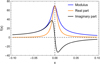Fig. H.1

Sample of the tidal response, plotted in terms of the modulus, real part, and imaginary part of the surface pressure anomaly, all given by Eqs. (H.7). The function f(x) on the y-axis indicates the functional form of the pressure variation, that is, the pressure function divided by the constant factor K. The x-axis is centered at the position of the Lamb resonance. Notable is the difference in the resonant amplification of the response between the real part and the imaginary part.

Next we define the normalized frequency X = σ/σ_L and the dissipation parameter ɛ = σ₀/σ_L ≪ 1, and we rewrite Eq. (H.3) as

$\tilde{δ} p_{s} = K \frac{𝒢 (X)}{ε [(κ + 1) X^{2} - 1] + i X (X^{2} - 1)} .$ $\widetilde \delta {p_{\rm{s}}} = K{{{\cal G}(X)} \over {\varepsilon \left[ {(\kappa + 1){X^2} - 1} \right] + iX\left( {{X^2} - 1} \right)}}.$ (H.6)

The modulus, real part, and the imaginary part of this complex surface pressure oscillation are then straightforwardly deduced as:

$\begin{array}{l} | \tilde{δ} p_{s} | = K \frac{| 𝒢 |}{\sqrt{ε^{2} {[(κ + 1) X^{2} - 1]}^{2} + X^{2} {(X^{2} - 1)}^{2}}}, \\ Re {{\tilde{δ p}}_{s}} = K \frac{ε [(κ + 1) X^{2} - 1] 𝒢_{R} + X (X^{2} - 1) 𝒢_{I}}{ε^{2} {[(κ + 1) X^{2} - 1]}^{2} + X^{2} {(X^{2} - 1)}^{2}}, \\ Im {{\tilde{δ p}}_{s}} = K \frac{ε [(κ + 1) X^{2} - 1] 𝒢_{I} - X (X^{2} - 1) 𝒢_{R}}{ε^{2} {[(κ + 1) X^{2} - 1]}^{2} + X^{2} {(X^{2} - 1)}^{2}}, \end{array}$ $\matrix{ {\left| {\tilde \delta {p_{\rm{s}}}} \right| = K{{|{\cal G}|} \over {\sqrt {{\varepsilon ^2}{{\left[ {(\kappa + 1){X^2} - 1} \right]}^2} + {X^2}{{\left( {{X^2} - 1} \right)}^2}} }},} \hfill \cr {{\mathop{\rm Re}\nolimits} \left\{ {\widetilde \delta {p_{\rm{s}}}} \right\} = K{{\varepsilon \left[ {(\kappa + 1){X^2} - 1} \right]{{\cal G}_{\rm{R}}} + X\left( {{X^2} - 1} \right){{\cal G}_{\rm{I}}}} \over {{\varepsilon ^2}{{\left[ {(\kappa + 1){X^2} - 1} \right]}^2} + {X^2}{{\left( {{X^2} - 1} \right)}^2}}},} \hfill \cr {Im\left\{ {\widetilde \delta {p_{\rm{s}}}} \right\} = K{{\varepsilon \left[ {(\kappa + 1){X^2} - 1} \right]{{\cal G}_{\rm{I}}} - X\left( {{X^2} - 1} \right){{\cal G}_{\rm{R}}}} \over {{\varepsilon ^2}{{\left[ {(\kappa + 1){X^2} - 1} \right]}^2} + {X^2}{{\left( {{X^2} - 1} \right)}^2}}}} \hfill \cr }$ (H.7)

where 𝒢_R = Re{𝒢} and 𝒢_I = Im{𝒢}. In Figure H.1 we plot a sample of the tidal response in terms of the three components, the modulus, the imaginary, and the real part, centered at the resonance. Notable in the figure is the difference between the resonant amplification obtained for the absolute value of the pressure anomaly, or its real part, compared to its imaginary part. Thus one has to be careful in analyzing the tidal amplification induced by the resonance in terms of the surface pressure anomaly compared to its imaginary part, which goes into the computation of the tidal torque.

It is noteworthy that taking Eq. (H.7) in the low frequency limit (X → 0) and setting 𝒢 = 1 we obtain

$Im {\tilde{δ} p_{s}} = K \frac{X}{ε^{2} + X^{2}},$ ${\rm{Im}}\left\{ {\widetilde \delta {p_{\rm{s}}}} \right\} = K{X \over {{\varepsilon ^2} + {X^2}}},$ (H.8)

which is similar to the functional form of the imaginary part of the pressure oscillation given in Ingersoll & Dobrovolskis (1978), and obtained empirically using GCMs in Leconte et al. (2015). This provides the equivalence between the radiative cooling frequency used in our model and the dissipative frequency used in Leconte et al. (2015), as we did in Section 4.1.

Appendix I Moist adiabatic tidal model

In this section, we establish the tidal solution in the case of a moist adiabat rather than the dry adiabat assumed thus far. We show that the moist and dry adiabatic profiles exhibit the same functional form of the tidal response.

For a moist adiabatic temperature profile, the Brunt-Väisälä frequency is expressed as

$N_{B}^{2} = \frac{g}{T_{0}} (\frac{d T_{0}}{d z} + \frac{g}{C_{p} + Δ C_{p}}),$ $N_{\rm{B}}^2 = {g \over {{T_0}}}\left( {{{{\rm{d}}{T_0}} \over {{\rm{d}}z}} + {g \over {{C_p} + {\rm{\Delta }}{C_p}}}} \right),$ (I.1)

where ΔC_p designates the increase of the heat capacity per unit mass due to humidity. As a first approximation, this parameter can be considered to be uniform over the air column. This allows us to introduce the constant parameter κ_M, defined as

$κ_{M} \equiv \frac{R_{s}}{C_{p} + Δ C_{p}},$ ${\kappa _{\rm{M}}} \equiv {{{R_{\rm{s}}}} \over {{C_p} + {\rm{\Delta }}{C_p}}},$ (I.2)

equivalent to the κ parameter characterizing the dry adiabat. We also introduce the ratio q_M, such that 0 < q_M ≤ 1, defined as

$q_{M} \equiv \frac{κ_{M}}{κ},$ ${q_{\rm{M}}} \equiv {{{\kappa _{\rm{M}}}} \over \kappa },$ (I.3)

which quantifies the effect of humidity on the atmospheric structure and tidal waves. Taking the ratio of the slopes of moist (5.9ºC/km) and dry (9.8ºC/km) adiabatic temperature profiles, we get q_M = 0.602 (e.g., Feiccabrino et al. 2015). The Brunt-Väisälä frequency is thus rewritten as

$N_{B}^{2} = \frac{g}{H} (\frac{d \ln H}{d x} + κ_{M}) .$ $N_{\rm{B}}^2 = {g \over H}\left( {{{{\rm{d}}\,\ln H} \over {{\rm{d}}x}} + {\kappa _{\rm{M}}}} \right).$ (I.4)

With these definitions, assuming neutral stratification (N_B = 0) leads to

$H = H_{s} e^{- κ_{M} x} .$ $H = {H_{\rm{s}}}{{\rm{e}}^{ - {\kappa _{\rm{M}}}x}}.$ (I.5)

The other background fields are deduced from H by making use of the hydrostatic approximation and the ideal gas law,

$p_{0} (x) = p_{s} e^{- x}, T_{0} (x) = T_{s} e^{- κ_{M} x}, ρ_{0} (x) = ρ_{s} e^{(κ_{M} - 1) x},$ ${p_0}(x) = {p_{\rm{s}}}{{\rm{e}}^{ - x}},\quad {T_0}(x) = {T_{\rm{s}}}{{\rm{e}}^{ - {\kappa _{\rm{M}}}x}},\quad {\rho _0}(x) = {\rho _{\rm{s}}}{{\rm{e}}^{\left( {{\kappa _{\rm{M}}} - 1} \right)x}},$ (I.6)

with H_s = R_sT_s/g, and ρ_s = p_s/ (gH_s). Written as a function of the altitude, the normalized altitude coordinate x is expressed as

$x = \frac{1}{κ_{M}} \ln (\frac{H_{s}}{H_{s} - κ_{M} z}),$ $x = {1 \over {{\kappa _{\rm{M}}}}}\ln \,\left( {{{{H_{\rm{s}}}} \over {{H_{\rm{s}}} - {\kappa _{\rm{M}}}z}}} \right){\rm{,}}$ (I.7)

and the atmospheric vertical profiles, given in Eq. (13) for the dry adiabat, in the case of a moist adiabat become

$\begin{array}{l} H (z) = H_{s} - κ_{M} z, & p_{0} (z) = p_{s} {(1 - \frac{κ_{M} z}{H_{s}})}^{\frac{1}{κ_{M}}}, \\ T_{0} (z) = T_{s} - \frac{κ_{M} g}{R_{s}} z, & ρ_{0} (z) = \frac{p_{s}}{g H_{s}} {(1 - \frac{κ_{M} z}{H_{s}})}^{\frac{1 - κ_{M}}{κ_{M}}} . \end{array}$ $\matrix{ {H(z) = {H_{\rm{s}}} - {\kappa _{\rm{M}}}z,} \hfill & {{p_0}(z) = {p_{\rm{s}}}{{\left( {1 - {{{\kappa _{\rm{M}}}z} \over {{H_{\rm{s}}}}}} \right)}^{{1 \over {{\kappa _{\rm{M}}}}}}},} \hfill \cr {{T_0}(z) = {T_{\rm{s}}} - {{{\kappa _{\rm{M}}}g} \over {{R_{\rm{s}}}}}z,} \hfill & {{\rho _0}(z) = {{{p_{\rm{s}}}} \over {g{H_{\rm{s}}}}}{{\left( {1 - {{{\kappa _{\rm{M}}}z} \over {{H_{\rm{s}}}}}} \right)}^{{{1 - {\kappa _{\rm{M}}}} \over {{\kappa _{\rm{M}}}}}}}.} \hfill \cr }$ (I.8)

I.1 The wave equation and the tidal solution in the moist adiabatic limit

The humidity of the atmosphere only affects the thermodynamic equation through the modified heat capacity. The thermody-namic equation thus becomes

$(q_{M}^{- 1} - κ) \frac{d p}{d t} - q_{M}^{- 1} g H \frac{d ρ}{d t} = κ ρ_{0} J - ρ_{0} R_{s} σ_{0} δ T .$ $\left( {q_{\rm{M}}^{ - 1} - \kappa } \right){{{\rm{d}}p} \over {{\rm{d}}t}} - q_{\rm{M}}^{ - 1}gH{{{\rm{d}}\rho } \over {{\rm{d}}t}} = \kappa {\rho _0}J - {\rho _0}{R_{\rm{s}}}{\sigma _0}\delta T.$ (I.9)

By introducing the calculation variable G, we rewrite the above equation as

$(q_{M}^{- 1} - κ) G + q_{M}^{- 1} \frac{g H}{p_{0}} \frac{d ρ}{d t} = - κ \frac{ρ_{0}}{p_{0}} J + \frac{ρ_{0} R_{s}}{p_{0}} σ_{0} δ T .$ $\left( {q_{\rm{M}}^{ - 1} - \kappa } \right)G + q_{\rm{M}}^{ - 1}{{gH} \over {{p_0}}}{{{\rm{d}}\rho } \over {{\rm{d}}t}} = - \kappa {{{\rho _0}} \over {{p_0}}}J + {{{\rho _0}{R_{\rm{s}}}} \over {{p_0}}}{\sigma _0}\delta T.$ (I.10)

Finally, we normalize the equations and we switch to the frequency domain. This yields,

$\frac{1}{σ ρ_{0}} \frac{d ρ}{d t} = \partial_{\tilde{t}} \tilde{δ} ρ + \frac{V_{0}}{σ H} \frac{d \ln ρ_{0}}{d x} {\tilde{V}}_{r},$ ${1 \over {\sigma {\rho _0}}}{{{\rm{d}}\rho } \over {{\rm{d}}t}} = {\partial _{\tilde t}}\tilde \delta \rho + {{{V_0}} \over {\sigma H}}{{{\rm{d}}\,\ln {\rho _0}} \over {{\rm{d}}x}}{{\tilde V}_r},$ (I.11)

and the normalized equation for $\tilde{G}$ ${\tilde G}$ ,

$(1 - κ q_{M}) \frac{\tilde{G}}{Γ_{1}} + i \tilde{δ} ρ + η \frac{d \ln ρ_{0}}{d x} {\tilde{V}}_{r} = q_{M} (- \tilde{J} + \frac{δ \tilde{T}}{α}),$ $\left( {1 - \kappa {q_{\rm{M}}}} \right){{\tilde G} \over {{{\rm{\Gamma }}_1}}} + i\tilde \delta \rho + \eta {{{\rm{d}}\,\ln {\rho _0}} \over {{\rm{d}}x}}{{\tilde V}_r} = {q_{\rm{M}}}\left( { - \tilde J + {{\delta \tilde T} \over \alpha }} \right),$ (I.12)

with η = R_p/H and α = σ/σ₀. The structure factors in the tidal equations are expressed as

$\frac{d \ln H}{d x} = \frac{H N_{B}^{2}}{g} - κ_{M}, \frac{d \ln p_{0}}{d x} = - 1,$ ${{{\rm{d}}\,\ln H} \over {{\rm{d}}x}} = {{HN_{\rm{B}}^2} \over g} - {\kappa _{\rm{M}}},\quad {{{\rm{d}}\,\ln {p_0}} \over {{\rm{d}}x}} = - 1,$ (I.13)

and

$\frac{d \ln ρ_{0}}{d x} = - (1 + \frac{d H}{d x}) = - [1 - κ_{M} + \frac{H N_{B}^{2}}{g}] .$ ${{{\rm{d}}\,\ln {\rho _0}} \over {{\rm{d}}x}} = - \left( {1 + {{{\rm{d}}H} \over {{\rm{d}}x}}} \right) = - \left[ {1 - {\kappa _{\rm{M}}} + {{HN_{\rm{B}}^2} \over g}} \right].$ (I.14)

The horizontal structure of the tidal perturbation is obtained similarly as in the other tidal solutions. For the vertical structure, we follow the same steps as in Appendix B. First, the vertical velocity and the temperature variation are eliminated from the thermodynamic equation by making use of Eq. (B.1) and Eq. (B.5), respectively. It follows

$[1 + \frac{d \ln H}{d x} - i \frac{q_{M}}{α}] \tilde{δ} p - (1 - i \frac{q_{M}}{α}) \tilde{δ} ρ = i \frac{H N_{B}^{2}}{g} \tilde{G} - i q_{M} \tilde{J} .$ $\left[ {1 + {{{\rm{d}}\,\ln H} \over {{\rm{d}}x}} - i{{{q_{\rm{M}}}} \over \alpha }} \right]\tilde \delta p - \left( {1 - i{{{q_{\rm{M}}}} \over \alpha }} \right)\tilde \delta \rho = i{{HN_{\rm{B}}^2} \over g}\tilde G - i{q_{\rm{M}}}\tilde J.$ (I.15)

Finally, we use Eq. (B.2) to express $\tilde{δ} ρ$ $\tilde \delta \rho$ as a function of $\tilde{δ} p$ $\tilde \delta p$ and $\tilde{U}$ ${\tilde U}$ , and we end up with

$\partial_{x} \tilde{δ} p = \frac{α}{{(α - i q_{M})}^{- 1}} [i \frac{H N_{B}^{2}}{g} \tilde{G} - \frac{d \ln H}{d x} \tilde{δ} p - i q_{M} \tilde{J}] + \frac{V_{0}^{2}}{g H} \partial_{x} \tilde{U} .$ ${\partial _x}\tilde \delta p = {\alpha \over {{{\left( {\alpha - i{q_{\rm{M}}}} \right)}^{ - 1}}}}\left[ {i{{HN_{\rm{B}}^2} \over g}\tilde G - {{{\rm{d}}\,\ln H} \over {{\rm{d}}x}}\tilde \delta p - i{q_{\rm{M}}}\tilde J} \right] + {{V_0^2} \over {gH}}{\partial _x}\tilde U.$ (I.16)

The equation for $\partial_{x} \tilde{G}$ ${\partial _x}\tilde G$ is the same as in the dry adiabatic case and is given by Eq. (B.8). We thus reformulate the tidal equations as the first order system given by

$\partial_{x} \tilde{G} = A_{1} \tilde{G} + B_{1} \tilde{δ} p + C_{1},$ ${\partial _x}\tilde G = {A_1}\tilde G + {B_1}\tilde \delta p + {C_1},$ (I.17)

$\partial_{x} \tilde{δ} p = A_{2} \tilde{G} + B_{2} \tilde{δ} p + C_{2},$ ${\partial _x}\tilde \delta p = {A_2}\tilde G + {B_2}\tilde \delta p + {C_2},$ (I.18)

with the operators and coefficients

$\begin{array}{l} A_{1} = 1, & A_{2} = i \frac{α H N_{B}^{2}}{g (α - i q_{M})}, \end{array}$ $\matrix{ {{A_1} = 1,} \hfill & {\quad \quad \quad \quad \quad {A_2} = i{{\alpha HN_{\rm{B}}^2} \over {g\left( {\alpha - i{q_{\rm{M}}}} \right)}},} \hfill \cr }$ (I.19)

$\begin{array}{l} B_{1} = - i \frac{g H}{V_{0}^{2}} ℒ, & B_{2} = - \frac{α}{(α - i q_{M})} \frac{d \ln H}{d x}, \end{array}$ $\matrix{ {{B_1} = - i{{gH} \over {V_0^2}}{\cal L},} \hfill & {\quad \quad \quad \quad {B_2} = - {\alpha \over {\left( {\alpha - i{q_{\rm{M}}}} \right)}}{{{\rm{d}}\,\ln H} \over {{\rm{d}}x}},} \hfill \cr }$ (I.20)

$C_{1} = i (ℒ - \frac{V_{0}^{2}}{g H} \partial_{x}) \tilde{U}, C_{2} = \frac{V_{0}^{2}}{g H} \partial_{x} \tilde{U} - \frac{i α q_{M} \tilde{J}}{α - i q_{M}} .$ ${C_1} = i\,\left( {{\cal L} - {{V_0^2} \over {gH}}{\partial _x}} \right)\,\tilde U,\quad \quad {C_2} = {{V_0^2} \over {gH}}{\partial _x}\tilde U - {{i\alpha {q_{\rm{M}}}\tilde J} \over {\alpha - i{q_{\rm{M}}}}}.$ (I.21)

This system is reduced to a single second order equation of $\tilde{G}$ ${\tilde G}$ in the form given by Eq. (B.11) but with the modified operators A, B, and C given by

$A = - 1 + \frac{i q_{M}}{α - i q_{M}} \frac{d \ln H}{d x},$ $A = - 1 + {{i{q_{\rm{M}}}} \over {\alpha - i{q_{\rm{M}}}}}{{{\rm{d}}\,\ln H} \over {{\rm{d}}x}},$ (I.22)

$B = - \frac{α}{(α - i q_{M})} [\frac{i}{α} q_{M} \frac{d \ln H}{d x} + \frac{H^{2} N_{B}^{2}}{V_{0}^{2}} ℒ],$ $B = - {\alpha \over {\left( {\alpha - i{q_{\rm{M}}}} \right)}}\left[ {{i \over \alpha }{q_{\rm{M}}}{{{\rm{d}}\,\ln H} \over {{\rm{d}}x}} + {{{H^2}N_{\rm{B}}^2} \over {V_0^2}}{\cal L}} \right],$ (I.23)

$\begin{array}{l} C = - \frac{g H α q_{M}}{V_{0}^{2} (α - i q_{M})} ℒ \tilde{J} \\ - [\frac{q_{M}}{α - i q_{M}} \frac{d \ln H}{d x} (ℒ - \frac{V_{0}^{2}}{g H} \frac{d}{d x}) + i \frac{d}{d x} (\frac{V_{0}^{2}}{g H} \frac{d}{d x})] \tilde{U} . \end{array}$ $\matrix{ {C = - {{gH\alpha {q_{\rm{M}}}} \over {V_0^2\left( {\alpha - i{q_{\rm{M}}}} \right)}}{\cal L}\tilde J} \hfill \cr {\,\,\,\,\,\,\,\,\,\,\, - \left[ {{{{q_{\rm{M}}}} \over {\alpha - i{q_{\rm{M}}}}}{{{\rm{d}}\,\ln H} \over {{\rm{d}}x}}\left( {{\cal L} - {{V_0^2} \over {gH}}{{\rm{d}} \over {{\rm{d}}x}}} \right) + i{{\rm{d}} \over {{\rm{d}}x}}\left( {{{V_0^2} \over {gH}}{{\rm{d}} \over {{\rm{d}}x}}} \right)} \right]\tilde U.} \hfill \cr }$ (I.24)

The wave equation is finally written in its classical form by substituting ℒ = −Λ_n and introducing the change of variable $ℒ = - Λ_{n}$ ${\cal L} = - {{\rm{\Lambda }}_n}$ ,

$\frac{d^{2} Ψ}{d x^{2}} + k_{n}^{2} Ψ = ϕ^{- 1} C,$ ${{{d^2}{\rm{\Psi }}} \over {d{x^2}}} + k_n^2{\rm{\Psi }} = {\phi ^{ - 1}}C,$ (I.25)

with ϕ being expressed as

$ϕ (x) = \exp [\frac{x}{2} - \frac{1}{2} \int_{0}^{x} \frac{i q_{M}}{α - i q_{M}} (\frac{H N_{B}^{2}}{g} - κ q_{M}) d x],$ $\phi (x) = \exp \,\left[ {{x \over 2} - {1 \over 2}\int_0^x {{{i{q_{\rm{M}}}} \over {\alpha - i{q_{\rm{M}}}}}\left( {{{HN_{\rm{B}}^2} \over g} - \kappa {q_{\rm{M}}}} \right)\,dx} } \right]\,,$ (I.26)

and the squared vertical wavenumber as

$\begin{array}{l} k_{n}^{2} = - \frac{1}{4} {{(1 - \frac{i q_{M}}{α - i q_{M}} \frac{d \ln H}{d x})}^{2} + 2 \frac{d}{d x} (\frac{i q_{M}}{α - i q_{M}} \frac{d \ln H}{d x}) \\ - \frac{4 α}{α - i q_{M}} [\frac{g H Λ_{n}}{V_{0}^{2}} (\frac{d \ln H}{d x} + κ q_{M}) - i α q_{M} \frac{d \ln H}{d x}]}, \end{array}$ $\matrix{ {k_n^2 = - {1 \over 4}\left\{ {{{\left( {1 - {{i{q_{\rm{M}}}} \over {\alpha - i{q_{\rm{M}}}}}{{{\rm{d}}\,\ln H} \over {{\rm{d}}x}}} \right)}^2} + 2{{\rm{d}} \over {{\rm{d}}x}}\left( {{{i{q_{\rm{M}}}} \over {\alpha - i{q_{\rm{M}}}}}{{{\rm{d}}\,\ln H} \over {{\rm{d}}x}}} \right)} \right.} \hfill \cr {\,\,\,\,\,\,\,\,\,\,\,\left. {\,\,\, - {{4\alpha } \over {\alpha - i{q_{\rm{M}}}}}\left[ {{{gH{{\rm{\Lambda }}_n}} \over {V_0^2}}\left( {{{{\rm{d}}\,\ln H} \over {{\rm{d}}x}} + \kappa {q_{\rm{M}}}} \right) - i\alpha {q_{\rm{M}}}{{{\rm{d}}\,\ln H} \over {{\rm{d}}x}}} \right]} \right\},} \hfill \cr }$ (I.27)

Thus far, we have not implemented the neutral stratification assumption (N_B = 0). In doing so, and considering the thermal tide solely (Ũ = 0), the components of the wave equation simplify to

$A = - \frac{α + i q_{M} (q_{M} κ - 1)}{α - i q_{M}},$ $A = - {{\alpha + i{q_{\rm{M}}}\left( {{q_{\rm{M}}}\kappa - 1} \right)} \over {\alpha - i{q_{\rm{M}}}}},$ (I.28)

$B = \frac{i q_{M}^{2} κ}{α - i q_{M}},$ $B = {{iq_{\rm{M}}^2\kappa } \over {\alpha - i{q_{\rm{M}}}}},$ (I.29)

$C = \frac{g α H q_{M} Λ_{n}}{V_{0}^{2} (α - i q_{M})} \tilde{J},$ $C = {{g\alpha H{q_{\rm{M}}}{{\rm{\Lambda }}_n}} \over {V_0^2\left( {\alpha - i{q_{\rm{M}}}} \right)}}\tilde J,$ (I.30)

$ϕ (x) = \exp [- \frac{A}{2} x],$ $\phi (x) = \exp \,\left[ { - {A \over 2}x} \right],$ (I.31)

$k_{n}^{2} = {[\frac{i α + q_{M} + q_{M} κ}{2 (α - i q_{M})}]}^{2} .$ $k_n^2 = {\left[ {{{i\alpha + {q_{\rm{M}}} + {q_{\rm{M}}}\kappa } \over {2\left( {\alpha - i{q_{\rm{M}}}} \right)}}} \right]^2}.$ (I.32)

It is now straightforward to obtain the tidal solution in the moist adiabatic limit following the same recipe we implemented in the dry adiabatic limit. For the vertical profile of the pressure perturbation we obtain

$\begin{array}{l} \tilde{δ} p (x) = \frac{i K q_{M} e^{q_{M} κ x}}{b_{J} (X - i ε q_{M}) + i ε q_{M}^{2} κ} {(b_{J} + 1) e^{- b_{J} x} \\ + \frac{[1 - (1 + b_{J}) X^{2}] [X - i ε q_{M} (1 + q_{M} κ)]}{(X - i ε q_{M}) (X^{2} - 1) - i ε q_{M}^{2} κ X^{2}} e^{(i k_{n} - \frac{A}{2}) x}} . \end{array}$ $\matrix{ {\tilde \delta p(x) = {{iK{q_{\rm{M}}}{{\rm{e}}^{{q_{\rm{M}}}\kappa x}}} \over {{b_{\rm{J}}}\left( {X - i\varepsilon {q_{\rm{M}}}} \right) + i\varepsilon q_{\rm{M}}^2\kappa }}\left\{ {\left( {{b_{\rm{J}}} + 1} \right){{\rm{e}}^{ - {b_{\rm{J}}}x}}} \right.} \hfill \cr {\,\,\,\,\,\,\,\,\,\,\,\,\,\,\,\,\,\,\,\,\left. {\,\, + {{\left[ {1 - \left( {1 + {b_{\rm{J}}}} \right){X^2}} \right]\,\left[ {X - i\varepsilon {q_{\rm{M}}}\left( {1 + {q_{\rm{M}}}\kappa } \right)} \right]} \over {\left( {X - i\varepsilon {q_{\rm{M}}}} \right)\,\left( {{X^2} - 1} \right) - i\varepsilon q_{\rm{M}}^2\kappa {X^2}}}{{\rm{e}}^{\left( {i{k_n} - {A \over 2}} \right)x}}} \right\}.} \hfill \cr }$ (I.33)

with K being the dimensionless constant defined by Eq. (H.5) for a dry adiabat, and e and X are defined as in Appendix H. Thus the appearance of q_M in the common factor of the latter equation renders the dependence of the tidal response on humidity explicit. Finally, the surface pressure perturbation (x = 0) is readily deduced from the above expression in the form

$\tilde{δ} p_{s} = \frac{K q_{M}}{q_{M} ε [(1 + κ q_{M}) X^{2} - 1] + i X (X^{2} - 1)} .$ $\tilde \delta {p_{\rm{s}}} = {{K{q_{\rm{M}}}} \over {{q_{\rm{M}}}\varepsilon \left[ {\left( {1 + \kappa {q_{\rm{M}}}} \right){X^2} - 1} \right] + iX\,\left( {{X^2} - 1} \right)}}.$ (I.34)

We observe that switching from the dry adiabat to the moist adiabat amounts to replacing everywhere κ by κ_M, and ɛ by q_Mɛ. The functional form of the solution is the same in both cases. Consequently, the resonant frequency in the moist adiabatic limit is exactly equal to that in the dry adiabatic limit, and so is the resonant LOD. Moreover, the normalizing factor at the numerator of Eq. (I.34) is reduced by the factor q_M as is the dissipation parameter ϵ. Therefore, the amplification factor which scales as the ratio of the two is barely affected by the humidity of the atmosphere.

Appendix J Estimates of the absorbed tidal energy

In this section, we compute estimates of the atmospheric opacity parameter α_A. As defined in the main text (Section 2.2), α_A quantifies the fraction of thermal energy that is absorbed by the atmosphere and is actually available for semidiurnal thermotidal dynamics. To our knowledge, this input tidal power is rarely evaluated in the literature. Here we show that it can be estimated from the distributions of heating rates that are measured in the Earth’s atmosphere or computed using GCM simulations. We refer in what follows to Chapman & Lindzen (1970) and Vichare & Rajaram (2013) who provide such distributions for water vapor (H₂O) and ozone (O₃).

First, we consider the vertical and latitudinal profiles shown by Chapman & Lindzen (1970). These profiles do not directly quantify the heating rate J, but rather the equivalent temperature variation τ_G, which approximately corresponds to the temperature oscillation produced by J^m,σ. The input power is thus defined as (Chapman & Lindzen 1970, Eqs. (143-144))

$J = Re {\sum_{σ} \sum_{m} J^{m, σ} (x, θ, φ) e^{i σ t}},$ $J = {\mathop{\rm Re}\nolimits} \,\left\{ {\mathop \sum \limits_\sigma \mathop \sum \limits_m {J^{m,\sigma }}(x,\theta ,\varphi ){e^{i\sigma t}}} \right\},$ (J.1)

with the coefficients J^m,σ given by

$J^{m, σ} (x, θ, φ) = i σ C_{p} τ_{G}^{m} σ (x, θ, φ),$ ${J^{m,\sigma }}(x,\theta ,\varphi ) = i\sigma {C_{\rm{p}}}\tau _{\rm{G}}^m\sigma (x,\theta ,\varphi ),$ (J.2)

where the heat capacity of the gas per unit mass C_p = ℛ_s/κ. Figure 3.2 of Chapman & Lindzen (1970) shows the normalized vertical distribution of $τ_{G}^{2, σ}$ $\tau _{\rm{G}}^{2,\sigma }$ . Following the authors (their Eq. 163), we set H = 7.6 km. The semidiurnal distributions of $τ_{G}^{2, σ}$ $\tau _{\rm{G}}^{2,\sigma }$ for water vapor and ozone can be approximated by the functions

$τ_{G, H_{2} O} (x, θ, φ) = T_{H_{2} O} V_{H_{2} O} (x) \sin θ e^{i 2 φ},$ ${\tau _{{\rm{G}},{{\rm{H}}_2}{\rm{O}}}}(x,\theta ,\varphi ) = {T_{{{\rm{H}}_2}{\rm{O}}}}{V_{{{\rm{H}}_2}{\rm{O}}}}(x)\sin \theta {e^{i2\varphi }},$ (J.3)

$τ_{G, O_{3}} (x, θ, φ) = T_{O_{3}} V_{O_{3}} (x) \sin^{2} θ e^{i 2 φ},$ ${\tau _{{\rm{G}},{{\rm{O}}_3}}}(x,\theta ,\varphi ) = {T_{{{\rm{O}}_3}}}{V_{{{\rm{O}}_3}}}(x){\sin ^2}\theta {e^{i2\varphi }},$ (J.4)

with $T_{H_{2} O} = 0.035 K$ ${T_{{{\rm{H}}_2}{\rm{O}}}} = 0.035\,\,{\rm{K}}$ and $T_{O_{3}} = 0.25 K$ ${T_{{{\rm{O}}_3}}} = 0.25\,\,{\rm{K}}$ . As the vertical profile of water vapor shown by Figure 3.2 of Chapman & Lindzen (1970) is an exponentially decaying function of the altitude, the function $V_{H_{2} O}$ ${V_{{{\rm{H}}_2}{\rm{O}}}}$ of Eq.(J.3) is set to

$V_{H_{2} O} (x) = e^{- k_{H_{2} O} x},$ ${V_{{{\rm{H}}_2}{\rm{O}}}}(x) = {e^{ - {k_{{{\rm{H}}_2}{\rm{O}}}}x}},$ (J.5)

where $k_{H_{2} O} \approx 1 / 3$ ${k_{{{\rm{H}}_2}{\rm{O}}}} \approx 1/3$ . Similarly, the vertical profile of ozone absorption can be approximated by a truncated sine function,

$V_{O_{3}} (x) = {\begin{array}{l} K_{O_{3}} \sin (\frac{π (x - x_{1})}{x_{2} - x_{1}}), & x_{1} \leq x \leq x_{2}, \\ 0 & elsewhere, \end{array}$ ${V_{{{\rm{O}}_3}}}\left( x \right) = \left\{ {\matrix{ {{K_{{{\rm{O}}_3}}}\sin \,\left( {{{\pi \left( {x - {x_1}} \right)} \over {{x_2} - {x_1}}}} \right),} \hfill & {{x_1} \le x \le {x_2},} \hfill \cr 0 \hfill & {{\rm{elsewhere}},} \hfill \cr } } \right.$ (J.6)

with $K_{O_{3}} = 1.4$ ${K_{{{\rm{O}}_3}}} = 1.4$ , x₁ = z₁/H, and x₂ = z₂/H, the altitudes z₁ and z₂ being set to z₁ = 18 km and z₂ = 78 km. At a given location on the sphere (θ, φ), the total flux absorbed by the atmosphere for the spherical harmonic Y₂₂ is defined as

$δ ℱ (θ, φ) = δ ℱ_{22} Y_{22} (θ, φ) .$ $\delta {\cal F}(\theta ,\varphi ) = \delta {{\cal F}_{22}}{Y_{22}}(\theta ,\varphi ).$ (J.7)

The efficiency parameter α_A of our model is basically the ratio between δℱ₂₂ and the corresponding component of the incident Solar flux, which we retrieve in Appendix E (Eq. E.13) as

$δ F_{22} = \frac{\sqrt{30 π}}{16} F_{⋆} .$ $\delta {F_{22}} = {{\sqrt {30\pi } } \over {16}}{F_ \star }.$ (J.8)

In order to simplify calculations, we assume that the latitudinal profile of ozone can be approximated by the function sin² θ, similar to the latitudinal profile of water vapor. Under this assumption, we rewrite Eqs.(J.3) and (J.4) as

$τ_{G, H_{2} O} (x, θ, φ) = \frac{4}{3} \sqrt{\frac{6 π}{5}} T_{H_{2} O} V_{H_{2} O} (x) Y_{22} (θ, φ),$ ${\tau _{{\rm{G}},{{\rm{H}}_2}{\rm{O}}}}(x,\theta ,\varphi ) = {4 \over 3}\sqrt {{{6\pi } \over 5}} {T_{{{\rm{H}}_2}{\rm{O}}}}{V_{{{\rm{H}}_2}{\rm{O}}}}(x){Y_{22}}(\theta ,\varphi ),$ (J.9)

$τ_{G, O_{3}} (x, θ, φ) = \frac{4}{3} \sqrt{\frac{6 π}{5}} T_{O_{3}} V_{O_{3}} (x) Y_{22} (θ, φ),$ ${\tau _{{\rm{G}},{{\rm{O}}_3}}}(x,\theta ,\varphi ) = {4 \over 3}\sqrt {{{6\pi } \over 5}} {T_{{{\rm{O}}_3}}}{V_{{{\rm{O}}_3}}}(x){Y_{22}}(\theta ,\varphi ),$ (J.10)

and the corresponding heating rates as

$J_{H_{2} O} (x, θ, φ) = \frac{4}{3} \sqrt{\frac{6 π}{5}} σ C_{p} T_{H_{2} O} V_{H_{2} O} (x) Y_{22} (θ, φ),$ ${J_{{{\rm{H}}_2}{\rm{O}}}}(x,\theta ,\varphi ) = {4 \over 3}\sqrt {{{6\pi } \over 5}} \sigma {C_{\rm{p}}}{T_{{{\rm{H}}_2}{\rm{O}}}}{V_{{{\rm{H}}_2}{\rm{O}}}}(x){Y_{22}}(\theta ,\varphi ),$ (J.11)

$J_{O_{3}} (x, θ, φ) = \frac{4}{3} \sqrt{\frac{6 π}{5}} σ C_{p} T_{O_{3}} V_{O_{3}} (x) Y_{22} (θ, φ),$ ${J_{{{\rm{O}}_3}}}(x,\theta ,\varphi ) = {4 \over 3}\sqrt {{{6\pi } \over 5}} \sigma {C_{\rm{p}}}{T_{{{\rm{O}}_3}}}{V_{{{\rm{O}}_3}}}(x){Y_{22}}(\theta ,\varphi ),$ (J.12)

where the imaginary number appearing in Eq.(J.2) has been ignored since it does not affectthe amplitude of the thermal forc-ing⁹. For a given component, the total input power is obtained by integrating the heating rate over the air column

$δ ℱ = \int_{0}^{+ \infty} J ρ_{0} H d x = \frac{p_{s}}{g} \int_{0}^{+ \infty} J e^{- x} d x,$ $\delta {\cal F} = \int_0^{ + \infty } {J{\rho _0}Hdx = {{{p_{\rm{s}}}} \over g}} \int_0^{ + \infty } {J{e^{ - x}}dx} ,$ (J.13)

noting that ρ₀H = (p₀/g). This requires computing the integral of the vertical distribution of the heating rates,

$A_{H_{2} O} = \int_{0}^{+ \infty} V_{H_{2} O} e^{- x} d x = \frac{1}{1 + k_{H_{2} O}},$ ${A_{{{\rm{H}}_2}{\rm{O}}}} = \int_0^{ + \infty } {{V_{{{\rm{H}}_2}{\rm{O}}}}{e^{ - x}}dx = {1 \over {1 + {k_{{{\rm{H}}_2}{\rm{O}}}}}}} ,$ (J.14)

$\begin{array}{l} A_{O_{3}} = \int_{0}^{+ \infty} V_{O_{3}} e^{- x} d x \\ = K_{O_{3}} π \frac{(x_{2} - x_{1}) (e^{- x_{1}} + e^{- x_{2}})}{π^{2} + {(x^{2} - x_{1})}^{2}} . \end{array}$ $\matrix{ {{A_{{{\rm{O}}_3}}} = \int_0^{ + \infty } {{V_{{{\rm{O}}_3}}}{e^{ - x}}dx} } \hfill \cr {\,\,\,\,\,\,\,\,\,\, = {K_{{{\rm{O}}_3}}}\pi {{\left( {{x_2} - {x_1}} \right)\,\left( {{e^{ - {x_1}}} + {e^{ - {x_2}}}} \right)} \over {{\pi ^2} + {{\left( {{x^2} - {x_1}} \right)}^2}}}.} \hfill \cr }$ (J.15)

We end up with $A_{H_{2} O} = 0.75$ ${A_{{{\rm{H}}_2}{\rm{O}}}} = 0.75$ and $A_{O_{3}} = 4.5 \times 10^{- 2}$ ${A_{{{\rm{O}}_3}}} = 4.5 \times {10^{ - 2}}$ . Therefore, the total fluxes absorbed by water vapor and ozone are given by

$δ F_{H_{2} O} (θ, φ) = δ ℱ_{H_{2} O; 22} Y_{22} (θ, φ),$ $\delta {F_{{{\rm{H}}_2}{\rm{O}}}}(\theta ,\varphi ) = \delta {{\cal F}_{{{\rm{H}}_2}{\rm{O}};22}}{Y_{22}}(\theta ,\varphi ),$ (J.16)

$δ F_{O_{3}} (θ, φ) = δ ℱ_{O_{3}; 22} Y_{22} (θ, φ),$ $\delta {F_{{{\rm{O}}_3}}}(\theta ,\varphi ) = \delta {{\cal F}_{{{\rm{O}}_3};22}}{Y_{22}}(\theta ,\varphi ),$ (J.17)

with the components

$δ ℱ_{H_{2} O; 22} = \frac{4}{3} \sqrt{\frac{6 π}{5}} σ C_{p} \frac{p_{s}}{g} T_{H_{2} O} A_{H_{2} O},$ $\delta {{\cal F}_{{{\rm{H}}_2}{\rm{O}};22}} = {4 \over 3}\sqrt {{{6\pi } \over 5}} \sigma {C_{\rm{p}}}{{{p_{\rm{s}}}} \over g}{T_{{{\rm{H}}_2}{\rm{O}}}}{A_{{{\rm{H}}_2}{\rm{O}}}},$ (J.18)

$δ ℱ_{O_{3}; 22} = \frac{4}{3} \sqrt{\frac{6 π}{5}} σ C_{p} \frac{p_{s}}{g} T_{O_{3}} A_{O_{3}} .$ $\delta {{\cal F}_{{{\rm{O}}_3};22}} = {4 \over 3}\sqrt {{{6\pi } \over 5}} \sigma {C_{\rm{p}}}{{{p_{\rm{s}}}} \over g}{T_{{{\rm{O}}_3}}}{A_{{{\rm{O}}_3}}}.$ (J.19)

Using σ = 1.45 × 10⁻⁴ s⁻¹, C_p = 1004.7 J kg⁻¹ K⁻¹, p_s = 1013.25 hPa, g = 9.81 m s⁻², and F_⋆ = 1366 W m⁻², we obtain δF₂₂ = 828.8 W m⁻², and

$\begin{array}{l} δ ℱ_{H_{2} O; 22} \approx 102 W m^{- 2}, & \frac{δ ℱ_{H_{2} O; 22}}{δ F_{22}} \approx 12.3 %, \\ δ ℱ_{O_{3}; 22} \approx 44 W m^{- 2}, & \frac{δ ℱ_{O_{3}; 22}}{δ F_{22}} \approx 5.3 %, \\ δ ℱ_{tot; 22} \approx 146 W m^{- 2}, & \frac{δ ℱ_{tot; 22}}{δ F_{22}} \approx 17.6 % . \end{array}$ $\matrix{ {\delta {{\cal F}_{{{\rm{H}}_2}{\rm{O}};22}} \approx 102\,{\rm{W}}\,{{\rm{m}}^{ - 2}},} \hfill & {\quad \quad \quad {{\delta {{\cal F}_{{{\rm{H}}_2}{\rm{O}};22}}} \over {\delta {F_{22}}}} \approx 12.3{\rm{\% }},} \hfill \cr {\delta {{\cal F}_{{{\rm{O}}_3};22}} \approx 44\,{\rm{W}}\,{{\rm{m}}^{ - 2}},} \hfill & {\quad \quad \quad {{\delta {{\cal F}_{{{\rm{O}}_3};22}}} \over {\delta {F_{22}}}} \approx 5.3{\rm{\% }},} \hfill \cr {\delta {{\cal F}_{{\rm{tot}};22}} \approx 146\,{\rm{W}}\,{{\rm{m}}^{ - 2}},} \hfill & {\quad \quad \quad {{\delta {{\cal F}_{{\rm{tot}};22}}} \over {\delta {F_{22}}}} \approx 17.6{\rm{\% }}{\rm{.}}} \hfill \cr }$ (J.20)

Similar estimates can be computed from the profiles shown by Vichare & Rajaram (2013) (see their Figure 4), where the heating rate is plotted as a function of altitude for the main Hough functions structuring the semi-diurnal atmospheric tide on Earth. Without elucidating again the copious details of the procedure, we obtain for the profiles in Vichare & Rajaram (2013) the following:

$\begin{array}{l} δ ℱ_{H_{2} O; 22} \approx 116 W m^{- 2}, & \frac{δ ℱ_{H_{2} O; 22}}{δ F_{22}} \approx 14.0 %, \\ δ ℱ_{O_{3}; 22} \approx 34 W m^{- 2}, & \frac{δ ℱ_{O_{3}; 22}}{δ F_{22}} \approx 4.2 %, \\ δ ℱ_{tot; 22} \approx 150 W m^{- 2}, & \frac{δ ℱ_{tot; 22}}{δ F_{22}} \approx 18.1 % . \end{array}$ $\matrix{ {\delta {{\cal F}_{{{\rm{H}}_2}{\rm{O}};22}} \approx 116\,{\rm{W}}\,{{\rm{m}}^{ - 2}},} \hfill & {\quad \quad \quad {{\delta {{\cal F}_{{{\rm{H}}_2}{\rm{O}};22}}} \over {\delta {F_{22}}}} \approx 14.0{\rm{\% }},} \hfill \cr {\delta {{\cal F}_{{{\rm{O}}_3};22}} \approx 34\,{\rm{W}}\,{{\rm{m}}^{ - 2}},} \hfill & {\quad \quad \quad {{\delta {{\cal F}_{{{\rm{O}}_3};22}}} \over {\delta {F_{22}}}} \approx 4.2{\rm{\% }},} \hfill \cr {\delta {{\cal F}_{{\rm{tot}};22}} \approx 150\,{\rm{W}}\,{{\rm{m}}^{ - 2}},} \hfill & {\quad \quad \quad {{\delta {{\cal F}_{{\rm{tot}};22}}} \over {\delta {F_{22}}}} \approx 18.1{\rm{\% }}{\rm{.}}} \hfill \cr }$ (J.21)

Put together, these computed estimates are consistent and suggest that the efficiency parameter is around α_A~17–18%, which is close to the constraint on α_A (14%, Section 4.1) obtained by fitting our model parameters to reproduce the present-day semidiurnal surface pressure variations.

Appendix K Benchmarking our model against GCM simulations

The work of Auclair-Desrotour et al. (2019) presents, to our knowledge, the only attempt on recovering the tidal torque exerted about the spin axis of a thermally forced atmosphere in the high frequency regime, namely, the regime where the Lamb resonance is encountered, using GCM simulations. Specifically, the mentioned work computed the tidal torque from 3D simulations of atmospheric dynamics using the generic version of the LMDZ GCM (Hourdin et al. 2006) in the case of a nitrogen dominated atmosphere around a dry rocky Venus-like planet.

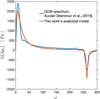Fig. K.1

Similar to Figure 2, the tidal spectra, in terms of the imaginary part of the surface pressure anomaly, are plotted as a function of the normalized tidal frequency ω. The blue curve is that computed numerically in Auclair-Desrotour et al. (2019) using 3D GCM simulations, while the orange curve is recovered from our model by tuning the two free frequencies σ_bl and σ₀ as discussed in Appendix K.

Imposing on our analytical solution (Eq.22) the same planetary parameters defined in Table 1 of Auclair-Desrotour et al. (2019), for a 10 bar atmosphere, and setting σ_bl = 10⁻⁵ s⁻¹ and σ₀ = 4 × 10⁻⁶ s⁻¹, we recover in Figure K.1 a tidal spectrum that reasonably fits the GCM computed spectrum. In particular, we recover the two amplified responses of the torque in the vicinity of synchronization and at the Lamb resonance, and we recover the asymmetry in the Lamb resonance where the positive peak of the torque is annihilated. Furthermore, we recover a similar scaling of the torque with the forcing frequency σ. Namely, for the GCM spectrum, the tidal torque 𝒯 ∝ σ^0.75 near synchronization, and in the high frequency regime 𝒯 ∝ σ⁻¹; while for our model, 𝒯 ∝ σ^0.53 in the former regime, and 𝒯 ∝ σ⁻¹ in the latter.

Appendix L Atmospheric compositional variations and the possible interplay between shortwave and longwave heating

When studying the case of the Earth in the main text, we have assumed that the atmosphere is always heated by the shortwave. We have thus ignored the asynchronous heating in the infrared, which, as we showed in Section 3.2, breaks the symmetry of the Lamb resonance by attenuating the accelerative peak of the tidal torque. The results obtained for the amplitude of the accelerative tidal torque at the resonance can thus be considered as the optimistic limit of the resonant amplitude, as the latter can be attenuated once the longwave heating starts to play a significant role. However, an additional attenuation effect is delivered by the more efficient radiative cooling on a warmer Earth. Namely, the radiative cooling frequency features a strong temperature dependence that scales as σ₀ ∝ T³. Henceforth, the temperature increase required to place the resonance occurrence in the Precambrian would also attenuated the resonant amplitude of the torque by increasing σ₀. Here we intend to elaborate further on this signature, which is driven by atmospheric compositional variations, by studying the functional form of the tidal response obtained in Appendix H.

The form of the pressure anomaly in Eqs. (H.7) allows for an analytical investigation of the Lamb resonance. Namely, we can characterize the positive and negative peaks of the resonance by studying the derivative of the imaginary part of the pressure anomaly. We focus on the limit studied for the Earth in the main text and set 𝒢 = 1, that is, we assume thermotidal heating is dominated by direct shortwave absorption. Computing the roots of the derivative of Eq. (H.7) and substituting them in the expression, we obtain the amplitude of the peaks around the resonance. Namely, we denote by η the ratio between the value of the tidal torque reached at the peaks around resonance to that at present. Considering the predominant terms of the obtained roots, this amplification ratio reads as

$η \approx \frac{K_{⊘}}{K_{\oplus}} \frac{ε_{\oplus}}{ε_{⊘}} η_{\oplus},$ $\eta \approx {{{K_ \oslash }} \over {{K_ \oplus }}}{{{\varepsilon _ \oplus }} \over {{\varepsilon _ \oslash }}}{\eta _ \oplus },$ (L.1)

where we have denoted by the subscript ⊘ the parameter values at the resonance, in contrast with the present values denoted by ⊕.

Now we allow for variations in K that are induced by the parameters entering into the definition of Eq. (H.5). Namely, presuming that κ, R_p, g, and Λ₂ are indeed constant, the rest of the parameters would modify the expression of the amplification factor ŋ (Eq. L.1) into:

$η = η_{\oplus} (\frac{α_{A; ⊘}}{α_{A; \oplus}}) (\frac{F_{⋆; ⊘}}{F_{⋆ : \oplus}}) (\frac{p_{s; \oplus}}{p_{s; ⊘}}) {(\frac{σ_{L; \oplus}}{σ_{L; ⊘}})}^{2} (\frac{σ_{0; \oplus}}{σ_{0; ⊘}}) .$ $\eta = {\eta _ \oplus }\left( {{{{\alpha _{{\rm{A}};\emptyset }}} \over {{\alpha _{{\rm{A}}; \oplus }}}}} \right)\,\left( {{{{F_{ \star ;\emptyset }}} \over {{F_{ \star : \oplus }}}}} \right)\,\left( {{{{p_{{\rm{s}}; \oplus }}} \over {{p_{{\rm{s}};\emptyset }}}}} \right)\,{\left( {{{{\sigma _{{\rm{L}}; \oplus }}} \over {{\sigma _{{\rm{L}};\emptyset }}}}} \right)^2}\,\left( {{{{\sigma _{0; \oplus }}} \over {{\sigma _{0;\emptyset }}}}} \right)\,.$ (L.2)

The resonant frequency in the adiabatic limit scales as $σ_{L} \propto T_{s}^{1 / 2}$ ${\sigma _{\rm{L}}} \propto T_{\rm{s}}^{1/2}$ . Moreover, the radiative cooling frequency is also a function of the surface temperature and it scales as $σ_{0} \propto p_{s}^{- 1} T_{s}^{3}$ ${\sigma _0} \propto p_{\rm{s}}^{ - 1}T_{\rm{s}}^3$ (e.g., Eq. 10 of Showman & Guillot 2002). Including these scaling relationships in the latter expression of the amplification factor one finds that

$η = η_{\oplus} (\frac{α_{A; ⊘}}{α_{A; \oplus}}) (\frac{F_{⋆; ⊘}}{F_{⋆ : \oplus}}) {(\frac{T_{s; \oplus}}{T_{s; ⊙}})}^{4} .$ $\eta = {\eta _ \oplus }\left( {{{{\alpha _{{\rm{A}};\emptyset }}} \over {{\alpha _{{\rm{A}}; \oplus }}}}} \right)\,\left( {{{{F_{ \star ;\emptyset }}} \over {{F_{ \star : \oplus }}}}} \right)\,{\left( {{{{T_{{\rm{s}}; \oplus }}} \over {{T_{{\rm{s}}; \odot }}}}} \right)^4}.$ (L.3)

The equilibrium surface temperature varies as T_s ∝ (α_hF_⋆)^1/4, where α_h is the fraction of flux that is absorbed by the atmosphere, mainly in the infrared absorption. It follows that

$η = η_{\oplus} (\frac{α_{A; ⊘}}{α_{A; \oplus}}) (\frac{α_{h; \oplus}}{α_{h; ⊘}}) .$ $\eta = {\eta _ \oplus }\left( {{{{\alpha _{{\rm{A}};\emptyset }}} \over {{\alpha _{{\rm{A}}; \oplus }}}}} \right)\,\left( {{{{\alpha _{{\rm{h}}; \oplus }}} \over {{\alpha _{{\rm{h}};\emptyset }}}}} \right)\,.$ (L.4)

This interesting and simplified version of the amplification factor shows that η depends on the opacity of the atmosphere in the visible (via α_A) and in the infrared (via α_h), which are functions of the composition. Namely, the two absorption coefficients have opposite effects on η: a past atmosphere that is more opaque in the visible features a greater amplification factor, and thus prompts a stronger tidal response upon the resonance occurrence. In contrast, a larger past opacity in the infrared tends to attenuate the resonance amplified response. Thus the bottom line is, increased greenhouse gases in the past (mainly CO₂), tend to decrease the amplitude of the accelerative resonant response of the atmosphere via, first, Eq. (L.4), and via increasing the contribution of the asynchronous thermotidal heating that induces a phase lag on the tidal bulge and consequently attenuates the accelerative torque around the resonance.

Appendix M The resonant period in the isothermal limit

Here we discuss the limit where the temperature profile of the atmosphere is modeled by an isotherm, in contrast with the adi-abatic profile we assume in our neutrally stratified model. The isothermal limit translates to a positive and constant value of the Brunt–Väisälä frequency N_B, and it has been studied earlier using the linear theory of atmospheric tides (e.g., Lindzen 1978; Lindzen & Blake 1972; Auclair-Desrotour et al. 2019). We are specifically interested in estimating the difference between the two models in terms of the Lamb resonance period. Namely, we aim to define the spectral position of the resonance in the isothermal limit and compare with what we obtained for our model in Eq. 24.

We adopt the analytical computations in Auclair-Desrotour et al. (2019) that yield a frequency-dependence for the pressure surface anomaly in the form (their Eq. 12):

$Im {δ p_{s}} = p_{s} \frac{κ J_{s}}{g H σ} \frac{\frac{H}{h} (b_{J} + \frac{1}{2} + κ) - \frac{1}{2} (b_{J} + 1)}{[b_{J} (b_{J} + 1) + \frac{κ H}{h}] (\frac{H}{h} - \frac{1}{Γ_{1}})} .$ ${\rm{Im}}\left\{ {\delta {p_{\rm{s}}}} \right\} = {p_{\rm{s}}}{{\kappa {J_{\rm{s}}}} \over {gH\sigma }}{{{H \over h}\left( {{b_{\rm{J}}} + {1 \over 2} + \kappa } \right) - {1 \over 2}\left( {{b_{\rm{J}}} + 1} \right)} \over {\left[ {{b_{\rm{J}}}\left( {{b_{\rm{J}}} + 1} \right) + {{\kappa H} \over h}} \right]\,\left( {{H \over h} - {1 \over {{{\rm{\Gamma }}_1}}}} \right)}}.$ (M.1)

Here the parameters and variables are equivalent in definition to those we use in our work, and h is the equivalent depth. This equation defines the position of the Lamb resonance by the equivalent depth h_L = Γ₁ H (see also Lindzen & Blake 1972). Hence, introducing the definition of the equivalent depth

$h_{n} = \frac{R_{p}^{2} σ^{2}}{Λ_{n} g},$ ${h_n} = {{R_{\rm{p}}^2{\sigma ^2}} \over {{{\rm{\Lambda }}_n}g}},$ (M.2)

we obtain, for the fundamental mode, the resonant frequency and consequently the resonant rotational period in the form:

${LOD}_{res; iso} = \frac{4 π R_{p}}{\sqrt{ℛ_{s} Λ_{2} Γ_{1} \bar{T}} + 2 R_{p} n_{⋆}} .$ ${\rm{LO}}{{\rm{D}}_{{\rm{res; iso}}}} = {{4\pi {R_{\rm{p}}}} \over {\sqrt {{{\cal R}_{\rm{s}}}{{\rm{\Lambda }}_2}{{\rm{\Gamma }}_1}\bar T} + 2{R_{\rm{p}}}{n_ \star }}}.$ (M.3)

This equation differs from that in the neutrally stratified limit (Eq. 24) in the fact that temperature here cannot be assumed to be the surface temperature T_s, and the Γ₁ factor multiplied by the temperature. To compare the two equations, we assign for the isothermal model a constant value of temperature corresponding to a mass-average of the temperature profile in the neutrally stratified case assuming a fixed total enthalpy of the air column. Namely, using Eq. 13, we obtain $\bar{T} = T_{s} / (κ + 1)$ $\bar T = {T_{\rm{s}}}/(\kappa + 1)$ , thus we rewrite Eq. M.3 as:

${LOD}_{res; so} = \frac{4 π R_{p}}{\sqrt{ℛ_{s} Λ_{n} T_{s} / (1 - κ^{2})} + 2 R_{p} n_{⋆}} .$ ${\rm{LO}}{{\rm{D}}_{{\rm{res;}}\,{\rm{so}}}} = {{4\pi {R_{\rm{p}}}} \over {\sqrt {{{\cal R}_{\rm{s}}}{{\rm{\Lambda }}_n}{T_{\rm{s}}}/\left( {1 - {\kappa ^2}} \right)} + 2{R_{\rm{p}}}{n_ \star }}}.$ (M.4)

This equation yields a resonant rotational period that is roughly one hour smaller than that obtained in the neutrally stratified case; therefore, the curve shown in Figure 6 shifts vertically downward by ~ 1 hr. This places the resonance for present conditions around 21.6 hr, which is closer to the 21.3 hr value obtained by Zahnle & Walker (1987).

References

Abramowitz, M., Stegun, I. A., & Romer, R. H. 1988, Am. J. Phys., 56, 958 [NASA ADS] [CrossRef] [Google Scholar]
Andújar Márquez, J. M., Martínez Bohórquez, M. Á., & Gómez Melgar, S. 2016, Sensors, 16, 306 [CrossRef] [Google Scholar]
Arkhangelskaya, T., & Lukyashchenko, K. 2018, Biosyst. Eng., 168, 83 [NASA ADS] [CrossRef] [Google Scholar]
Arras, P., & Socrates, A. 2010, ApJ, 714, 1 [Google Scholar]
Auclair-Desrotour, P., Laskar, J., & Mathis, S. 2017a, A&A, 603, A107 [NASA ADS] [CrossRef] [EDP Sciences] [Google Scholar]
Auclair-Desrotour, P., Laskar, J., Mathis, S., & Correia, A. 2017b, A&A, 603, A108 [NASA ADS] [CrossRef] [EDP Sciences] [Google Scholar]
Auclair-Desrotour, P., & Leconte, J. 2018, A&A, 613, A45 [NASA ADS] [CrossRef] [EDP Sciences] [Google Scholar]
Auclair-Desrotour, P., Leconte, J., & Mergny, C. 2019, A&A, 624, A17 [NASA ADS] [CrossRef] [EDP Sciences] [Google Scholar]
Bartlett, B. C., & Stevenson, D. J. 2016, Geophys. Res. Lett., 43, 5716 [NASA ADS] [CrossRef] [Google Scholar]
Berger, B. W., & Grisogono, B. 1998, Bound. Layer Meteorol., 87, 363 [NASA ADS] [CrossRef] [Google Scholar]
Bernard, E. A. 1962, Arch. Meteorol. Geophys. Bioklimatol. A, 12, 502 [CrossRef] [Google Scholar]
Blake, R. E., Chang, S. J., & Lepland, A. 2010, Nature, 464, 1029 [NASA ADS] [CrossRef] [Google Scholar]
Catling, D. C., & Zahnle, K. J. 2020, Sci. Adv., 6, eaax1420 [NASA ADS] [CrossRef] [Google Scholar]
Chapman, S., & Lindzen, R. S. 1970, Atmospheric Tides: Thermal and Gravitational, 15 (Springer Science & Business Media) [Google Scholar]
Charnay, B., Le Hir, G., Fluteau, F., Forget, F., & Catling, D. C. 2017, Earth Planet. Sci. Lett., 474, 97 [CrossRef] [Google Scholar]
Charnay, B., Wolf, E. T., Marty, B., & Forget, F. 2020, Space Sci. Rev., 216, 1 [CrossRef] [Google Scholar]
Correia, A., & Laskar, J. 2001, Nature, 411, 767 [NASA ADS] [CrossRef] [Google Scholar]
Correia, A. C., & Laskar, J. 2003a, J. Geophys. Res. Planets, 108 [Google Scholar]
Correia, A. C., & Laskar, J. 2003b, Icarus, 163, 24 [CrossRef] [Google Scholar]
Correia, A. C. M., & Laskar, J. 2010, in Exoplanets (Tucson, AZ: University of Arizona Press), 239 [Google Scholar]
Correia, A. C., Laskar, J., & de Surgy, O. N. 2003, Icarus, 163, 1 [NASA ADS] [CrossRef] [Google Scholar]
Covey, C., Dai, A., Lindzen, R. S., & Marsh, D. R. 2014, J. Atmos. Sci., 71, 1905 [NASA ADS] [CrossRef] [Google Scholar]
Cunha, D., Correia, A. C., & Laskar, J. 2015, Int. J. Astrobiol., 14, 233 [NASA ADS] [CrossRef] [Google Scholar]
Dai, A., & Wang, J. 1999, J. Atmos. Sci., 56, 3874 [NASA ADS] [CrossRef] [Google Scholar]
de Wit, M. J., & Furnes, H. 2016, Sci. Adv., 2, e1500368 [CrossRef] [Google Scholar]
Dobrovolskis, A. R., & Ingersoll, A. P. 1980, Icarus, 41, 1 [NASA ADS] [CrossRef] [Google Scholar]
Farhat, M., Auclair-Desrotour, P., Boué, G., & Laskar, J. 2022, A&A, 665, A1 [NASA ADS] [CrossRef] [EDP Sciences] [Google Scholar]
Feiccabrino, J., Graff, W., Lundberg, A., Sandström, N., & Gustafsson, D. 2015, Hydrology, 2, 266 [CrossRef] [Google Scholar]
Garratt, J. R. 1994, Earth-Sci. Rev., 37, 89 [NASA ADS] [CrossRef] [Google Scholar]
Gerkema, T., & Zimmerman, J. 2008, Lecture Notes, Royal NIOZ, Texel, 207 [Google Scholar]
Gold, T., & Soter, S. 1969, Icarus, 11, 356 [NASA ADS] [CrossRef] [Google Scholar]
Goldreich, P., & Soter, S. 1966, Icarus, 5, 375 [Google Scholar]
Gough, D. 1981, in Physics of Solar Variations: Proceedings of the 14th ESLAB Symposium held in Scheveningen, The Netherlands, 16–19 September, 1980 (Springer), 21 [Google Scholar]
Gu, P.-G., Peng, D.-K., & Yen, C.-C. 2019, ApJ, 887, 228 [NASA ADS] [CrossRef] [Google Scholar]
Hagan, M., & Forbes, J. 2002, J. Geophys. Res. Atmos., 107, ACL [NASA ADS] [Google Scholar]
Haurwitz, B., & Cowley, A. D. 1973, Pure Appl. Geophys., 102, 193 [NASA ADS] [CrossRef] [Google Scholar]
Hilsenrath, J. 1955, Tables of thermal properties of gases: comprising tables of thermodynamic and transport properties of air, argon, carbon dioxide, carbon monoxide, hydrogen, nitrogen, oxygen, and steam, 564 (US Department of Commerce, National Bureau of Standards) [Google Scholar]
Holmberg, E. 1952, Geophys. J. Int., 6, 325 [NASA ADS] [CrossRef] [Google Scholar]
Holtslag, A., & Boville, B. 1993, J. Climate, 6, 1825 [NASA ADS] [CrossRef] [Google Scholar]
Hough, S. S. 1898, Philos. Trans. Roy. Soc. Lond. Ser. A, 191, 139 [NASA ADS] [CrossRef] [Google Scholar]
Hourdin, F., Musat, I., Bony, S., et al. 2006, Climate Dyn., 27, 787 [NASA ADS] [CrossRef] [Google Scholar]
Hut, P. 1981, A&A, 99, 126 [NASA ADS] [Google Scholar]
Ingersoll, A. P., & Dobrovolskis, A. R. 1978, Nature, 275, 37 [CrossRef] [Google Scholar]
Kelvin, L. O. K. A. W. T. 1882, Proc. Roy. Soc. Edinb., 11, 396 [CrossRef] [Google Scholar]
Klatt, J. M., Chennu, A., Arbic, B. K., Biddanda, B., & Dick, G. J. 2021, Nat. Geosci., 14, 564 [NASA ADS] [CrossRef] [Google Scholar]
Knauth, L. P. 2005, in Geobiology: Objectives, Concepts, Perspectives (Elsevier), 53 [CrossRef] [Google Scholar]
Krissansen-Totton, J., Arney, G. N., & Catling, D. C. 2018, PNAS, 115, 4105 [NASA ADS] [CrossRef] [Google Scholar]
Lacis, A. A., & Oinas, V. 1991, J. Geophys. Res. Atmos., 96, 9027 [NASA ADS] [CrossRef] [Google Scholar]
Lambeck, K. 1980, The Earth’s Variable Rotation: Geophysical Causes and Consequences (Cambridge University Press) [CrossRef] [Google Scholar]
Lantink, M. L., Davies, J. H., Ovtcharova, M., & Hilgen, F. J. 2022, PNAS, 119, e2117146119 [NASA ADS] [CrossRef] [Google Scholar]
Laplace, P. 1798, Traite de Mecanique Celeste, five volumes (Paris: Chez JBM Duprat) [CrossRef] [Google Scholar]
Laskar, J., & Correia, A. C. 2004, Extrasolar Planets: Today and Tomorrow, 321, 401 [NASA ADS] [Google Scholar]
Laskar, J., Farhat, M., Lantink, M. L., et al. 2023, arXiv e-prints [arXiv:2309.11479] [Google Scholar]
Leconte, J., Wu, H., Menou, K., & Murray, N. 2015, Science, 347, 632 [NASA ADS] [CrossRef] [Google Scholar]
Lee, U. 2020, MNRAS, 494, 3141 [NASA ADS] [CrossRef] [Google Scholar]
Lee, U., & Saio, H. 1997, ApJ, 491, 839 [Google Scholar]
Lindzen, R. S. 1978, Monthly Weather Rev., 106, 526 [NASA ADS] [CrossRef] [Google Scholar]
Lindzen, R. S., & Blake, D. 1972, J. Geophys. Res., 77, 2166 [NASA ADS] [CrossRef] [Google Scholar]
Lindzen, R. S., & McKenzie, D. J. 1967, Pure Appl. Geophys., 66, 90 [NASA ADS] [CrossRef] [Google Scholar]
Madsen, O. S. 1977, J. Phys. Oceanogr., 7, 248 [NASA ADS] [CrossRef] [Google Scholar]
Mignard, F. 1980, Moon Planets, 23, 185 [NASA ADS] [CrossRef] [Google Scholar]
Mitchell, R. N., & Kirscher, U. 2023, Nat. Geosci., 1, 567 [NASA ADS] [CrossRef] [Google Scholar]
Nieuwstadt, F. 1983, Bound. Layer Meteorol., 26, 377 [NASA ADS] [CrossRef] [Google Scholar]
Ogilvie, G. I. 2014, ARA&A, 52, 171 [Google Scholar]
Pannella, G. 1972a, Astrophys. Space Sci., 16, 212 [NASA ADS] [CrossRef] [Google Scholar]
Pannella, G. 1972b, Int. Geol. Congr. Rep. Sess., 24th, 50 [Google Scholar]
Pierrehumbert, R. T. 2010, Principles of Planetary Climate (Cambridge University Press) [CrossRef] [Google Scholar]
Robert, F., & Chaussidon, M. 2006, Nature, 443, 969 [NASA ADS] [CrossRef] [Google Scholar]
Sakazaki, T., & Hamilton, K. 2020, J. Atmos. Sci., 77, 2519 [NASA ADS] [CrossRef] [Google Scholar]
Sakazaki, T., Hamilton, K., Zhang, C., & Wang, Y. 2017, Geophys. Res. Lett., 44, 1998 [CrossRef] [Google Scholar]
Schindelegger, M., & Ray, R. D. 2014, Monthly Weather Rev., 142, 4872 [NASA ADS] [CrossRef] [Google Scholar]
Scrutton, C. 1978, in Tidal Friction and the Earth’s Rotation (Springer), 154 [Google Scholar]
Showman, A. P., & Guillot, T. 2002, A&A, 385, 166 [NASA ADS] [CrossRef] [EDP Sciences] [Google Scholar]
Siebert, M. 1961, in Advances in Geophysics, 7 (Elsevier), 105 [NASA ADS] [CrossRef] [Google Scholar]
Sleep, N. H., & Zahnle, K. 2001, J. Geophys. Res.: Planets, 106, 1373 [NASA ADS] [CrossRef] [Google Scholar]
Tiesinga, E., Mohr, P. J., Newell, D. B., & Taylor, B. N. 2021, J. Phys. Chem. Ref. Data, 50, 033105 [NASA ADS] [CrossRef] [Google Scholar]
Unno, W., Osaki, Y., Ando, H., Saio, H., & Shibahashi, H. 1979, Nonradial oscillations of stars (Tokyo: University of Tokyo Press) [Google Scholar]
Vallis, G. K. 2017, Atmospheric and Oceanic Fluid Dynamics (Cambridge University Press) [CrossRef] [Google Scholar]
Van Wijk, W. R., & De Vries, D. 1963, Phys. Plant Environ., 1, 103 [Google Scholar]
Vichare, G., & Rajaram, R. 2013, J. Earth Syst. Sci., 122, 1207 [NASA ADS] [CrossRef] [Google Scholar]
Walker, J. C., & Zahnle, K. J. 1986, Nature, 320, 600 [NASA ADS] [CrossRef] [Google Scholar]
Wang, H., Boyd, J. P., & Akmaev, R. A. 2016, Geosci. Model Dev., 9, 1477 [Google Scholar]
Wilkes, M. V. 1949, Oscillations of the Earth’s Atmosphere (Cambridge University Press) [Google Scholar]
Williams, G. E. 1990, J. Phys. Earth, 38, 475 [CrossRef] [Google Scholar]
Williams, G. E. 2000, Rev. Geophys., 38, 37 [NASA ADS] [CrossRef] [Google Scholar]
Wu, H., Murray, N., Menou, K., Lee, C., & Leconte, J. 2023, Sci. Adv., 9, eadd2499 [NASA ADS] [CrossRef] [Google Scholar]
Zahnle, K., & Walker, J. C. 1987, Precamb. Res., 37, 95 [NASA ADS] [CrossRef] [Google Scholar]

¹

Noting that surface friction is another dissipative mechanism as discussed by Lindzen & Blake (1972).

²

The frequency in this case being the tidal forcing frequency σ, typically a linear function of the planet’s spin rate Ω and the stellar per-turber’s mean motion n_⋆. The semi-diurnal tidal frequency, for instance, σ₂₂ = 2(Ω − n_⋆).

³

It is noteworthy that the wavenumber in the neutral stratification limit is no longer dependent on the horizontal structure.

⁴

We note that this form corresponds to the quadrupolar component of the torque about the spin axis, and it is only valid assuming a thin atmospheric layer under the hydrostatic approximation. In the case of a thick atmosphere, one should integrate the mass redistribution over the radial direction.

⁵

This value does not correspond to the maximum amplitude of the surface pressure oscillation at the equator, but to the coefficient of its quadrupolar spherical harmonic component, which via Appendix E and Appendix G is normalized by a factor of $\sqrt{16 π / 15}$ $\sqrt {16\pi /15}$ .

⁶

We note that in Leconte et al. (2015), the tidal frequency under study is that of the diurnal component, thus we multiply their ω₀ value by 2; i.e., σ₀ = 2ω₀.

⁷

Subject to the uncertainty of the present measurement of the semidiurnal surface pressure oscillation discussed earlier.

⁸

we ignore latent heat exchanges associated with changes of state.

⁹

this step would certainly become invalid if one is after the phase of the forcing rather than merely its amplitude as is our case here.

All Tables

Table 1

Dimensionless control parameters determining the regime of the atmospheric tidal response and defined throughout the text.

In the text

All Figures

Fig. 1

Modeled histories of the rotational motion of the Earth. The Earth’s LOD evolution is plotted in time over geological timescales for three models: (i) the model of Farhat et al. (2022), where the evolution is driven solely by oceanic and solid tidal dissipation; and (ii) the model of Zahnle & Walker (1987), where the Lamb resonance is encountered for LOD~21 h, forcing a rotational equilibrium on the Earth; (iii) the model of Bartlett & Stevenson (2016), which also adopts the equilibrium scenario, but further studies the effect of thermal noise, and the required temperature variation to escape the equilibrium. Three curves of the latter model correspond to different parameterizations of the gravitational tide. Plotted on top of the modeled histories are geological proxies of the LOD evolution which can be retrieved from http://astrogeo.eu.

In the text

Fig. 2

Spectrum of semi-diurnal atmospheric thermal tides. Plotted is the imaginary part of the normalized pressure anomaly ( ${\tilde{δ}}_{p} = δ p / p_{s}$ ${{\tilde \delta }_p} = \delta p/{p_{\rm{s}}}$ ; Eq. (22)) as a function of the normalized forcing frequency ω = (Ω − n_⋆)/n_⋆ = σ/2n_⋆, where n_⋆ is the mean motion of the stellar perturber. The planetary-stellar parameters are those of the fiducial planetary system defined in Sect. 3.1.

In the text

Fig. 3

(A)symmetry of the Lamb resonance. Similar to Fig. 2, the imaginary part of the normalized pressure anomaly (Eq. (22)), which is associated with the semidiurnal tide, is plotted as a function of the normalized forcing frequency ω = (Ω − n_⋆)/n_⋆ = σ/2n_⋆, for the same planetary-stellar parameters. We focus here on the high frequency regime around the Lamb resonance. Different panels correspond to different values of σ_bl, or different thermal inertias in the ground and the atmosphere. Allowing for thermal inertia results in a delayed ground response, of which the signature is clear in inducing an asymmetry in the spectral behavior around the resonance.

In the text

Fig. 4

Thermally induced tidal bulge revealed. Shown are polar snapshots of the radial and longitudinal variations of the tidal pressure anomaly δp(x) in the equatorial plane. The snapshots are shown from a top view, and the troposphere is puffed in size by virtue of the used mass-based vertical coordinate ϛ = p/p_s. The longitudinal axes are shown in increments of 30° with 0° at the substellar point, while the radial axes are in increments of 0.25. The profile of the pressure perturbation is also normalized by the exponentially decaying pressure background profile. Snapshots are taken at different spectral positions that cover the passage through the Lamb resonance, which specifically occurs at ω = 262.6. In the top row, the response describes the limit of a planet with a synchronous atmospheric absorption, mimicking the Earth’s direct absorption by ozone and water vapor, and it shows the continuous movement of the bulge, function of ω, from lagging to leading the substellar point. In contrast, in the bottom row, and for the prescribed value of σ_bl, the delayed response of the ground forces the bulge to always lag the substellar point, thus acting to decelerate the planetary rotation.

In the text

Fig. 5

Parametric study of the tidal response. Plotted is a contoured surface of the amplitude of the imaginary part of the positive semidiurnal pressure anomaly at the Lamb resonance, over a grid of values of our free parameters σ₀ and α_A. The solid black isoline marks the level curve of Im{δp_s} = 880 Pa, and defines from below a region in (α_A, σ₀)-space where the thermotidal response is sufficient to cancel the gravitational counterpart in the Precambrian. Analogously, the dashed isoline defines the threshold needed in the late Paleozoic/early Meso-zoic, 350−250 Ma. The horizontal shaded area corresponds to typical values of the radiative cooling rate as described in the main text. The other shaded area defines the region of parameter space that yields the presently observed semi-diurnal tidal bulge. The gray area on the left covers the parametric region where the resonance features a lower pressure amplitude than the present.

In the text

Fig. 6

Dependence of the resonant rotational period on the mean surface temperature. By virtue of Eq. (24), the LOD at which the Lamb resonance occurs scales as the inverse square root of the mean surface temperature (solid curve). In Appendix I, we show that the same dependence holds if one considers a moist adiabatic profile. The shaded area of temperature variations highlights 95% confidence intervals for the past temperature evolution according to the carbon cycle model of Krissansen-Totton et al. (2018). The identified geological eras correspond to the LOD evolution model of Farhat et al. (2022). The overlap between the modeled temperature evolution and the black curve places the resonance occurrence in the late Paleozoic/early Mesozoic.

In the text

	Fig. D.1 Schematic of the bichromatic radiative and diffusive flux exchange mechanisms at the surface interface between the lower troposphere and the ground. The power balance between the fluxes in given by Eq. (D.1).
In the text

Fig. H.1

Sample of the tidal response, plotted in terms of the modulus, real part, and imaginary part of the surface pressure anomaly, all given by Eqs. (H.7). The function f(x) on the y-axis indicates the functional form of the pressure variation, that is, the pressure function divided by the constant factor K. The x-axis is centered at the position of the Lamb resonance. Notable is the difference in the resonant amplification of the response between the real part and the imaginary part.

In the text

Fig. K.1

Similar to Figure 2, the tidal spectra, in terms of the imaginary part of the surface pressure anomaly, are plotted as a function of the normalized tidal frequency ω. The blue curve is that computed numerically in Auclair-Desrotour et al. (2019) using 3D GCM simulations, while the orange curve is recovered from our model by tuning the two free frequencies σ_bl and σ₀ as discussed in Appendix K.

In the text

Current usage metrics show cumulative count of Article Views (full-text article views including HTML views, PDF and ePub downloads, according to the available data) and Abstracts Views on Vision4Press platform.

Data correspond to usage on the plateform after 2015. The current usage metrics is available 48-96 hours after online publication and is updated daily on week days.

Initial download of the metrics may take a while.

[1] Abramowitz, M., Stegun, I. A., & Romer, R. H. 1988, Am. J. Phys., 56, 958 [NASA ADS] [CrossRef] [Google Scholar]

[2] Andújar Márquez, J. M., Martínez Bohórquez, M. Á., & Gómez Melgar, S. 2016, Sensors, 16, 306 [CrossRef] [Google Scholar]

[3] Arkhangelskaya, T., & Lukyashchenko, K. 2018, Biosyst. Eng., 168, 83 [NASA ADS] [CrossRef] [Google Scholar]

[4] Arras, P., & Socrates, A. 2010, ApJ, 714, 1 [Google Scholar]

[5] Auclair-Desrotour, P., Laskar, J., & Mathis, S. 2017a, A&A, 603, A107 [NASA ADS] [CrossRef] [EDP Sciences] [Google Scholar]

[6] Auclair-Desrotour, P., Laskar, J., Mathis, S., & Correia, A. 2017b, A&A, 603, A108 [NASA ADS] [CrossRef] [EDP Sciences] [Google Scholar]

[7] Auclair-Desrotour, P., & Leconte, J. 2018, A&A, 613, A45 [NASA ADS] [CrossRef] [EDP Sciences] [Google Scholar]

[8] Auclair-Desrotour, P., Leconte, J., & Mergny, C. 2019, A&A, 624, A17 [NASA ADS] [CrossRef] [EDP Sciences] [Google Scholar]

[9] Bartlett, B. C., & Stevenson, D. J. 2016, Geophys. Res. Lett., 43, 5716 [NASA ADS] [CrossRef] [Google Scholar]

[10] Berger, B. W., & Grisogono, B. 1998, Bound. Layer Meteorol., 87, 363 [NASA ADS] [CrossRef] [Google Scholar]

[11] Bernard, E. A. 1962, Arch. Meteorol. Geophys. Bioklimatol. A, 12, 502 [CrossRef] [Google Scholar]

[12] Blake, R. E., Chang, S. J., & Lepland, A. 2010, Nature, 464, 1029 [NASA ADS] [CrossRef] [Google Scholar]

[13] Catling, D. C., & Zahnle, K. J. 2020, Sci. Adv., 6, eaax1420 [NASA ADS] [CrossRef] [Google Scholar]

[14] Chapman, S., & Lindzen, R. S. 1970, Atmospheric Tides: Thermal and Gravitational, 15 (Springer Science & Business Media) [Google Scholar]

[15] Charnay, B., Le Hir, G., Fluteau, F., Forget, F., & Catling, D. C. 2017, Earth Planet. Sci. Lett., 474, 97 [CrossRef] [Google Scholar]

[16] Charnay, B., Wolf, E. T., Marty, B., & Forget, F. 2020, Space Sci. Rev., 216, 1 [CrossRef] [Google Scholar]

[17] Correia, A., & Laskar, J. 2001, Nature, 411, 767 [NASA ADS] [CrossRef] [Google Scholar]

[18] Correia, A. C., & Laskar, J. 2003a, J. Geophys. Res. Planets, 108 [Google Scholar]

[19] Correia, A. C., & Laskar, J. 2003b, Icarus, 163, 24 [CrossRef] [Google Scholar]

[20] Correia, A. C. M., & Laskar, J. 2010, in Exoplanets (Tucson, AZ: University of Arizona Press), 239 [Google Scholar]

[21] Correia, A. C., Laskar, J., & de Surgy, O. N. 2003, Icarus, 163, 1 [NASA ADS] [CrossRef] [Google Scholar]

[22] Covey, C., Dai, A., Lindzen, R. S., & Marsh, D. R. 2014, J. Atmos. Sci., 71, 1905 [NASA ADS] [CrossRef] [Google Scholar]

[23] Cunha, D., Correia, A. C., & Laskar, J. 2015, Int. J. Astrobiol., 14, 233 [NASA ADS] [CrossRef] [Google Scholar]

[24] Dai, A., & Wang, J. 1999, J. Atmos. Sci., 56, 3874 [NASA ADS] [CrossRef] [Google Scholar]

[25] de Wit, M. J., & Furnes, H. 2016, Sci. Adv., 2, e1500368 [CrossRef] [Google Scholar]

[26] Dobrovolskis, A. R., & Ingersoll, A. P. 1980, Icarus, 41, 1 [NASA ADS] [CrossRef] [Google Scholar]

[27] Farhat, M., Auclair-Desrotour, P., Boué, G., & Laskar, J. 2022, A&A, 665, A1 [NASA ADS] [CrossRef] [EDP Sciences] [Google Scholar]

[28] Feiccabrino, J., Graff, W., Lundberg, A., Sandström, N., & Gustafsson, D. 2015, Hydrology, 2, 266 [CrossRef] [Google Scholar]

[29] Garratt, J. R. 1994, Earth-Sci. Rev., 37, 89 [NASA ADS] [CrossRef] [Google Scholar]

[30] Gerkema, T., & Zimmerman, J. 2008, Lecture Notes, Royal NIOZ, Texel, 207 [Google Scholar]

[31] Gold, T., & Soter, S. 1969, Icarus, 11, 356 [NASA ADS] [CrossRef] [Google Scholar]

[32] Goldreich, P., & Soter, S. 1966, Icarus, 5, 375 [Google Scholar]

[33] Gough, D. 1981, in Physics of Solar Variations: Proceedings of the 14th ESLAB Symposium held in Scheveningen, The Netherlands, 16–19 September, 1980 (Springer), 21 [Google Scholar]

[34] Gu, P.-G., Peng, D.-K., & Yen, C.-C. 2019, ApJ, 887, 228 [NASA ADS] [CrossRef] [Google Scholar]

[35] Hagan, M., & Forbes, J. 2002, J. Geophys. Res. Atmos., 107, ACL [NASA ADS] [Google Scholar]

[36] Haurwitz, B., & Cowley, A. D. 1973, Pure Appl. Geophys., 102, 193 [NASA ADS] [CrossRef] [Google Scholar]

[37] Hilsenrath, J. 1955, Tables of thermal properties of gases: comprising tables of thermodynamic and transport properties of air, argon, carbon dioxide, carbon monoxide, hydrogen, nitrogen, oxygen, and steam, 564 (US Department of Commerce, National Bureau of Standards) [Google Scholar]

[38] Holmberg, E. 1952, Geophys. J. Int., 6, 325 [NASA ADS] [CrossRef] [Google Scholar]

[39] Holtslag, A., & Boville, B. 1993, J. Climate, 6, 1825 [NASA ADS] [CrossRef] [Google Scholar]

[40] Hough, S. S. 1898, Philos. Trans. Roy. Soc. Lond. Ser. A, 191, 139 [NASA ADS] [CrossRef] [Google Scholar]

[41] Hourdin, F., Musat, I., Bony, S., et al. 2006, Climate Dyn., 27, 787 [NASA ADS] [CrossRef] [Google Scholar]

[42] Hut, P. 1981, A&A, 99, 126 [NASA ADS] [Google Scholar]

[43] Ingersoll, A. P., & Dobrovolskis, A. R. 1978, Nature, 275, 37 [CrossRef] [Google Scholar]

[44] Kelvin, L. O. K. A. W. T. 1882, Proc. Roy. Soc. Edinb., 11, 396 [CrossRef] [Google Scholar]

[45] Klatt, J. M., Chennu, A., Arbic, B. K., Biddanda, B., & Dick, G. J. 2021, Nat. Geosci., 14, 564 [NASA ADS] [CrossRef] [Google Scholar]

[46] Knauth, L. P. 2005, in Geobiology: Objectives, Concepts, Perspectives (Elsevier), 53 [CrossRef] [Google Scholar]

[47] Krissansen-Totton, J., Arney, G. N., & Catling, D. C. 2018, PNAS, 115, 4105 [NASA ADS] [CrossRef] [Google Scholar]

[48] Lacis, A. A., & Oinas, V. 1991, J. Geophys. Res. Atmos., 96, 9027 [NASA ADS] [CrossRef] [Google Scholar]

[49] Lambeck, K. 1980, The Earth’s Variable Rotation: Geophysical Causes and Consequences (Cambridge University Press) [CrossRef] [Google Scholar]

[50] Lantink, M. L., Davies, J. H., Ovtcharova, M., & Hilgen, F. J. 2022, PNAS, 119, e2117146119 [NASA ADS] [CrossRef] [Google Scholar]

[51] Laplace, P. 1798, Traite de Mecanique Celeste, five volumes (Paris: Chez JBM Duprat) [CrossRef] [Google Scholar]

[52] Laskar, J., & Correia, A. C. 2004, Extrasolar Planets: Today and Tomorrow, 321, 401 [NASA ADS] [Google Scholar]

[53] Laskar, J., Farhat, M., Lantink, M. L., et al. 2023, arXiv e-prints [arXiv:2309.11479] [Google Scholar]

[54] Leconte, J., Wu, H., Menou, K., & Murray, N. 2015, Science, 347, 632 [NASA ADS] [CrossRef] [Google Scholar]

[55] Lee, U. 2020, MNRAS, 494, 3141 [NASA ADS] [CrossRef] [Google Scholar]

[56] Lee, U., & Saio, H. 1997, ApJ, 491, 839 [Google Scholar]

[57] Lindzen, R. S. 1978, Monthly Weather Rev., 106, 526 [NASA ADS] [CrossRef] [Google Scholar]

[58] Lindzen, R. S., & Blake, D. 1972, J. Geophys. Res., 77, 2166 [NASA ADS] [CrossRef] [Google Scholar]

[59] Lindzen, R. S., & McKenzie, D. J. 1967, Pure Appl. Geophys., 66, 90 [NASA ADS] [CrossRef] [Google Scholar]

[60] Madsen, O. S. 1977, J. Phys. Oceanogr., 7, 248 [NASA ADS] [CrossRef] [Google Scholar]

[61] Mignard, F. 1980, Moon Planets, 23, 185 [NASA ADS] [CrossRef] [Google Scholar]

[62] Mitchell, R. N., & Kirscher, U. 2023, Nat. Geosci., 1, 567 [NASA ADS] [CrossRef] [Google Scholar]

[63] Nieuwstadt, F. 1983, Bound. Layer Meteorol., 26, 377 [NASA ADS] [CrossRef] [Google Scholar]

[64] Ogilvie, G. I. 2014, ARA&A, 52, 171 [Google Scholar]

[65] Pannella, G. 1972a, Astrophys. Space Sci., 16, 212 [NASA ADS] [CrossRef] [Google Scholar]

[66] Pannella, G. 1972b, Int. Geol. Congr. Rep. Sess., 24th, 50 [Google Scholar]

[67] Pierrehumbert, R. T. 2010, Principles of Planetary Climate (Cambridge University Press) [CrossRef] [Google Scholar]

[68] Robert, F., & Chaussidon, M. 2006, Nature, 443, 969 [NASA ADS] [CrossRef] [Google Scholar]

[69] Sakazaki, T., & Hamilton, K. 2020, J. Atmos. Sci., 77, 2519 [NASA ADS] [CrossRef] [Google Scholar]

[70] Sakazaki, T., Hamilton, K., Zhang, C., & Wang, Y. 2017, Geophys. Res. Lett., 44, 1998 [CrossRef] [Google Scholar]

[71] Schindelegger, M., & Ray, R. D. 2014, Monthly Weather Rev., 142, 4872 [NASA ADS] [CrossRef] [Google Scholar]

[72] Scrutton, C. 1978, in Tidal Friction and the Earth’s Rotation (Springer), 154 [Google Scholar]

[73] Showman, A. P., & Guillot, T. 2002, A&A, 385, 166 [NASA ADS] [CrossRef] [EDP Sciences] [Google Scholar]

[74] Siebert, M. 1961, in Advances in Geophysics, 7 (Elsevier), 105 [NASA ADS] [CrossRef] [Google Scholar]

[75] Sleep, N. H., & Zahnle, K. 2001, J. Geophys. Res.: Planets, 106, 1373 [NASA ADS] [CrossRef] [Google Scholar]

[76] Tiesinga, E., Mohr, P. J., Newell, D. B., & Taylor, B. N. 2021, J. Phys. Chem. Ref. Data, 50, 033105 [NASA ADS] [CrossRef] [Google Scholar]

[77] Unno, W., Osaki, Y., Ando, H., Saio, H., & Shibahashi, H. 1979, Nonradial oscillations of stars (Tokyo: University of Tokyo Press) [Google Scholar]

[78] Vallis, G. K. 2017, Atmospheric and Oceanic Fluid Dynamics (Cambridge University Press) [CrossRef] [Google Scholar]

[79] Van Wijk, W. R., & De Vries, D. 1963, Phys. Plant Environ., 1, 103 [Google Scholar]

[80] Vichare, G., & Rajaram, R. 2013, J. Earth Syst. Sci., 122, 1207 [NASA ADS] [CrossRef] [Google Scholar]

[81] Walker, J. C., & Zahnle, K. J. 1986, Nature, 320, 600 [NASA ADS] [CrossRef] [Google Scholar]

[82] Wang, H., Boyd, J. P., & Akmaev, R. A. 2016, Geosci. Model Dev., 9, 1477 [Google Scholar]

[83] Wilkes, M. V. 1949, Oscillations of the Earth’s Atmosphere (Cambridge University Press) [Google Scholar]

[84] Williams, G. E. 1990, J. Phys. Earth, 38, 475 [CrossRef] [Google Scholar]

[85] Williams, G. E. 2000, Rev. Geophys., 38, 37 [NASA ADS] [CrossRef] [Google Scholar]

[86] Wu, H., Murray, N., Menou, K., Lee, C., & Leconte, J. 2023, Sci. Adv., 9, eadd2499 [NASA ADS] [CrossRef] [Google Scholar]

[87] Zahnle, K., & Walker, J. C. 1987, Precamb. Res., 37, 95 [NASA ADS] [CrossRef] [Google Scholar]