© The Authors 2024

1. Introduction

The structure of static polytropic stars, in the classical sense, is traditionnally described by the Lane-Emden equation, which admits a wide variety of solutions (e.g., Srivastava 1962; Sharma 1977; Seidov & Kuzakhmedov 1978; Liu 1996; Horedt 2004; Mach 2012; Tohline 2021). With rotation, the shape and the internal isobars deviate from sphericity, and it becomes difficult to anticipate precisely the topology of the gravitational field lines and to make direct use of the Gauss theorem. The context of slow rotation is attractive as it enables us to perform various kinds of analytical expansions, for instance in the form of series (Chandrasekhar 1933; Chandrasekhar & Roberts 1963; Roxburgh & Strittmatter 1966; Kovetz 1968). Unfortunately, the treatment required for moderate and fast rotations is much harder; there is almost no analytical way (Roberts 1963). The Poisson equation must be solved numerically, while the fluid boundary is not known in advance. Obviously, numerical methods offer a better range of options; for instance, they can model almost any kind of rotation profile, flattening, and equation of state (EOS) (e.g., James 1964; Ostriker & Mark 1968; Hachisu 1986a); they include magnetic fields (e.g., Tomimura & Eriguchi 2005; Lander & Jones 2009), ambient pressure (e.g., Huré et al. 2018), mass density jumps (Kiuchi et al. 2010; Kadam et al. 2016; Basillais & Huré 2021); and they can reach three-dimensional configurations and multiplicity (Hachisu 1986b; Even & Tohline 2009). In this last context, the self-consistent field (SCF) method of resolution, which consists in finding a fixed point for the mass density ρ(r) from the pertinent equation set, is very efficient when appropriately initialized and scaled, and it has largely been used to model stars, binaries, and rings (Hachisu 1986a; Odrzywołek 2003). However, it is known from classical theories that, at slow rotations, the equilibrium configurations remain very close to ellipsoids of revolution (e.g., Véronet 1912; Chandrasekhar 1933), and take a slightly sub-elliptical shape in a meridian plane between the pole and the equator (see also, e.g., Cisneros Parra et al. 2015). This assessment also applies for fast rotations, except close to the mass-shedding limit (Staelen & Huré 2024).

Any assumption made upon the mass density structure or on the symmetry is expected to reduce the mathematical complexity of the problem, but it diverts from the exact problem. This is the case when isobaric or isopycnic surfaces are locked to spheroids (i.e., ellipses in the meridional plane). Actually, under axial symmetry it is possible to benefit from Newton’s and Maclaurin’s theories and to use the closed-form for the potential of the homogeneous spheroid (Chandrasekhar 1969; Binney & Tremaine 1987), and subsequently construct heterogeneous bodies by piling-up coaxial homogeneous spheroids (see, e.g., Abramyan & Kaplan 1974; Montalvo et al. 1983). In a series of papers (Huré 2022a, 2022b; Staelen & Huré 2024, hereafter Papers I, II, and IV, respectively), we developed a theory that solves the equilibrium of a heterogeneous body made of ℒ homogeneous layers bounded by spheroids with different eccentricities, and in asynchronous rotational motion. As shown, it is possible to determine a relationship between the rotation rate Ω_i of each layer i ∈ [1, ℒ], the parameter set of the spheroids E_i, and the mass-densities ρ_i involved. This theory is approximate, but works very well provided the interfaces between layers are close enough to be confocal with each other. In the limit ℒ → ∞, we showed that, for global rigid rotation, the eccentricity ε = [1 − b²/a²]^1/2 of isopycnic surfaces (with semimajor axis a and semiminor axis b) and the mass density profile ρ obey a general integro-differential equation (IDE) (see Eq. (19) in Paper IV and Eq. (3) below). This IDE works very well for a wide range of rotation rates (or flattenings). It encompasses Clairaut’s fundamental equation in the limit of small flattenings, and behaves correctly even close to the mass-shedding limit. This is important in order to provide tools appropriate to fast rotators, which may not be rare entities in the Universe (Rampalli et al. 2023).

The assumption of spheroidal isopycnics is undoubtedly strong, but it is not only motivated by mathematical simplifications coming out. It is widely supported by the numerical experiments. Actually, the true surface of a rigidly rotating fluid is generally very close to spheroids for a wide range of flattenings, even in the presence of mass density jumps. For instance, for a polytropic gas with index n = 1 and a polar-to-equatorial axis ratio R_p/R_e = 0.95, the shapes of isopycnics deviate in altitude from ellipses by less than 10⁻³ in relative from the center to the surface; the volumes differ by a similar value. For some problems, the deviations are too large and the hypothesis of spheroidal stratification must be abandoned (e.g., Zharkov & Trubitsyn 1970; Hubbard 2013; Cisneros Parra et al. 2015; Nettelmann 2017; Debras & Chabrier 2018). However, there are many situations where, on the contrary, such a precision is sufficient, for instance for the construction of mass–radius relationships or for dynamical studies (e.g., Hadjifotinou 2000; Kluźniak & Rosińska 2013; Mishra & Vaidya 2015; Venditti et al. 2020).

In this article we propose a direct exploitation of the IDE derived in Paper IV, looking for self-consistent solutions. As the underlying equation set is reduced to the Bernoulli equation combined with the Poisson equation, the solution necessarily has a limited range of applications, as quoted above. Our approach cannot compete with sophisticated models for the stellar structures for instance (see, e.g., Rieutord et al. 2006, 2016; Espinosa Lara & Rieutord 2013; Houdayer & Reese 2023, for the state of art). Our main aim is to analyze the performance of the spheroidally stratified barotrope (SSB) approximation, which to our knowledge has never been reported. By construction, the IDE concerns only equatorial values. When it is combined with the centrifugal equilibrium along the polar axis, we obtain a type of equatorial projection of the original bidimensional equation set. This opens the possibility to determine the two-dimensional structure of a fully heterogeneous rigidly rotating body from a one-dimensional approach. This is explained in Sect. 2. An attractive point is that the IDE is valuable regardless of the EOS, leaving a certain flexibility in terms of applications. We discuss in Sect. 3 a simple iterative algorithm to solve this set of projected equations. The cycle is based on the classical self-consistent field (SCF) method. In the present case, we have to solve two coupled fixed-point problems, one for the eccentricity profile ε(a) and one for the mass density profile ρ(a), in the range a ∈ [0, R_e]. The full 2D structure is reconstructed by unfolding the equatorial solution {ρ(a),ε(a)}. Several tests are proposed in Sect. 4, including static, slowly rotating, and highly rotating configurations, as well as Hachisu’s equilibrium sequences (Hachisu 1986a). For this purpose, a numerical reference is needed to compare the approximate solution to the real one. We use the DROP code, which computes the equilibrium configurations in full 2D (Huré & Hersant 2017; Basillais & Huré 2021), the Poisson being solved by the multigrid-method from finite-difference equation. Using the spectral version of the code would not help much as we are dealing with deviations that are not tiny, typically on the order of 10⁻⁴. In Sect. 5 we show how to account for mass density jumps, which enables us to model multi-domain bodies. Two examples are discussed, namely the pressurized n = 5 polytrope and the Earth’s interior, by using the nonrotating Preliminary Reference Earth Model (Dziewonski & Anderson 1981). A summary is found in the last section.

2. Theoretical background

Basically, a star is an equilibrium state between gas pressure, gravity forces, and centrifugation. In the barotropic approximation, the relevant equation set is

where Ψ is the gravitational potential, Φ = −∫dR Ω²R is the centrifugal potential, Ω is the local rotation rate, P is the pressure, ρ is mass density of the fluid, and H = ∫dP/ρ is the enthalpy (the self-gravitating flow is isentropic). The link between H and ρ in Eq. (1c) is usually done via the EOS, namely P(ρ). This set represents a conservative form for the flow, is independent of time, ignores viscosity, and supposes that rotation is constant along cylinders, coaxial with the rotation axis (e.g., Tassoul 1978; Amendt et al. 1989), which means that Φ depends on the cylindrical radius R only. In the present article we consider axially symmetric configurations in the framework of the nested spheroidal figure of equilibrium (NSFoE) reported in Papers I and II, which assumes that, in a layered system, all the surfaces bounding the homogeneous layers (ℒ in total, ρ_i is the mass density of layer i) are perfect spheroids E_i(a_i, b_i). In the meridional plane, these surfaces are ellipses with equation

$$\begin{array}{c}\hfill \frac{R^2}{a_i^2}+\frac{Z^2}{b_i^2}=1,\end{array}$$(2)

where a_i ∈ [0, R_e], b_i ∈ [0, R_p] and R_e and R_p are the equatorial and polar radii of the body, respectively. In these conditions, the equilibrium (if it exists) is perfectly determined as a function of the set {ρ_i, E_i}_{i ∈ [1, ℒ]}.

2.1. Dimension reduction (equatorial projection)

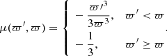
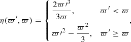
In Paper IV we showed that, in the limit where the number ℒ of layers is infinite, Eqs. (1a) and (1b) can be formally solved regardless of any EOS. In the special case of rigid rotation considered here, we obtain an IDE linking the eccentricity profile ε(a) and the mass density profile ρ(a). In order to render the problem scale-free, the semimajor axis a of a given isopycnic surface is expressed in units of the equatorial radius ϖ = a/R_e ∈ [0, 1], and $\widehat{\rho }=\rho /{\rho }_{\mathrm{c}}$ is the dimensionless mass density (ρ_c is the central mass density). In these conditions, the IDE reads

$$\begin{array}{c}\hfill \frac{\mathrm{d}{\epsilon }^2}{\mathrm{d}\varpi }=\frac{2{\int }_{\widehat{\rho }(0)}^{\widehat{\rho }(\varpi )}\mathrm{d}\widehat{\rho }({\varpi }^{\prime })\chi ({\varpi }^{\prime },\varpi ;\epsilon )}{{\int }_{\widehat{\rho }(0)}^{\widehat{\rho }(1)}\mathrm{d}\widehat{\rho }({\varpi }^{\prime })\mu ({\varpi }^{\prime },\varpi ;\epsilon )},\end{array}$$(3)

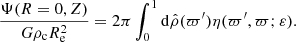
where χ and μ are continuous smooth functions in the whole domain ϖ ∈ [0, 1]. These are defined in Paper IV (see also Appendix A, respectively Eqs. (A.3) and (A.4)). As explicitly stated, χ and μ depend on the radius ϖ and on the eccentricity profile ε(ϖ). We can safely replace Eqs. (1a) and (1b) by Eq. (3), and express Eq. (1a) along the polar axis. This is possible as the gravitational potential is known. As the constant in the RHS, we can take the value of the LHS at the pole, which is the most straightforward. After some algebra (see Appendix C for a proof), we find for the dimensionless enthalpy

$$\begin{array}{c}\hfill \widehat{H}(\varpi )=\widehat{H}(1)+2\pi {\int }_{\widehat{\rho }(0)}^{\widehat{\rho }(1)}\mathrm{d}\widehat{\rho }({\varpi }^{\prime })[\eta ({\varpi }^{\prime },1;\epsilon )-\eta ({\varpi }^{\prime },\varpi ;\epsilon )],\end{array}$$

where $\widehat{H}=H/G{\rho }_{\mathrm{c}}{R}_{\mathrm{e}}^2$, and η is reported in Appendix A (see Eq. (A.5)). It follows that Eq. (1), in the framework of the theory of NSFoE, becomes

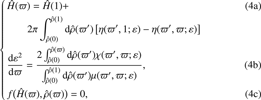
where the last equation is the EOS. We note that, if the mass density profile happens to be known in advance (e.g., deduced from observational data) or prescribed, Eq. (4a) is not needed anymore (see, e.g., Sect. 5.3). We immediately see that the problem is now fully one-dimensional. It means that we can compute the 2D structure of a rotating gaseous body from a 1D approach. This dimension reduction thus relies on a SSB approximation.

2.2. Unfolding and global quantities

Once the 1D solution $\{\widehat{\rho }(\varpi ),\epsilon (\varpi )\}$ is calculated, we can reconstruct any bidimensional map by unfolding the mass density, at each radius a, along the corresponding ellipse E(a, b) up to the polar axis at (0, b), as depicted in Fig. 1. In spherical polar coordinates (r, θ, φ), we actually have

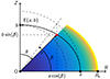Fig. 1. Schematic of the unfolding process. The one-dimensional equation set is first solved for the mass density ρ and eccentricity ε along the equatorial axis in the full interval [0, Re]. Then, the two-dimensional structure is reconstructed by propagating, for each radius (a, 0), the solution (enthalpy, mass density, or pressure) along the ellipse E(a, b) up to the polar axis at (0, b) (see Sect. 2.2).

$$\begin{array}{c}\hfill \widehat{\rho }(r,\theta )=\widehat{\rho }(\varpi ),\end{array}$$(5)

where the two coordinates are easily determined by using the parametric formula

with θ ∈ [0, π/2] and β ∈ [0, π/2], and where

$$\begin{array}{c}\hfill \overline{\epsilon }(\varpi )={[1-{\epsilon }^2(\varpi )]}^{1/2}\end{array}$$(7)

is the axis ratio of the isopycnic E(a, b) considered. The conversion to cylindrical coordinates is straightforward: R = R_eϖcos(β) and $Z=R_{\mathrm{e}}\varpi \overline{\epsilon }(\varpi )sin(\beta )$. We can subsequently deduce all global quantities (e.g., mass, volume).

In (ϖ,β, φ) coordinates, the volume element writes

$$\begin{array}{c}\hfill \frac{\mathrm{d}V}{R_{\mathrm{e}}^3}=2\pi \frac{{\varpi }^{2}cos(\beta )}{\overline{\epsilon }(\varpi )}[{\overline{\epsilon }}^2(\varpi )-\frac{1}{2}{sin}^2(\beta )\frac{\mathrm{d}{\epsilon }^2}{\mathrm{d}\varpi }]\mathrm{d}\varpi \mathrm{d}\beta \mathrm{d}\phi .\end{array}$$(8)

For most global properties of the system, the integrations over β are trivial. For instance, the mass M and the moment of inertia I are reduced to a single integral over ϖ and we have

$$\begin{array}{c}\hfill \{\begin{array}{cc}& \frac{M}{{\rho }_{\mathrm{c}}{R}_{\mathrm{e}}^3}=4\pi {\int }_0^1\mathrm{d}\varpi \frac{{\varpi }^2\widehat{\rho }(\varpi )}{\overline{\epsilon }(\varpi )}[{\overline{\epsilon }}^2(\varpi )-\frac{1}{6}\frac{\mathrm{d}{\epsilon }^2}{\mathrm{d}\varpi }],\hfill \\ \hfill & \frac{I}{{\rho }_{\mathrm{c}}{R}_{\mathrm{e}}^5}=\frac{8}{3}\pi {\int }_0^1\mathrm{d}\varpi \frac{{\varpi }^4\widehat{\rho }(\varpi )}{\overline{\epsilon }(\varpi )}[{\overline{\epsilon }}^2(\varpi )-\frac{1}{10}\frac{\mathrm{d}{\epsilon }^2}{\mathrm{d}\varpi }].\hfill \end{array}\end{array}$$(9)

According to Paper IV, the rotation rate Ω is given by

$$\begin{array}{c}\hfill {\widehat{\mathrm{\Omega }}}^2=-2\pi {\int }_{\widehat{\rho }(0)}^{\widehat{\rho }(1)}\mathrm{d}\widehat{\rho }({\varpi }^{\prime })\kappa ({\varpi }^{\prime },\varpi ;\epsilon ),\end{array}$$(10)

where $\widehat{\mathrm{\Omega }}=\mathrm{\Omega }/\sqrt{G{\rho }_{\mathrm{c}}}$ and κ is defined by Eq. (A.6) (see again Paper IV). It is worth recalling that, as the theory of NSFoE is an approximate theory, Eq. (10) is expected to exhibit slight variations with the radius (see below), and should rigorously be denoted ${\widehat{\mathrm{\Omega }}}^2(\varpi )$.

2.3. Comments

As can be seen in Paper IV, the three functions χ, μ, and η have small amplitude, but all take real, negative values in the range of ϖ of interest. It is therefore clear that, if the integral in Eq. (4a) happens to be essentially negative, then the mass density can become negative, in which case the computed solution cannot be compatible with a physical solution. Density inversions are eventually acceptable, but ρ ≥ 0 is a firm condition. A similar remark holds for Eq. (10). For Eq. (4b), things are less restrictive. Actually, negative values of ε² correspond to prolate spheroids. This is not a problem because there is a mathematical continuity in the gravitational potential when the eccentricity becomes a purely imaginary number (i.e., when ε = 0⁺ → i0⁺; Binney & Tremaine 1987). From a numerical point of view, however, the requires a dedicated treatment, and it seems preferable to consider the axis ratio, namely $\overline{\epsilon }(\varpi )\lessgtr 1$ instead of ε (see below, and Appendix B).

3. Solution with a SCF-algorithm. Implementation and example

3.1. Cycle and convergence criterion

It is well known that Eqs. (1a) and (1b) correspond to a fixed-point problem: ρ = f(ρ) in terms of the mass density profile. Clearly, the equation set Eq. (4) has a similar structure, but we have two coupled fixed-point problems of the form

It is therefore natural to proceed in the same manner as for the standard SCF method: we guess the profiles for the mass density and the axis ratio, namely ${\widehat{\rho }}^{(0)}(\varpi )$ and ${\overline{\epsilon }}^{(0)}(\varpi )$, and let the profiles evolve until stabilization. This can be accomplished following the iterative scheme, for t ≥ 1:

• 1.

  ${\overline{\epsilon }}^{(t)}$ is obtained from Eq. (7), after integrating Eq. (4b);

• 2.

  ${\widehat{H}}^{(t)}$ is computed according to Eq. (4a);

• 3.

  ${\widehat{\rho }}^{(t)}$ is obtained from Eq. (4c).

We see that there are two other options (with no significant impact on the performance of the cycle), depending on the order of assignments; in other words, $\overline{\epsilon }$ in Eq. (11b) can be computed using the ρ-profile updated from Eq. (11a), or ρ in Eq. (11a) can be computed from the $\overline{\epsilon }$-profile updated from Eq. (11b). At convergence, two successive profiles must be numerically unchanged, in which case the cycle ends. As we traditionally use double precision computers, we take^{1, 2}δ^(t) ≲ 10⁻¹⁴, where

$$\begin{array}{c}\hfill {\delta }^{(t)}\equiv max({\mathrm{\Delta }}^{(t)}\widehat{\rho },{\mathrm{\Delta }}^{(t)}\overline{\epsilon }),\end{array}$$(12)

where we define still for t ≥ 1 and ϖ ∈ [0, 1]

$$\begin{array}{c}\hfill {\mathrm{\Delta }}^{(t)}\widehat{\rho }=sup|{\widehat{\rho }}^{(t)}(\varpi )-{\widehat{\rho }}^{(t-1)}(\varpi )|,\end{array}$$(13)

and use a similar definition for ${\mathrm{\Delta }}^{(t)}\overline{\epsilon }$.

3.2. Boundary conditions

In the standard (single-domain) case, and in the absence of external pressure (see Sect. 5.2), we can take Dirichlet boundary conditions (BCs) at the outer boundary ϖ = 1

$$\begin{array}{c}\hfill \{\begin{array}{cc}& \widehat{\rho }(1)=0\hfill \\ \hfill & \overline{\epsilon }(1)={\overline{\epsilon }}_{\mathrm{s}}\hfill \end{array},\end{array}$$(14)

where ${\overline{\epsilon }}_{\mathrm{s}}=R_{\mathrm{p}}/R_{\mathrm{e}}$ is the axis ratio of the outermost surface. At the center of the body, we have

$$\begin{array}{c}\hfill \{\begin{array}{cc}& \widehat{\rho }(0)=1\hfill \\ \hfill & {\frac{\mathrm{d}{\overline{\epsilon }}^2}{\mathrm{d}\varpi }|}_{\varpi =0}=0\hfill \end{array}.\end{array}$$(15)

Unfortunately, $\overline{\epsilon }(0)$ cannot be easily deduced.

3.3. Method and implementation (quadrature schemes, ϖ-grid, and seeds)

We see that Eq. (4) involves derivatives and quadratures, and there are different ways to estimate ρ(ϖ) and $\overline{\epsilon }(\varpi )$ for given BCs. Here we decided to recast Eq. (4b) in integral form, i.e.,

$$\begin{array}{c}\hfill {\overline{\epsilon }}^2(\varpi )={\overline{\epsilon }}_{\mathrm{s}}^2-{\int }_{\varpi }^1\left(\frac{\mathrm{d}{\overline{\epsilon }}^2}{\mathrm{d}\varpi }\right)\mathrm{d}\varpi ,\end{array}$$(16)

where the term in parentheses is simply the right-hand side of Eq. (4b) within a minus sign. So, we have only to deal with quadratures. The eccentricity being unknown at the center, we chose to integrate downward, from the surface to the center, with Eq. (14) as Dirichlet BCs. The computational grid is made of N + 1 equally spaced nodes: ${\varpi }_i\in \{0,\frac{1}{N},\cdots ,{\varpi }_i=\frac{i}{N},\cdots ,1\}$. We used the trapezoidal rule as the quadrature rule, which is second-order in the step size (more efficient schemes can be used at this level). According to Eq. (14), still assuming null ambient pressure, we take

as the starting guess. Initially, we thus have ${\widehat{H}}^{(0)}(0)={\widehat{H}}_{\mathrm{c}}$ at the center, and ${\overline{\epsilon }}^{(0)}(0)=1$. These quadratic profiles seem appropriate for a wide range of configurations, although the solutions generally have a nonzero central eccentricity. Obviously, the BCs must be applied at each step in the cycle.

3.4. A note about the equation of state

The EOS is the fundamental ingredient. Without loss of generality, we consider a polytropic gas where the pressure is a power law of the mass density, which leads to the expression H = K(n + 1)ρ^1/n, where K is a positive constant and the polytropic index n >  0 is finite. In this case the relationship between $\widehat{H}$ and $\widehat{\rho }$ is

$$\begin{array}{c}\hfill \frac{\widehat{H}}{{\widehat{H}}_{\mathrm{c}}}={\widehat{\rho }}^{1/n},\end{array}$$(18)

where ${\widehat{H}}_{\mathrm{c}}=K(n+1)/G{\rho }_{\mathrm{c}}^{1-1/n}{R}_{\mathrm{e}}^2$ (this relation assumes $\widehat{\rho }\ge 0)$. The mass density ${\widehat{\rho }}^{(t)}$ inside the cycle, including the seed, is deduced from the EOS through Eq. (4c).

3.5. Example of cycle convergence

The first example is for ${\overline{\epsilon }}_{\mathrm{s}}=0.9$ and n = 3, and the grid has N + 1 = 257 equally spaced nodes. This configuration corresponds, for instance, to a radiation-pressure-dominated ideal gas or to a white dwarf with fully degenerate extremely relativistic electrons. With this parameter, we are already beyond slow rotators. We ran the code based on the SSB approximation. Figure 2 shows the evolution of $\widehat{\rho }(\varpi )$ and ε²(ϖ) during the cycle, as well as the deviations $\mathrm{\Delta }\widehat{\rho }$ and Δε² from one step to the other. Figure 2f gives the convergence parameter δ^(t) defined by Eq. (12) from the beginning to convergence. We see that δ^(t) decreases exponentially with the step t and the algorithm converges quickly on a solution. Convergence is reached after 70 cycles with the current criterion. After step 20, we already have δ^(t) ∼ 10⁻⁵, which is on the order of the accuracy of the numerical scheme (i.e., 1/N² ∼ 10⁻⁵ with 257 nodes). The next steps are necessary to reach the threshold of 10⁻¹⁴. We show in Fig. 2c the rotation rate computed from Eq. (10). Unsurprisingly, there is a slight variation with the radius, on the order of 10⁻² in relative. This is due to the approximate nature of the theory of NSFoE. The function κ involved when computing Ω² changes sign for most pairs (ϖ′, ϖ), which in some cases results in subtracting two quantities close to each other, thereby amplifying errors. This effect can be reduced by increasing the numerical resolution. Actually, a test with N = 1024 shows a mean value $⟨{\widehat{\mathrm{\Omega }}}^2⟩\approx 1.3014\times {10}^{-2}$ and an amplitude around 10⁻³ in relative, which is more reasonable.

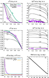Fig. 2. Radial profiles for $\widehat{\rho }$ (panel a) and $\overline{\epsilon }$ (panel b) during the SCF cycle for a few selected steps t (labeled on the curves) of the SCF cycle, and absolute deviations (panels d and e) between steps t − 1 and t. Also shown are the square of the rotation rate (panel c) computed at convergence from Eq. (10) and its mean value (orange), and the convergence parameter δ computed from Eq. (12) as a function of step t (panel f).

We list in Table 1 the main global quantities at equilibrium, namely the mass M, the moment of inertia I, the volume V, the angular momentum J, the gravitational energy W, the kinetic energy T, the internal energy U, and the virial parameter VP = W + 2T + U. We see that VP/|W| is on the order of 10⁻⁴ in absolute, which is very good. We also list the values output by the DROP code, which solves Eq. (1) in full 2D (Huré & Hersant 2017; Basillais & Huré 2021). We see that the agreement between the two methods is quite good, with deviations on the order of a few 10⁻³ in relative, while the resolution is moderate.

3.6. Example of two-dimensional reconstruction (deprojection)

Once a solution in the form of a pair of profiles $\widehat{\rho }(\varpi )$ and ε(ϖ) is known, we can reconstruct the 2D structure by using Eq. (2). For this second example, we ran the SCF code under the same conditions as above, but for ${\overline{\epsilon }}_{\mathrm{s}}=0.75$ and n = 1.5, which could correspond to a fast-rotating fully convective star. We note that ${\overline{\epsilon }}_{\mathrm{s}}\approx 0.74$ for Achernar (Domiciano de Souza et al. 2014). We can compare the ρ-map obtained in this way to the field output by the DROP code. This is shown in Fig. 3. We see that the largest differences are mainly located close to the surface, as the true solution is slightly sub-elliptical. The deviations do not exceed about 3 × 10⁻³ in absolute (this value is on the order of the virial parameter, see below). This result is remarkable, in particular because the surface is the place where the mass density is small and vanishes. The best agreement is observed at the center, at the pole, and at the equator, with absolute deviations of about 10⁻⁵. The main quantities are reported in Table 2. We see that most global quantities are correctly reproduced within a percent, which is satisfying for a rotator this fast.

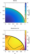Fig. 3. Color-coded mass density map (log. scale) computed from Eq. (4) that takes advantage of dimension reduction (top) and absolute difference (log. scale) with the reference DROP code (bottom), for configuration B. The parameters are ${\overline{\epsilon }}_{\mathrm{s}}=0.75$ and n = 1.5, with 257 nodes per direction (see also Table 2).

3.7. Varying the surface axis ratio and the polytropic index: Computing vs. precision

We performed similar comparisons by varying the surface axis ratio ${\overline{\epsilon }}_{\mathrm{s}}$ and the polytropic index n, again with a moderate numerical resolution corresponding to N = 256. The results are gathered in Table F.1, where we list the mass, the rotation rate, the relative virial parameter and the root mean square (RMS) difference between the two structures (mass, density). There are three series. For the first the index and the resolution are held fixed (n = 1.5, N = 256) and the surface eccentricity increases to the critical rotation, at about ${\overline{\epsilon }}_{\mathrm{s}}\approx 0.62$. In the second series the surface eccentricity and the resolution are fixed (${\overline{\epsilon }}_{\mathrm{s}}=0.95$, N = 256) and n varies from 0.5 to 4. In the last series, the configuration is fixed (${\overline{\epsilon }}_{\mathrm{s}}=0.95$, n = 1.5) and we increase the resolution from 32 to 2048. We see that the agreement is good: the maximum RMS value is 4 × 10⁻³ and the mass and rotation rate are well reproduced within a percent. From the virial parameters and the RMS, two trends are seen. First, the method is less and less accurate as the axis ratio decreases, especially for a “hard” EOS. This is expected because the true surface deviates more from a perfect spheroid as the rotation becomes faster. Second, the method is increasingly accurate as the polytropic index increases (“soft” EOS), even close to critical rotations. As n increases, the density becomes peaked at the center, and the contribution to the mass (and potential) of the “wings” becomes small to negligible. This is visible in Fig. 2a, for instance. For n = 3 the mass density vanishes quickly toward the surface ($\widehat{\rho }\lesssim {10}^{-3}$ at ϖ ≳ 0.7).

The computing time reported in the table is obtained on a standard laptop, without any specification optimization. For n = 1.5 and ${\overline{\epsilon }}_{\mathrm{s}}=0.95$, the number of iterations is about 30 and is not sensitive to N. We find ∼(N/581.295)^1.930 s for convergence with the SSB approximation, to be compared to the full 2D problem ∼(N/77.824)^3.089 s.

4. More tests

In order to better see the power of the method and its flexibility, we present in this section several tests, including static and rotating configurations (see next section for systems with mass density jumps). The convergence criterion and the numerical resolution are (unless stated otherwise) the same as in Sect. 3.5.

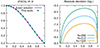Fig. 4. Mass density profile obtained by solving Eq. (4) with the SCF algorithm (N = 256) in the static case (${\overline{\epsilon }}_{\mathrm{s}}=1)$ and for n = 1, compared to the corresponding exact solution of the Lane-Emden equation (left panel). Also shown is the absolute deviation between these two solutions, for several values of N (right panel); see also Table 3.

4.1. Static case with index unity

We consider here a static gas with polytropic index n = 1 (see Sect. 1). All isobars are spherical and ε = 0 for any ϖ. In this case the solution of the Lane-Emden equation is analytical³, namely

$$\begin{array}{c}\hfill \widehat{\rho }(\varpi )=\frac{sin(\pi \varpi )}{\pi \varpi },\end{array}$$(19)

which enables a direct comparison. The theory of NSFoE is exact for spherical configuration because the confocal parameters are null, which is therefore the case of Eq. (4). If we inject ε(ϖ)=0 in the four functions κ, χ, μ, and η, an expansion is required in the limit ε → 0. We find that ε = 0 is in fact a regular singular point, and it follows that κ = χ = 0 (see Appendix D). Thus, we recover that the body is nonrotating and that all isopycnics are spherical. We have applied the SSB approximation. The results are shown in Fig. 4. The main output data are listed in Table 3. We see that the deviation from the analytical solution is of order 10⁻⁵, and it decreases as N increases. This occurs because deviations are directly linked to the order of the quadrature scheme in this case.

4.2. The case of slow rotation

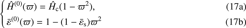
In the limit of slow rotation, various approximations can be found (see, e.g., Chandrasekhar 1933). Of particular interest is Clairaut’s theory, which is first-order accurate in the square of the eccentricity, ε² ≪ 1. It happens that there are a few closed-form solutions to Clairaut’s second-order differential equation compatible with physically realistic BCs. Among them, Tisserand (1891) and Marchenko (2000) have a Legendre-Laplace solution for n = 1: the solution is the same as for the nonrotating case (i.e., a sine cardinal for the mass density)⁴. For Eq. (19), the eccentricity profile reads

$$\begin{array}{c}\hfill {\overline{\epsilon }}^2(\varpi )=1-(1-{\overline{\epsilon }}_{\mathrm{s}}^2)\frac{({\pi }^2{\varpi }^2-3)sin(\pi \varpi )+3\pi \varpi cos(\pi \varpi )}{3{\varpi }^2[\pi \varpi cos(\pi \varpi )-sin(\pi \varpi )]}.\end{array}$$(20)

We ran the code for n = 1 and ${\overline{\epsilon }}_{\mathrm{s}}=0.99$. The results are displayed in Fig. 5. We see that the mass density profile of the rotating case departs only slightly from a sine cardinal (the deviation is of order 10⁻³). More importantly, the actual method yields an eccentricity profile that is very close to Eq. (20), within a few 10⁻⁵ in absolute, which is highly satisfying. This confirms the efficiency of the SSB approximation at slow rotation. Figure 6 displays the mass density structure and the deviation from the reference structure, with a RMS value of 2 × 10⁻⁶.

Fig. 5. Mass density profile and squared eccentricity profile (left panels) obtained by solving Eq. (4) with the SCF algorithm, and comparison with the exact nonrotating first-order solution from Clairaut’s fundamental equation (right panels).

Fig. 6. Same as Fig. 3, but for ${\overline{\epsilon }}_{\mathrm{s}}=0.99$ and n = 1.

4.3. A case of moderate rotation

An interesting test concerns the transition from slow to moderate rotators. We performed a new run for n = 1 and ${\overline{\epsilon }}_{\mathrm{s}}=0.95$ (which is close to the axis ratio of Jupiter, for instance). The results are shown in Fig. 7 after reconstruction of the 2D map for the mass density. We see that the deviation is again maximum at the surface, midway between the pole and the equator. The highest value of the RMS for the mass density is about 3 × 10⁻⁴, while the mean value is about 7 × 10⁻⁵. At the center, near the pole and the equator, the precision is excellent, with more than six correct digits.

Fig. 7. Same as Fig. 3, but for ${\overline{\epsilon }}_{\mathrm{s}}=0.95$ and n = 1.

4.4. Reproduction of Hachisu’s (j², ω²) sequences of equilibrium

In the 1980s Hachisu and collaborators perfomed a wide exploration of figures of equilibrium through a series of fundamental papers (Hachisu 1986a, 1986b). They computed sequences of axially symmetrical equilibria by varying the surface axis ratio ${\overline{\epsilon }}_{\mathrm{s}}$, both for stars and rings (out of range here). The configurations are gathered in the (j², ω²)-plane, where ω and j are the normalized rotation rate Ω and angular momentum J, respectively, defined as

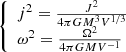$$\begin{array}{c}\hfill \{\begin{array}{c}{j}^2=\frac{J^2}{4\pi G{M}^3{V}^{1/3}}\hfill \\ {\omega }^2=\frac{{\mathrm{\Omega }}^2}{4\pi GM{V}^{-1}}\hfill \end{array}\end{array}$$(21)

Hachisu (1986a) showed that, in contrast to the Maclaurin uncompressible sequence, all sequences are open, depending on the polytropic index n >  0 of the gas: the larger the value of n, the larger the gap. Figure 8 shows a few points of the sequences obtained with the SSB approximation for n = {0.1, 0.5, 1.5, 3, 4}, together with the data extracted from Hachisu’s paper (same axis ratio). Values obtained in full 2D with the DROP code are also plotted for comparison. We see that the agreement is excellent, except for points close to critical rotations. This is obviously due to the deviation of the external surface to a spheroid: the volume is overestimated in this case, which causes a double shift in the diagram, toward higher ω-values and lower j-values. The best results are obtained for weakly compressible gas. The virial parameters, on the other hand, are better and better as n increases (see Sect. 3.6).

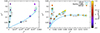Fig. 8. The (j2, ω2) diagram for several polytropic indices n labeled on the curves. The solid lines correspond to the solutions obtained from DROP code. The empty circles are the solutions reported in the tables of Hachisu (1986a). The full circles are the solutions obtained with the SCF method with dimension reduction. The color-coding indicates the decimal logarithm of the relative virial parameter |VP/W|.

5. Cases with mass density jumps

5.1. Changes

Bodies made of different inhomogeneous domains separated by mass density jumps are of immense interest. Such cases are studied in Paper IV. We now consider 𝒦 domains where the mass density ρ_k(ϖ) varies (domain no. 1 is for the innermost domain and k = 𝒦 is for the outermost one). Then we can write the full mass density profile from the center to the surface as

$$\begin{array}{c}\hfill \widehat{\rho }(\varpi )=\sum _{k=1}^{\mathcal{K}}[{\widehat{\rho }}_k(\varpi )-{\widehat{\rho }}_{k+1}(\varpi )]\mathcal{H}({\varpi }_k-\varpi ),\end{array}$$(22)

where ϖ_k is the position, along the equatorial axis, of the mass density jump between domains k and k + 1, and ℋ is Heaviside’s distribution. For convenience we set ρ_𝒦 + 1 = 0 to keep a single sum in Eq. (22). The radial derivative is then given by the expression

$$\begin{array}{cc}\hfill \frac{\mathrm{d}\widehat{\rho }}{\mathrm{d}\varpi }& =\sum _{k=1}^{\mathcal{K}}[\frac{\mathrm{d}{\widehat{\rho }}_k}{\mathrm{d}\varpi }-\frac{\mathrm{d}{\widehat{\rho }}_{k+1}}{\mathrm{d}\varpi }]\mathcal{H}({\varpi }_k-\varpi )\hfill \\ \hfill & -\sum _{k=1}^{\mathcal{K}}[{\widehat{\rho }}_k(\varpi )-{\widehat{\rho }}_{k+1}(\varpi )]\delta ({\varpi }_k-\varpi ),\hfill \end{array}$$(23)

where δ is Dirac’s distribution. So, for any continuous function f(ϖ′,ϖ) in the interval [0, 1]², we have

$$\begin{array}{cc}\hfill {\int }_{\widehat{\rho }(0)}^{\widehat{\rho }(1)}\mathrm{d}\widehat{\rho }({\varpi }^{\prime })f({\varpi }^{\prime },\varpi )& =\sum _{k=1}^{\mathcal{K}}{\int }_{{\widehat{\rho }}_k({\varpi }_{k-1})}^{{\widehat{\rho }}_k({\varpi }_k)}\mathrm{d}{\widehat{\rho }}_k({\varpi }^{\prime })f({\varpi }^{\prime },\varpi )\hfill \\ \hfill & -\sum _{k=1}^{\mathcal{K}}\frac{{\alpha }_k-1}{{\alpha }_k}{\widehat{\rho }}_k({\varpi }_k)f({\varpi }_k,\varpi ),\hfill \end{array}$$(24)

where ϖ₀ = 0 again for convenience, and the mass density jump α_k is defined by

$$\begin{array}{c}\hfill {\alpha }_k=\frac{{\rho }_k({\varpi }_k)}{{\rho }_{k+1}({\varpi }_k)}.\end{array}$$(25)

It follows that the structure of a rigidly rotating body made of several inhomogeneous domains can be treated with dimension reduction by solving Eqs. (4a) and (4b), where all the integrals are estimated from Eq. (24).

5.2. Presence of an ambient pressure

As the present formalism relies mainly on a barotropic EOS, we assume the external pressure to be constant along the outermost surface of the object: P_amb. Thus, this value corresponds to a cutoff for the mass density at ${\widehat{\rho }}_{\mathrm{amb}}$, and then to a mass density jump at ϖ = 1. In the case of a single domain object (𝒦 = 1 and ϖ₁ = 1 here), we have

$$\begin{array}{c}\hfill \widehat{\rho }(\varpi )={\widehat{\rho }}_1(\varpi )\mathcal{H}(1-\varpi ),\end{array}$$(26)

where ${\widehat{\rho }}_1(1)={\widehat{\rho }}_{\mathrm{amb}}$. An interesting test case for ambient pressure is the n = 5 polytrope. The analytical solution in the nonrotating case is due to Schuster (e.g., Horedt 2004; see note 3). In the present context, the solution must be truncated at the right isobar P(1)=P_amb. The analytical solution becomes

$$\begin{array}{c}\hfill \widehat{\rho }(\varpi )=\frac{1}{{[1+{\varpi }^2({\widehat{\rho }}_{\mathrm{amb}}^{-2/5}-1)]}^{5/2}},\end{array}$$(27)

which verifies $\widehat{\rho }(0)=1$ and $\widehat{\rho }(1)={\widehat{\rho }}_{\mathrm{amb}}$. We computed the solution from the SSB approximation. We note that the method is not appropriate for the case ${\widehat{\rho }}_{\mathrm{amb}}=0$ because the mass and especially the radius are infinite for P_amb = 0. The reconstructed mass density map is displayed in Fig. 9, and the main data are listed in Table 4. As for the n = 1 static case, we see that the agreement is excellent and the deviation from the exact solution depends just on the resolution, as expected. We note that the virial parameter was adapted to the context of an ambient pressure. We have

$$\begin{array}{c}\hfill \mathrm{VP}=W+2T+U-U_{\mathrm{amb}},\end{array}$$(28)

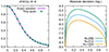Fig. 9. Mass density profile obtained by solving Eq. (4b) with the SCF algorithm and N = 256, with configuration ${\overline{\epsilon }}_{\mathrm{s}}=1$, n = 5, and ${\widehat{\rho }}_{\mathrm{amb}}=0.04$ (configuration C), compared to the exact solution of Schuster (left panel), and the absolute deviation between these two solutions for several values of N (right panel).

where U_amb = 3P_ambV (see, e.g., Cox & Giuli 1968).

5.3. The Earth as a an example

Dziewonski & Anderson (1981) obtained a seismologic model for the internal structure of the Earth, named the Preliminary Reference Earth Model (PREM). They derived profiles for the mass density, pressure, and gravitational field of the Earth under the hypothesis of a purely spherical planet. In this section we use the mass density profile of the PREM as an input to model a rotating Earth with the SSB approximation; it is plotted in Fig. 11a. It is clear that nonspherical effects have an impact on the mass density distribution. However, the Earth is a slow rotator, so the deviation is expected to be on the order of $1-{\overline{\epsilon }}_{\mathrm{s}}\sim 3\times {10}^{-3}$ in relative. The PREM is a model with 𝒦 = 10 domains, and as many mass density jumps⁶. As $\widehat{\rho }(\varpi )$ is an input, the SSB approximation developed in this work returns to a single fixed-point problem where only step (i) of the cycle is needed (i.e., we iterate only on Eq. (4b)). Only 15 iterations are required by the SCF method (with N = 1024 per domain). We show the results for dε²/dϖ and ε²(ϖ) in Figs. 11b and c, respectively. We also report the eccentricity profile computed by Ragazzo (2020), who solved Clairaut’s equation with the same piece-wise prescription for the mass density. We see that both solutions are in excellent agreement. The pressure profile P(ϖ) at equilibrium is visible in Fig. 11d (see Appendix E for this calculation). It compares very well to the PREM values (the central dimensionless value is ∼0.782 comparted to 0.784 for the PREM). The relative deviations do not exceed ∼3 × 10⁻³, which is on the order of the flattening of the outermost surface. This departure is not due to the spheroidal approximation made in this work (as |VP/W|∼7 × 10⁻⁷), but to the fact that the observed mass density profile has been spherically averaged by the PREM and that centrifugal effects have not been taken into account in their calculations of the pressure profile.

Fig. 11. Main outputs for the Earth using the PREM. From left to right: normalized mass density of the PREM (Dziewonski & Anderson 1981) which is used as an input in this work, and the gradient of the eccentricity squared, squared eccentricity, and normalized pressure determined from the SSB approximation.

In the rotating case, Schuster’s solution is not adapted anymore, and we switch back to the DROP code for the reference. For this illustration we consider the configuration given in Table 5. It is an intermediate rotator with the same index and ambient pressure as before. A comparison between the full 2D solution and the reconstructed density field, as well as the difference between the two maps, is shown in Fig. 10. We see that the RMS error⁵ is on the order of 10⁻⁴. The main global quantities are given in Table 5. The agreement is once again very good, with local deviations on the order of 10⁻⁴ on the density profile. For global properties, the relative deviations are on the order of 10⁻³.

Fig. 10. Same as Fig. 3, but for ${\overline{\epsilon }}_{\mathrm{s}}=0.90$, n = 5.0, and ${\widehat{\rho }}_{\mathrm{amb}}=0.04$ (configuration C); see also Table 5.

The global properties deduced from SSB approximation are reported in Table 6. However, the data in this table must be rescaled prior to any comparison with observational data. For this purpose we chose to use the mass and equatorial radius given by Chambat et al. (2010), and reported in Table 7. We then deduced ρ_c = 13 083.8 kg m⁻³, whose value remains close to the PREM value of 1.3088 × 10⁴ kg m⁻³. Table 7 compares the momentum of inertia, rotation rate, and first two gravitational moments. We see that the normalized moment of inertia and the rotation rates are in good agreement with the observational data, again within ∼3 × 10⁻³ in relative. Regarding the gravitational moments, we see that J₂ is close to the observed value, roughly within 1%. The result is worse for J₄, a deviation reaching 75%. A similar discrepancy is found by Chambat et al. (2010), who solved the second-order Clairaut’s equation with a different (yet similar) mass density profile for the Earth. As quoted by these authors, this deviation from the observed gravitational moments is due to nonhydrostatic characteristics of the Earth, which are not taken into account in our equation set.

6. Summary

In this article we showed that the 2D structure of a rotating self-gravitating fluid can be determined with good precision from the theory of Nested Spheroidal Figures of Equilibrium, which assumes that isopycnics are perfect spheroids. The method uses the general IDE established in Staelen & Huré (2024), connecting the local eccentricity ε of isopynics to the local mass density ρ. As this equation involves only the equatorial radius, it can be coupled to the centrifugal balance along the polar axis, providing a specific one-dimensional projection of the genuine bi-dimensional problem. As shown, the new problem consists in solving two fixed-points problems coupled together. From the equatorial solution {ρ(a),ε(a)}, which can be determined by a simple SCF method, we recover the full structure by propagating the mass density along the ellipse, from the equator to the pole, and for any equatorial radius a ∈ [0, R_e]. We provided a series of examples supporting the efficiency and versatility of this SSB approximation. In particular, the method is well suited to systems made of heterogeneous domains separated by mass density jumps. It can account for an ambient pressure. The method is also flexible in terms of barotropic EOS. Here we used a polytrope, but any kind of P(ρ)-relation is usable. The main results of this paper can be summarized as follows:

• The SSB approximation is exact for nonrotating gas, because the NSFoE is also exact in this case (all confocal parameters are null). The method is then equivalent to a standard Lane-Emden solver. The precision is then fully governed by the numerical schemes implemented.

• For slow rotators (i.e., small flattenings), the method has an excellent precision. Depending on the EOS, the solution can reproduce the full 2D mass density profile, typically within 10⁻⁵ in absolute (dimensionless profile), even at low to moderate numerical resolution.

• For fast rotators (i.e., large flattenings), the SSB approximation furnishes good and reliable results, whatever the EOS.

• For hard EOSs (typically 0 <  n <  1), the deviation of the true surface from a spheroid is very small, but there is a significant amount of matter close to the surface. The precision of SSB approximation is very good provided the system stays far from the critical rotation state. Near the sequence endings, the precision is acceptable, with typically 1% in the mass density (RMS value).

• For soft EOSs (n >  1) the precision is very good because the amount of matter located close to the surface has a negligible contribution to the total mass (and gravitational potential), although the deviation of the true surface from a spheroid is significant.

• Compared to the full 2D problem in which the surface and isoycnics are not constrained, the mass density in the vicinity of the center computed with the SSB approximation has an excellent precision. This is also true for values close to the pole and to the equator.

• The computing time is reduced by at least two orders of magnitude with respect to the full 2D problem. This is a direct consequence of dimension reduction. This enables us to reach very high numerical resolutions in a short time, which is particularly attractive for generating grids of models for instance.

Acknowledgments

We are grateful to F. Chambat for informed comments on the paper before submission. We thank the anonymous referee for suggestions to improve the paper and valuable references, in particular on the state-of-art regarding stellar models.

References

Appendix A: The functions χ, μ, ν, and η

We define for convenience

$$\begin{array}{c}\hfill e^2(c)=\frac{\varpi {\prime }^2{\epsilon }^2({\varpi }^{\prime })}{{\varpi }^2[1+c]},\end{array}$$(A.1)

and $\overline{e}(c)=\sqrt{1-e^2(c)}\ge 0$, where the continuous confocal parameter c ≡ c(ϖ′,ϖ) is given by

$$\begin{array}{c}\hfill c({\varpi }^{\prime },\varpi )=\frac{\varpi {\prime }^2{\epsilon }^2({\varpi }^{\prime })}{{\varpi }^2}-{\epsilon }^2(\varpi ).\end{array}$$(A.2)

In these conditions, and given the function $\mathcal{A}(\overline{\epsilon })$ defined by Eq.(B.1), χ is defined as

$$\begin{array}{c}\hfill \chi ({\varpi }^{\prime },\varpi ;\epsilon )=\{\begin{array}{ccc}& \frac{\varpi {\prime }^3\overline{\epsilon }({\varpi }^{\prime })}{{\varpi }^4}[\mathcal{A}(\overline{e}(0))-\frac{\mathcal{A}(\overline{e}(c))}{\sqrt{1+c}}],\hfill & \hfill {\varpi }^{\prime }<\varpi \\ \hfill & 0,\hfill & \hfill {\varpi }^{\prime }\ge \varpi \end{array},\end{array}$$(A.3)

μ is defined as

$$\begin{array}{c}\hfill \mu ({\varpi }^{\prime },\varpi ;\epsilon )=\{\begin{array}{ccc}& \frac{{\varpi }^{\prime }\overline{\epsilon }({\varpi }^{\prime })\mathcal{A}(\overline{e}(c))}{\varpi {\epsilon }^2({\varpi }^{\prime })\sqrt{1+c}}-\frac{{\varpi }^{\prime }\overline{\epsilon }({\varpi }^{\prime })}{\varpi {\epsilon }^2({\varpi }^{\prime })\overline{\epsilon }(\varpi )},\hfill & \hfill {\varpi }^{\prime }<\varpi \\ \hfill & \frac{\overline{\epsilon }({\varpi }^{\prime })}{{\epsilon }^2({\varpi }^{\prime })}\mathcal{A}(\overline{\epsilon }({\varpi }^{\prime }))-\frac{1}{{\epsilon }^2({\varpi }^{\prime })},\hfill & \hfill {\varpi }^{\prime }\ge \varpi \end{array},\end{array}$$(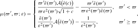A.4)

η is defined as

$$\begin{array}{c}\hfill \eta ({\varpi }^{\prime },\varpi ;\epsilon )=\{\begin{array}{ccc}& {\varpi }^{\prime }\varpi \frac{\overline{\epsilon }({\varpi }^{\prime })}{{\epsilon }^2({\varpi }^{\prime })}[\mathcal{A}(\overline{e}(c))\sqrt{1+c}-\overline{\epsilon }(\varpi )]\hfill & \hfill {\varpi }^{\prime }<\varpi \\ \hfill & {\varpi }^2[1+c]\frac{\overline{\epsilon }({\varpi }^{\prime })}{{\epsilon }^2({\varpi }^{\prime })}\mathcal{A}(\overline{\epsilon }({\varpi }^{\prime }))-{\varpi }^2\frac{{\overline{\epsilon }}^2(\varpi )}{{\epsilon }^2({\varpi }^{\prime })},\hfill & \hfill {\varpi }^{\prime }\ge \varpi \end{array},\end{array}$$(A.5)

and κ is defined as

$$\begin{array}{c}\hfill \kappa ({\varpi }^{\prime },\varpi ;\epsilon )=\{\begin{array}{ccc}& \frac{{\varpi }^{\prime }\overline{\epsilon }({\varpi }^{\prime })}{\varpi {\epsilon }^2({\varpi }^{\prime })}\{[1-2e^2(0)]\mathcal{A}(\overline{e}(0))-2\overline{\epsilon }(\varpi )-\overline{e}(0)+2\mathcal{A}(\overline{e}(c))\sqrt{1+c}\},\hfill & \hfill {\varpi }^{\prime }<\varpi \\ \hfill & \frac{3-2{\epsilon }^2(\varpi )}{{\epsilon }^2({\varpi }^{\prime })}[\overline{\epsilon }({\varpi }^{\prime })\mathcal{A}(\overline{\epsilon }({\varpi }^{\prime }))-1]+1,\hfill & \hfill {\varpi }^{\prime }\ge \varpi \end{array}.\end{array}$$(A.6)

Appendix B: A single function for the prolate and oblate cases

As can be seen in Paper IV, which is devoted to oblate configurations, all functions κ, χ, μ, (and η) depend on ε, which appears in the argument of an arcsin function. During the numerical tests, we dealth with transition states where the deep isopycnic surfaces are slightly prolate, resulting in a purely imaginary eccentricity. This naturally creates numerical issues, which can be circumvented by a simple prolongation since arcsin(z)=arcsinh(iz)/i, where i is the imaginary unit and z is a complex number (see, e.g., Gradshteyn & Ryzhik 2014). So, for the numerical computation we define

$$\begin{array}{c}\hfill \mathcal{A}(\overline{\epsilon })=\{\begin{array}{ccc}& \frac{arcsin(\sqrt{1-{\overline{\epsilon }}^2})}{\sqrt{1-{\overline{\epsilon }}^2}},\hfill & \hfill 0<\overline{\epsilon }<1,\\ \hfill & 1,\hfill & \hfill \overline{\epsilon }=1,\\ \hfill & \frac{\mathrm{arcsinh}(\sqrt{{\overline{\epsilon }}^2-1})}{\sqrt{{\overline{\epsilon }}^2-1}},\hfill & \hfill \overline{\epsilon }>1,\end{array}\end{array}$$(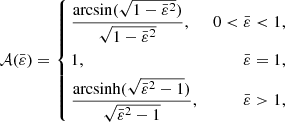B.1)

which enables us to make the transition from oblate to prolate configurations. It can be verified (see Appendix A), by introducing this function 𝒜 in all integrand kernels defined in Paper IV, that only real terms like $\overline{\epsilon }$ or ε² finally survive, whatever the case, either oblate or prolate.

Appendix C: The enthalpy profile

Along the polar axis R = 0, the Bernoulli equation Eq. (1a) reads

$$\begin{array}{c}\hfill H(0,Z)+\mathrm{\Psi }(0,Z)=C^{\mathrm{te}}.\end{array}$$(C.1)

In order to estimate Ψ(0, Z), we need to go back to Paper II. The gravitational potential of a heterogeneous system made of ℒ homogeneous spheroidal layers is given in that article by Eq. (14). At point A_j, at the intersection between the polar axis and the interface between layers j and j + 1, it reads

$$\begin{array}{cc}\hfill \frac{{\mathrm{\Psi }|}_{{\mathrm{A}}_j}}{-2\pi G{a}_j^2}=& \sum _{i=1}^j({\rho }_i-{\rho }_{i+1})\frac{{\overline{\epsilon }}_i}{{\epsilon }_i^3}[(1+c_{i,j})arcsin\left(\frac{q_{i,j}{\epsilon }_i}{\sqrt{1+c_{i,j}}}\right)-q_{i,j}{\epsilon }_i{\overline{\epsilon }}_j]\hfill \\ \hfill & +\sum _{i=1}^j({\rho }_i-{\rho }_{i+1})\frac{{\overline{\epsilon }}_i}{{\epsilon }_i^3}[(1+c_{i,j})arcsin\left({\epsilon }_i\right)(q_{i,j}^2{\epsilon }_i^2+{\overline{\epsilon }}_j^2)-\frac{{\epsilon }_i{\overline{\epsilon }}_j^2}{{\overline{\epsilon }}_i^2}],\hfill \end{array}$$(C.2)

where a_j is the equatorial radius of layer j, ε_j is its eccentricity, ρ_j is its mass density, ${\overline{\epsilon }}_j=\sqrt{1-{\epsilon }_j^2}$, q_i, j = a_i/a_j, and 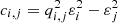$c_{i,j}=q_{i,j}^2{\epsilon }_i^2-{\epsilon }_j^2$. Oblate spheroids were assumed in Paper II, but it can be generalized to any spheroid by introducing the function 𝒜 defined in Appendix B. In the continuous limit ℒ → ∞, we have

$$\begin{array}{c}\hfill \frac{\mathrm{\Psi }(R=0,Z)}{G{\rho }_{\mathrm{c}}{R}_{\mathrm{e}}^2}=2\pi {\int }_0^1\mathrm{d}\widehat{\rho }({\varpi }^{\prime })\eta ({\varpi }^{\prime },\varpi ;\epsilon ).\end{array}$$(C.3)

As H(0, Z) is a function of ϖ only, we define $\widehat{H}(\varpi )=H(0,Z)/(G{\rho }_{\mathrm{c}}{R}_{\mathrm{e}}^2)$. By Eq.(C.1), we have

$$\begin{array}{c}\hfill \widehat{H}(\varpi )+2\pi {\int }_0^1\mathrm{d}\widehat{\rho }({\varpi }^{\prime })\eta ({\varpi }^{\prime },\varpi ;\epsilon )=\widehat{H}(1)+2\pi {\int }_0^1\mathrm{d}\widehat{\rho }({\varpi }^{\prime })\eta ({\varpi }^{\prime },1;\epsilon ),\end{array}$$(C.4)

where the constant C^te was evaluated at the pole of the whole object (i.e., at ϖ = 1). We then see that Eq. (C.4) thus yields Eq. (4a).

Appendix D: The spherical limit

For ε² ≪ 1, we have

$$\begin{array}{c}\hfill \mathcal{A}(\overline{\epsilon })\approx 1+\frac{{\epsilon }^2}{6}\end{array}$$(D.1)

for both $\overline{\epsilon }<1$ and $\overline{\epsilon }>1$. So we can expand functions κ, χ, μ, and η at zeroth order to obtain these functions at $\overline{\epsilon }=1$ (i.e., in the nonrotating spherical case). We have κ(ϖ′,ϖ) = 0, which naturally imposes ${\widehat{\mathrm{\Omega }}}^2=0$ (see Eq. (10)), which means that the body is nonrotating, as expected. Regarding the functions χ and μ appearing in the expression for dε²/dϖ, we have χ(ϖ′,ϖ) = 0 and

$$\begin{array}{c}\hfill \mu ({\varpi }^{\prime },\varpi )=\{\begin{array}{ccc}& -\frac{\varpi {\prime }^3}{3{\varpi }^3},\hfill & \hfill {\varpi }^{\prime }<\varpi \\ \hfill & -\frac{1}{3},\hfill & \hfill {\varpi }^{\prime }\ge \varpi \end{array}.\end{array}$$(D.2)

This thus imposes dε²/dϖ=0 with BC ε²(1)=0. We then recover ε²(ϖ)=0 (i.e., all isopycnic surfaces are spherical, as expected). Finally, the function η needed to compute the enthalpy field becomes

$$\begin{array}{c}\hfill \eta ({\varpi }^{\prime },\varpi )=\{\begin{array}{ccc}& \frac{2\varpi {\prime }^3}{3\varpi },\hfill & \hfill {\varpi }^{\prime }<\varpi \\ \hfill & \varpi {\prime }^2-\frac{{\varpi }^2}{3},\hfill & \hfill {\varpi }^{\prime }\ge \varpi \end{array},\end{array}$$(D.3)

Appendix E: Pressure from the enthalpy field

For any isentropic barotrope, the enthalpy and the pressure are related by

$$\begin{array}{c}\hfill \mathrm{d}\widehat{H}=\mathrm{d}\widehat{P}/\widehat{\rho },\end{array}$$(E.1)

where $\widehat{P}=P/(G{\rho }_{\mathrm{c}}^2{R}_{\mathrm{e}}^2)$ is the dimensionless pressure. So, the pressure profile is given by

$$\begin{array}{c}\hfill \widehat{P}(\varpi )=\widehat{P}(1)-{\int }_{\varpi }^1\mathrm{d}{\varpi }^{\prime }\widehat{\rho }({\varpi }^{\prime })\frac{\mathrm{d}\widehat{H}}{\mathrm{d}{\varpi }^{\prime }}.\end{array}$$(E.2)

We can compute the enthalpy gradient from Eq.(4a). We can show that

$$\begin{array}{c}\hfill \frac{\mathrm{d}\widehat{H}}{\mathrm{d}\varpi }=-2\pi [2\varpi {\overline{\epsilon }}^2(\varpi )-{\varpi }^2\frac{\mathrm{d}{\epsilon }^2}{\mathrm{d}{\varpi }^2}]{\int }_{\widehat{\rho }(0)}^{\widehat{\rho }(1)}\mathrm{d}\widehat{\rho }({\varpi }^{\prime })\mu ({\varpi }^{\prime },\varpi ).\end{array}$$(E.3)

Appendix F: Varying the surface axis ratio and the polytropic index: Computing versus precision

All Tables

All Figures

Fig. 1. Schematic of the unfolding process. The one-dimensional equation set is first solved for the mass density ρ and eccentricity ε along the equatorial axis in the full interval [0, Re]. Then, the two-dimensional structure is reconstructed by propagating, for each radius (a, 0), the solution (enthalpy, mass density, or pressure) along the ellipse E(a, b) up to the polar axis at (0, b) (see Sect. 2.2).

In the text

Fig. 2. Radial profiles for $\widehat{\rho }$ (panel a) and $\overline{\epsilon }$ (panel b) during the SCF cycle for a few selected steps t (labeled on the curves) of the SCF cycle, and absolute deviations (panels d and e) between steps t − 1 and t. Also shown are the square of the rotation rate (panel c) computed at convergence from Eq. (10) and its mean value (orange), and the convergence parameter δ computed from Eq. (12) as a function of step t (panel f).

In the text

	Fig. 3. Color-coded mass density map (log. scale) computed from Eq. (4) that takes advantage of dimension reduction (top) and absolute difference (log. scale) with the reference DROP code (bottom), for configuration B. The parameters are ${\overline{\epsilon }}_{\mathrm{s}}=0.75$ and n = 1.5, with 257 nodes per direction (see also Table 2).
In the text

	Fig. 4. Mass density profile obtained by solving Eq. (4) with the SCF algorithm (N = 256) in the static case (${\overline{\epsilon }}_{\mathrm{s}}=1)$ and for n = 1, compared to the corresponding exact solution of the Lane-Emden equation (left panel). Also shown is the absolute deviation between these two solutions, for several values of N (right panel); see also Table 3.
In the text

	Fig. 5. Mass density profile and squared eccentricity profile (left panels) obtained by solving Eq. (4) with the SCF algorithm, and comparison with the exact nonrotating first-order solution from Clairaut’s fundamental equation (right panels).
In the text

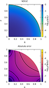	Fig. 6. Same as Fig. 3, but for ${\overline{\epsilon }}_{\mathrm{s}}=0.99$ and n = 1.
In the text

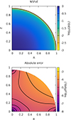	Fig. 7. Same as Fig. 3, but for ${\overline{\epsilon }}_{\mathrm{s}}=0.95$ and n = 1.
In the text

Fig. 8. The (j2, ω2) diagram for several polytropic indices n labeled on the curves. The solid lines correspond to the solutions obtained from DROP code. The empty circles are the solutions reported in the tables of Hachisu (1986a). The full circles are the solutions obtained with the SCF method with dimension reduction. The color-coding indicates the decimal logarithm of the relative virial parameter |VP/W|.

In the text

	Fig. 9. Mass density profile obtained by solving Eq. (4b) with the SCF algorithm and N = 256, with configuration ${\overline{\epsilon }}_{\mathrm{s}}=1$, n = 5, and ${\widehat{\rho }}_{\mathrm{amb}}=0.04$ (configuration C), compared to the exact solution of Schuster (left panel), and the absolute deviation between these two solutions for several values of N (right panel).
In the text

	Fig. 11. Main outputs for the Earth using the PREM. From left to right: normalized mass density of the PREM (Dziewonski & Anderson 1981) which is used as an input in this work, and the gradient of the eccentricity squared, squared eccentricity, and normalized pressure determined from the SSB approximation.
In the text

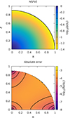	Fig. 10. Same as Fig. 3, but for ${\overline{\epsilon }}_{\mathrm{s}}=0.90$, n = 5.0, and ${\widehat{\rho }}_{\mathrm{amb}}=0.04$ (configuration C); see also Table 5.
In the text

References

- Abramyan, M. G., & Kaplan, S. A. 1974, Astrophysics, 10, 358 [Google Scholar]
- Amendt, P., Lanza, A., & Abramowicz, M. A. 1989, ApJ, 343, 437 [NASA ADS] [CrossRef] [Google Scholar]
- Basillais, B., & Huré, J.-M. 2021, MNRAS, 506, 3773 [NASA ADS] [CrossRef] [Google Scholar]
- Binney, J., & Tremaine, S. 1987, Galactic dynamics (Princeton: Princeton University Press), 747 [Google Scholar]
- Chambat, F., Ricard, Y., & Valette, B. 2010, Geophys. J. Int., 183, 727 [NASA ADS] [CrossRef] [Google Scholar]
- Chandrasekhar, S. 1933, MNRAS, 93, 390 [NASA ADS] [CrossRef] [Google Scholar]
- Chandrasekhar, S. 1969, Ellipsoidal Figures of Equilibrium (London: Yale Univ. Press) [Google Scholar]
- Chandrasekhar, S., & Roberts, P. H. 1963, ApJ, 138, 801 [CrossRef] [Google Scholar]
- Cisneros Parra, J. U., Martínez Herrera, F. J., & Montalvo Castro, J. D. 2015, Rev. Mex. Astron. Astrofis., 51, 121 [Google Scholar]
- Cox, J. P., & Giuli, R. T. 1968, Principles of Stellar Structure Volume I : Physical Principles, 1st edn. (Philadelphia: Gordon and Breach) [Google Scholar]
- Debras, F., & Chabrier, G. 2018, A&A, 609, A97 [NASA ADS] [CrossRef] [EDP Sciences] [Google Scholar]
- Domiciano de Souza, A., Kervella, P., Moser Faes, D., et al. 2014, A&A, 569, A10 [NASA ADS] [CrossRef] [EDP Sciences] [Google Scholar]
- Dziewonski, A. M., & Anderson, D. L. 1981, Phys. Earth Planet. Inter., 25, 297 [CrossRef] [Google Scholar]
- Espinosa Lara, F., & Rieutord, M. 2013, A&A, 552, A35 [NASA ADS] [CrossRef] [EDP Sciences] [Google Scholar]
- Even, W., & Tohline, J. E. 2009, ApJ, 184, 248 [NASA ADS] [Google Scholar]
- Gradshteyn, I. S., & Ryzhik, I. M. 2014, in Table of Integrals, Series, and Products, 8th edn., eds. D. Zwillinger, & V. Moll (Boston: Academic Press), 776 [Google Scholar]
- Hachisu, I. 1986a, ApJS, 61, 479 [NASA ADS] [CrossRef] [Google Scholar]
- Hachisu, I. 1986b, ApJS, 62, 461 [NASA ADS] [CrossRef] [Google Scholar]
- Hadjifotinou, K. G. 2000, A&A, 354, 328 [NASA ADS] [Google Scholar]
- Horedt, G. P. 2004, in Polytropes - Applications in Astrophysics and Related Fields, Astrophys. Space Sci. Lib., 306 [Google Scholar]
- Houdayer, P. S., & Reese, D. R. 2023, A&A, 675, A181 [NASA ADS] [CrossRef] [EDP Sciences] [Google Scholar]
- Hubbard, W. B. 2013, ApJ, 768, 43 [NASA ADS] [CrossRef] [Google Scholar]
- Huré, J.-M. 2022a, MNRAS, 512, 4031 (Paper I) [CrossRef] [Google Scholar]
- Huré, J.-M. 2022b, MNRAS, 512, 4047 (Paper II) [CrossRef] [Google Scholar]
- Huré, J.-M., & Hersant, F. 2017, MNRAS, 464, 4761 [CrossRef] [Google Scholar]
- Huré, J.-M., Hersant, F., & Nasello, G. 2018, MNRAS, 475, 63 [CrossRef] [Google Scholar]
- James, R. A. 1964, ApJ, 140, 552 [NASA ADS] [CrossRef] [Google Scholar]
- Kadam, K., Motl, P. M., Frank, J., Clayton, G. C., & Marcello, D. C. 2016, MNRAS, 462, 2237 [NASA ADS] [CrossRef] [Google Scholar]
- Kiuchi, K., Nagakura, H., & Yamada, S. 2010, ApJ, 717, 666 [NASA ADS] [CrossRef] [Google Scholar]
- Kluźniak, W., & Rosińska, D. 2013, MNRAS, 434, 2825 [CrossRef] [Google Scholar]
- Kovetz, A. 1968, ApJ, 154, 999 [NASA ADS] [CrossRef] [Google Scholar]
- Lander, S. K., & Jones, D. I. 2009, MNRAS, 395, 2162 [NASA ADS] [CrossRef] [Google Scholar]
- Liu, F. K. 1996, MNRAS, 281, 1197 [CrossRef] [Google Scholar]
- Mach, P. 2012, J. Math. Phys., 53, 062503 [NASA ADS] [CrossRef] [Google Scholar]
- Marchenko, A. N. 2000, Astron. School’s Rep., 1, 34 [CrossRef] [Google Scholar]
- Mishra, B., & Vaidya, B. 2015, MNRAS, 447, 1154 [NASA ADS] [CrossRef] [Google Scholar]
- Montalvo, D., Martinez, F. J., & Cisneros, J. 1983, Rev. Mex. Astron. Astrofis., 5, 293 [Google Scholar]
- Nettelmann, N. 2017, A&A, 606, A139 [NASA ADS] [CrossRef] [EDP Sciences] [Google Scholar]
- Odrzywołek, A. 2003, MNRAS, 345, 497 [CrossRef] [Google Scholar]
- Ostriker, J. P., & Mark, J. W.-K. 1968, ApJ, 151, 1075 [NASA ADS] [CrossRef] [Google Scholar]
- Ragazzo, C. 2020, São Paulo Journal of Mathematical Sciences, 14, 1 [CrossRef] [Google Scholar]
- Rampalli, R., Smock, A., Newton, E. R., Daniel, K. J., & Curtis, J. L. 2023, ApJ, 958, 76 [NASA ADS] [CrossRef] [Google Scholar]
- Rieutord, M. 2006, in SF2A-2006: Semaine de l’Astrophysique Francaise, eds. D. Barret, F. Casoli, G. Lagache, A. Lecavelier, & L. Pagani, 501 [Google Scholar]
- Rieutord, M., Espinosa Lara, F., & Putigny, B. 2016, J. Comput. Phys., 318, 277 [NASA ADS] [CrossRef] [Google Scholar]
- Roberts, P. H. 1963, ApJ, 138, 809 [CrossRef] [Google Scholar]
- Roxburgh, I. W., & Strittmatter, P. A. 1966, MNRAS, 133, 345 [NASA ADS] [CrossRef] [Google Scholar]
- Seidov, Z. F., & Kuzakhmedov, R. K. 1978, Sov. Astron., 22, 711 [NASA ADS] [Google Scholar]
- Sharma, V. D. 1977, Phys. Lett. A, 60, 381 [NASA ADS] [CrossRef] [Google Scholar]
- Srivastava, S. 1962, ApJ, 136, 680 [NASA ADS] [CrossRef] [Google Scholar]
- Staelen, C., & Huré, J.-M. 2024, MNRAS, 527, 863 (Paper IV) [Google Scholar]
- Tassoul, J.-L. 1978, Theory of Rotating Stars (Princeton: Princeton University Press) [Google Scholar]
- Tisserand, F. 1891, Traité de mécanique céleste - II. Théorie de la figure des corps célestes et de leur mouvement de rotation (Gauthier-Villars et fils) [Google Scholar]
- Tohline, J. E. 2021, a (MediaWiki-based) Vistrails.org publication, https://www.vistrails.org/index.php/User:Tohline [Google Scholar]
- Tomimura, Y., & Eriguchi, Y. 2005, MNRAS, 359, 1117 [NASA ADS] [CrossRef] [Google Scholar]
- Venditti, F. C. F., de Almeida Junior, A. K., & Prado, A. F. B. A. 2020, Planet. Space Sci., 192, 105063 [CrossRef] [Google Scholar]
- Véronet, A. 1912, Journal de mathématiques pures etappliquées 6e série, 8, 331 [Google Scholar]
- Zharkov, V. N., & Trubitsyn, V. P. 1970, Sov. Astron., 13, 981 [NASA ADS] [Google Scholar]