| Issue |
A&A
Volume 684, April 2024
|
|
|---|---|---|
| Article Number | A113 | |
| Number of page(s) | 17 | |
| Section | Stellar structure and evolution | |
| DOI | https://doi.org/10.1051/0004-6361/202348506 | |
| Published online | 10 April 2024 | |
Characterisation of FG-type stars with improved transport of chemical elements
1
Instituto de Astrofísica e Ciências do Espaço, Universidade do Porto, CAUP, Rua das Estrelas, 4150-762 Porto, Portugal
e-mail: This email address is being protected from spambots. You need JavaScript enabled to view it.
2
Departamento de Física e Astronomia, Faculdade de Ciências da Universidade do Porto, Rua do Campo Alegre s/n, 4169-007 Porto, Portugal
3
Dipartimento di Fisica e Astronomia Galileo Galilei, Università di Padova, Vicolo dell’Osservatorio 3, 35122 Padova, Italy
4
Osservatorio Astronomico di Padova – INAF, Vicolo dell’Osservatorio 5, 35122 Padova, Italy
5
LUPM, Université de Montpellier, CNRS, Place Eugène Bataillon, 34095 Montpellier, France
Received:
6
November
2023
Accepted:
22
January
2024
Abstract
Context. The modelling of chemical transport mechanisms is crucial for accurate stellar characterisations. Atomic diffusion is one of these processes and is commonly included in stellar models. However, it is usually neglected for F-type or more massive stars because it produces surface abundance variations that are unrealistic. Additional mechanisms to counteract atomic diffusion must therefore be considered. It has been demonstrated that turbulent mixing can prevent excessive variation in surface abundances, and can also be calibrated to mimic the effects of radiative accelerations on iron.
Aims. We aim to evaluate the effect of calibrated turbulent mixing on the characterisation of a sample of F-type stars, and how the estimates compare with those obtained when chemical transport mechanisms are neglected.
Methods. We selected stars from two samples: one from the Kepler LEGACY sample and the other from a sample of Kepler planet-hosting stars. We inferred their stellar properties using two grids. The first grid considers atomic diffusion only in models that do not show excessive variation in chemical abundances at the stellar surface. The second grid includes atomic diffusion in all the stellar models and calibrated turbulent mixing to avoid unrealistic surface abundances.
Results. Comparing the derived results from the two grids, we find that the results for the more massive stars in our sample show greater dispersion in the inferred values of mass, radius, and age due to the absence of atomic diffusion in one of the grids. This can lead to relative uncertainties for individual stars of up to 5% on masses, 2% on radii, and 20% on ages.
Conclusions. This work shows that a proper modelling of the microscopic transport processes is crucial for the accurate estimation of their fundamental properties – not only for G-type stars but also for F-type stars.
Key words: asteroseismology / diffusion / turbulence / stars: abundances / stars: evolution
© The Authors 2024
 Open Access article, published by EDP Sciences, under the terms of the Creative Commons Attribution License (https://creativecommons.org/licenses/by/4.0), which permits unrestricted use, distribution, and reproduction in any medium, provided the original work is properly cited.
This article is published in open access under the Subscribe to Open model. This email address is being protected from spambots. You need JavaScript enabled to view it. to support open access publication.
1. Introduction
The accurate and precise characterisation of stars is fundamental to our understanding of the evolution of the Universe. Advances have been made thanks to the high-quality data provided by missions such as CoRoT/CNES (Baglin et al. 2006), Kepler/K2 (Borucki et al. 2010), and the Transiting Exoplanet Survey Satellite (TESS; Ricker 2016). These missions have provided new constraints with asteroseismology that are linked to the stellar interior and evolution, and missions launched in the near future, such as PLAnetary Transits and Oscillations of stars (PLATO/ESA; Rauer et al. 2014), will provide additional high-precision data.
However, it is currently difficult to achieve the accuracy requirements imposed by the PLATO mission in terms of masses, radii, and particularly ages (an accuracy of 10% is required on the ages of stars similar to the Sun; Rauer et al. 2014). This is due to our lack of knowledge and approximations made in calculations of the physical processes taking place inside stellar models. One source of uncertainty is linked to the modelling of chemical transport mechanisms acting inside stars. These processes can be either microscopic or macroscopic and can compete with each other, leading to redistribution of the chemical elements inside a star, which affects its internal structure, evolution, and abundance profiles. Atomic diffusion is one of these processes. This microscopic transport process is driven mainly by pressure, temperature, and chemical gradients, redistributing the elements throughout the stellar interior (Michaud et al. 2015). Valle et al. (2014, 2015) tested the impact of diffusion on stellar properties and found that neglecting it can lead to uncertainties of 4.5%, 2.2%, and 20% on mass, radius, and age. In a model-based controlled study performed in the context of PLATO, Cunha et al. (2021) found that atomic diffusion can impact the accuracy of the inferred age by approximately 10% for a 1.0 M⊙ star close to the end of the main sequence. Furthermore, using real data from Kepler, Nsamba et al. (2018) found a systematic difference of 16% in the ages inferred from grids with and without diffusion on a sample of stars with masses of less than M = 1.2 M⊙. These results highlight the need to enhance our understanding and modelling of atomic diffusion and other chemical transport mechanisms.
Atomic diffusion can be decomposed into two main competing subprocesses. One is gravitational settling, which brings the elements from the stellar surface into the deep interior; except for hydrogen, which is transported from the interior to the surface. The other is the radiative acceleration that pushes some elements – mainly the heavy ones – towards the surface of stars due to a transfer of momentum between photons and ions. Several studies have shown that the efficiency of the processes depends on the stellar fundamental properties, which translate into an increase in the efficiency with mass and a decrease with metallicity (see e.g. Deal et al. 2018; Moedas et al. 2022, and references therein). Although the works of Chaboyer et al. (2001) and Salaris & Weiss (2001) prove that gravitational settling is sufficient to predict the surface abundances of low-mass stars, the effects of radiative accelerations become important for stars with a small surface convective zone (e.g. for solar-metallicity stars with an effective temperature of higher than ∼6000 K; Michaud et al. 2015). Nevertheless, for stars more massive than the Sun, atomic diffusion alone causes variations on the surface abundances that are larger than those observed in clusters (e.g. Gruyters et al. 2014, 2016; Semenova et al. 2020). This indicates a need for additional chemical-transport mechanisms, including radiative accelerations. However, radiative acceleration is highly computationally demanding and is therefore often neglected in stellar models (Weiss & Schlattl 2008; Bressan et al. 2012; Hidalgo et al. 2018; Pietrinferni et al. 2021).
Some works (e.g. Eggenberger et al. 2010; Vick et al. 2010; Deal et al. 2020; Dumont et al. 2021, and references therein) demonstrated the necessity to include other chemical-transport processes in competition with atomic diffusion. Nevertheless, identification and accurate modelling of the different processes are still ongoing. The processes that can be considered are either diffusive or advective. If we assume that all of them are fully diffusive, we can parameterise their effects by considering a turbulent mixing coefficient, which can be constrained using the surface abundances of stars in cluster (Gruyters et al. 2013, 2016; Semenova et al. 2020). This was performed in F-type stars by Verma & Silva Aguirre (2019), where the authors used the glitch induced by the helium second ionisation region to calibrate the turbulent mixing coefficient that best reproduces the helium surface abundances. Eggenberger et al. (2022) also showed that the effect of the rotation-induced mixing in the Sun could be parameterised with a simple turbulent diffusion coefficient expression. More recently, Moedas et al. (2022) found that it is possible to add the effects of radiative accelerations on iron into the turbulent mixing calibration. This latter study showed that this calibration depends on the stellar mass (as the mass increases, the value of turbulent mixing is increased to mimic the effect of radiative accelerations). Such parameterisation of the transport should improve determinations of stellar mass, radius, and especially age. Moreover, it allows the inclusion of atomic diffusion without generating the unrealistic surface-abundance variations (for nonchemically peculiar stars) this latter would induce if incorporated alone. However, Moedas et al. (2022) also showed that, as expected, the turbulent mixing calibration is not able to reproduce the evolution of all chemical elements. Nevertheless, it reproduces the abundance of iron, which is the main element used as an observational constraint in stellar models, allowing a global characterisation of stars. We note that the calibration is only valid for a given physics and it should be redone when this latter is changed or when the initial chemical composition is different, especially for different alpha-enhancement.
In this work, we use the calibration presented in Moedas et al. (2022) to characterise a sample of FG seismic stars selected from the Kepler LEGACY sample (Lund et al. 2017) and the planet-host stars studied by Davies et al. (2016). We use these stars to see how the calibrated turbulent mixing performs in stellar characterisation and to see how the results compare to the determinations obtained with standard models for F-type stars (i.e. without atomic diffusion).
This article is structured as follows. In Sect. 2 we present the input physics of the grids of stellar models. In Sect. 3 we present the stellar sample we use. In Sect. 4 we explain the optimisation process considered. The main results of the stellar characterisation are presented in Sect. 5. We discuss the results of using different seismic frequency weights and data quality, and a comparison with the results of previous works in Sect. 6. We conclude in Sect. 7.
2. Stellar models
2.1. Stellar physics
In order to assess the impact of turbulent mixing on the stellar properties, we built two grids of stellar models. The models are computed with the Modules for Experiments in Stellar Astrophysics (MESA) r12778 evolutionary code (Paxton et al. 2011, 2013, 2015, 2018, 2019) and the input physics is the same as grid D1 of Moedas et al. (2022). We adopted the solar heavy elements mixture given by Asplund et al. (2009), and the OPAL1 opacity tables (Iglesias & Rogers 1996) for the higher-temperature regime, and the tables provided by Ferguson et al. (2005) for lower temperatures. All tables are computed for a given mixture of metals. We use the OPAL2005 equation of state (Rogers & Nayfonov 2002). We used the Krishna Swamy (1966) atmosphere for the boundary condition at the stellar surface. We follow the Cox & Giuli (1968) for convection, imposing the mixing length parameter αMLT = 1.711, in agreement with the solar calibration we performed ‘on the fly’ for both grids. In the presence of a convective core, we implemented core overshoot following an exponential decay with a diffusion coefficient, as presented in Herwig (2000):
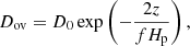 (1)
(1)
where D0 is the diffusion coefficient at the border of the convectively unstable region, z is the distance from the boundary of the convective region, Hp is the pressure scale height, and f is the overshoot parameter set to f = 0.01.
We include turbulent mixing in one of the grids using the prescription of Richer et al. (2000),
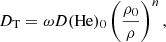 (2)
(2)
where ω and n are constants, ρ and D(He) are the local density and diffusion coefficient of helium, and the index 0 indicates that the value is taken at a reference depth. The D(He) was computed following the analytical expression given by Richer et al. (2000):
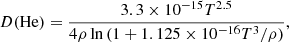 (3)
(3)
where T is the local temperature. In this work, we set ω and n to 104 and 4, respectively (Michaud et al. 2011a,b). We considered the turbulent mixing parameterisation performed by Moedas et al. (2022), where they added the effects of radiative acceleration on iron. These authors used a reference envelope mass (ΔM0, as the reference depth) to indicate the depth that turbulent mixing reaches inside the star. Moedas et al. (2022) suggest that this parameter varies with the mass of the star as
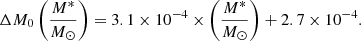 (4)
(4)
Higher values of ΔM0 result in more efficient mixing due to turbulent mixing, which in turn accounts for the radiative acceleration process. For more information, see the work of Moedas et al. (2022; and references therein).
2.2. Parameter space
Both grids cover the same parameter space, with masses ranging between 0.7 and 1.75 M⊙ in steps of 0.05 M⊙, initial metallicities [M/H]i2 from −0.4 to 0.5 dex in steps of 0.05 dex, and an initial helium mass fraction Yi of between 0.24 and 0.34 in steps of 0.01. The two grids differ in terms of the chemical transport mechanisms incorporated. In grid A, turbulent mixing is not included and only atomic diffusion without radiative acceleration is taken into account, and only in models where maximum variation of the iron content at the surface during all the evolution is Δ[Fe/H]3> 0.2 dex. This is to avoid unrealistic, excessive variations caused by atomic diffusion (see Moedas et al. 2022 for more details). Also, by considering Δ[Fe/H], we take into account the effects of changing the initial chemical composition on the efficiency of atomic diffusion (the size of the convective envelope changes with the chemical composition). It is therefore expected that the majority of models of low-mass stars will include atomic diffusion in this grid. All stellar models with mass lower than 1.0 M⊙ are not affected by this criterion and include atomic diffusion. Stars with masses higher than 1.4 M⊙ are all affected and atomic diffusion is not included. For all stellar masses in between, the initial chemical composition is the deciding factor as to whether the model is affected or not, with fewer models including atomic diffusion as stellar mass increases. For example, for models with a mass of 1.3 M⊙, only models with [M/H]i = 0.5 and Yi = 0.24 include atomic diffusion, and for models with a mass of 1.0 M⊙, only models with [M/H]i = −0.4 and Yi = 0.34 do not include atomic diffusion.
In grid B, we include turbulent mixing using the calibration performed in Moedas et al. (2022), where the efficiency of the turbulent mixing increases with stellar mass following Eq. (4). The inclusion of this mechanism allows us to avoid the effects of excessive variation in chemical abundances and to include atomic diffusion in all the stellar models of the grid.
For both grids, we saved the models from the zero-age main sequence (ZAMS) to the bottom of the red-giant branch (RGB) stage. We also computed the individual frequencies for each stellar model using the GYRE oscillation code (Townsend & Teitler 2013). The main properties of the grids are summarised in Table 1.
Parameter space and transport processes of the grids of stellar models.
3. Stellar sample
The sample is selected from two different sources. The first source is the Kepler LEGACY sample from Lund et al. (2017, hereafter L17), which is a sample of 66 stars with the highest signal-to-noise ratio in the seismic frequencies observed by Kepler. The second source is the work of Davies et al. (2016, hereafter D16), a study of 35 stars (32 of them different from L17) that are planet hosts. For both samples, we only selected stars with [Fe/H] > −0.4 to stay within the parameter space of the grids. The smallest value of [Fe/H] is −0.37 dex; we note that the value of [Fe/H] is usually smaller than [M/H] in the stellar models, reaching a difference of up to 0.04 dex, as reported in Moedas et al. (2022), allowing the stars selected to be well within the grid parameter space. We excluded two stars from D16 that present mix-modes in the detection (KIC7199397 and KIC8684730). Finally, we included the degraded Sun as presented in L17 as a control star. Thus, we obtained a sample of 91 stars (62 from L17, 28 from D16, and the Sun). The distribution of the full sample is presented in the asteroseismic diagram of Fig. 1.
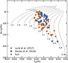 |
Fig. 1. Asteroseismic diagram showing some computed evolutionary tracks with [M/H]i = 0.0 and Yi = 0.26 (that are not the Solar values) in solid black lines. The points show the distribution of the sample considered in this work, where the orange circles are taken from L17, the blue squares are from D16, and the black star is the Sun. |
For all the stars, we use the effective temperature (Teff), iron content ([Fe/H]), frequency of maximum power (νmax), and individual seismic frequencies (νi) as constraints. We use the constraints given in the respective papers, except for 13 stars of L17, for which we use the Teff and [Fe/H] values updated in Morel et al. (2021).
Although the method used to characterise the L17 and D16 samples is the same, the quality of the seismic data for the L17 sample is better because the stars were observed for at least 12 months longer by the Kepler mission. This allows us to see how the data quality will impact the uncertainties in the fundamental stellar property inferences. This aspect is discussed in Sect. 6.2.
4. Optimisation process
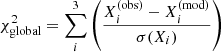
The fundamental properties of the sample defined in the previous section are inferred using both grids in combination with the asteroseismic inference on a massive scale (AIMS, Rendle et al. 2019) code. AIMS is an optimisation tool that uses Bayesian statistics and Markov chain Monte Carlo (MCMC) to explore the grid parameter space and find the model that best fits the observational constraints. In the present work, we use the two-term surface corrections proposed by Ball & Gizon (2014) in order to compensate for the difference between theoretical and observed frequencies, which is due to the incomplete modelling of the surface layers of stars. We also explored the different ways of considering the χ2 in the optimisation. AIMS distinguishes the contribution of the global constraints Xi (in our case Teff, [Fe/H], and νmax),
 (5)
(5)
and the constraints from individual frequencies νi,
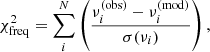 (6)
(6)
where (obs) corresponds to the observed values and (mod) corresponds to the model values. The weight that AIMS gives to the seismic contribution can be absolute (3:N), where each individual frequency has the same weight as each global constraint,
 (7)
(7)
or relative (3:3), where all the frequencies have the same weight as all the global constraints,
 (8)
(8)
where Nglobal and Nfreq are the numbers of global and frequency constraints, respectively.
Cunha et al. (2021) assessed the impact of using these two different ways to consider the weight in the frequencies. The weights 3:3 synthetically inflate the uncertainties of the individual frequencies, which allows the optimisation procedure to explore more of the parameter space. However, this is not statistically correct, as explained in Cunha et al. (2021). If we want the optimisation to be statistically correct, we should instead consider 3:N weights, which use the full potential of the seismic frequencies, leading to results with smaller uncertainties. However, as discussed in Cunha et al. (2021), the use of 3:N weights is more sensitive to an incomplete or incorrect modelling of stars and can lead to results that are incompatible with the global constraints. Given the discussion in the literature around the application of weights, in this work we decided to assess the effect of using both weight options in the results (see Sect. 6.1). The properties of masses, radii, and ages inferred using Grid B are provided in Tables B.1 and C.1 for both (3:N) and (3:3) frequency weights.
5. Results
5.1. The Sun
As a first test, we determined how both grids perform in the inference of the properties of the degraded Sun. This tests the accuracy of the grids in the optimisation process. The results for the Sun are shown in Table 2 and in Fig. 2 for both grids with the consideration of the relative or absolute weights in the frequencies. The results are similar for both grids when we use the same weights in the optimisation. This is expected because the physics is the same for the low-mass models of the grids. In the models of Grid B, the effect of turbulent mixing is negligible, because the convective envelope already fully homogenises the region where it should have an impact. For grid A, most of the models include atomic diffusion. Comparing the same grid but different weights in the frequencies, we see with the 3:3 weights that the true properties of the Sun are within the 1σ uncertainties, except for the radius, which is within 2σ. In contrast, for the 3:N weights, only the radius has the true value within 1σ. For the age it is within 2σ, and for the mass it is within 4σ. From a global perspective, the results are compatible with the current Sun and are in agreement with those obtained by Silva Aguirre et al. (2017).
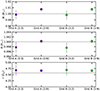 |
Fig. 2. Optimisation results for the Sun: for mass (top panel), radius (middle panel), and age (bottom panel). The dashed line indicates the real value of the Sun. |
Solar properties from the optimisation process.
5.2. Grid comparison
In order to understand how the change of physics (adding turbulent mixing and atomic diffusion for the more massive stars) affects the stellar characterisation, we compare the relative and absolute differences between the fundamental properties inferred with the two grids. In both grids, the inference is made using the 3:N weights of the frequencies in the optimisation because that is the statistically correct option. We estimate the absolute difference with
 (9)
(9)
and the relative difference with
 (10)
(10)
where X is the parameter value that is inferred, XB is the value obtained from grid B, and XA is the reference value obtained from grid A. Figures 3 and 4 show the results for the relative and absolute differences for mass, radius, and age, respectively.
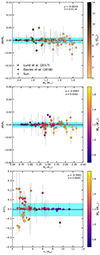 |
Fig. 3. Relative difference for mass (top panel), radius (middle panel), and age (bottom panel) between grids A and B, for 3:N weights. The blue solid line indicates the bias, and the blue region is the 1σ of the standard deviation. Each point is colour coded with the corresponding reference age (top panel) and mass (middle and bottom panels). |
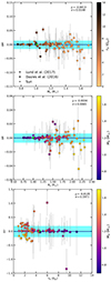 |
Fig. 4. Absolute difference for mass (top panel), radius (middle panel), and age (bottom panel) between grids A and B, for 3:N weights. The blue solid line indicates the bias, and the blue region is the 1σ of the standard deviation. Each point is colour coded with the corresponding reference age (top panel) and mass (middle and bottom panels). |
Globally, we see that the change in physics does not induce a significant bias in the results. Nevertheless, the mean dispersion for age can reach values of about 7%, and the maximum dispersion can reach values of greater than 20%, indicating that the changes in physics have a strong impact on the age determination for individual stars.
We also see that the dispersion in all parameters increases as the stellar mass increases, indicating that the change we made to the grid has indeed impacted the more massive stars. For the lower mass stars, both grids include atomic diffusion and the turbulent mixing prescription has no significant impact (i.e. the turbulent mixing effects are within the convective envelope of these stars).
For the more massive stars, the majority of the models of grid A do not include atomic diffusion. We expect the models with atomic diffusion (grid B) to be affected in two ways. First, the models have a different surface composition at a given age, which has an impact on the inferred stellar properties through the [Fe/H] constraint. Second, atomic diffusion changes the amount of time that the star spends on the main sequence by helping to deplete some of the hydrogen in the core. We see that this can lead to a relative difference for individual stars of greater than 5% in mass, 2% in radius, and 20% in age.
We also look at the absolute differences (Fig. 4) to decipher whether or not the dispersion we see in relative differences at smaller ages is an artefact caused by the computation of a ratio (particularly age; the small reference value in the denominator may mislead the interpretation). We find the same behaviour in the dispersion of the absolute difference, where it increases with stellar mass. The age dispersion can reach differences of more than 0.4 Gyr for the more massive stars, with much larger differences than those found for the lower masses. This leads us to the conclusion that the dispersion in the relative difference is not fully explained by the smaller ages.
In both the relative and absolute cases, we find three outliers for mass and age in low-mass stars. The large difference in these stars is caused by the way Grid A was computed. These stars encounter the border where atomic diffusion is turned off. This creates a discontinuity in the parameter space where models do and do not have atomic diffusion, which leads to greater dispersion in the results for these stars. This reveals that the current way of grid-based modelling – where atomic diffusion is cut at a certain point in the grid in order to avoid excessive variation in chemical surface abundance – will be a source of large uncertainty. The most physically consistent approach is to consider atomic diffusion in all the stellar models whilst considering the other chemical transport mechanisms in competition.
6. Discussion
6.1. Impact of the weight of the frequencies on the inferences
In this section, only grid B is used because both grids give similar results when comparing the inference using 3:N and 3:3 frequency weight. Figure 5 shows the comparison of values inferred using Grid B for the two weight options. The results show that the impact of changing the weights is more significant for the mass and age (top and bottom panels)
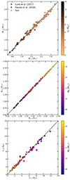 |
Fig. 5. Comparison of the properties inferred when using 3:N or 3:3 weights on the full sample, for mass (top panel), radius (middle panel), and age (bottom panel). Each point is colour coded with the corresponding reference age (top panel) and mass (middle and bottom panels). |
The parameter uncertainties for both cases are presented in the histograms of Fig. 6 for all stars. We find that the two methods give different uncertainty distributions – in accordance with Cunha et al. (2021) – because the use of 3:3 weights is similar to synthetically inflating the uncertainties of the frequencies, as expected. We look at the statistics of the relative differences for the inferred mass, radius, and age between the two cases. The vertical lines in the histograms show the values of the bias (dash-dotted line) and the standard deviation (solid line). There is no significant bias for any of the parameters; all biases are lower than 1%. There is a large scatter in the results of 1.8%, 0.6%, and 6.1% for mass, radius, and age, respectively.
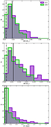 |
Fig. 6. Histogram of uncertainties on the inferred parameters for the full sample and two different weights: mass (top panel), radius (middle panel), and age (bottom panel). The vertical dash-dotted line marks the value of the bias and the vertical solid line marks the value of the standard deviation. |
6.2. Comparison of uncertainties between L17 and D16
In this section, we compare how the quality of the seismic data affects the results, in particular the relationship between the precision of the frequencies and the inferred fundamental properties of the stars. Both L17 and D16 used the same method of seismic identification and quality assurance. The difference is that L17 uses Kepler observations for the stars with the highest signal-to-noise ratios, and therefore the seismic data for this sample are expected to be of better quality.
Figure 7 shows a histogram of the uncertainties for the two sets of stars regarding mass, radius, and age. The D16 sample has a more scattered histogram than the L17 sample and tends to have higher uncertainties, as expected.
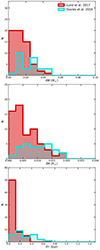 |
Fig. 7. Histogram of uncertainties on the fundamental properties of stars from both samples using the 3:N weights: mass (top panel), radius (middle panel), and age (bottom panel). |
There are three stars in common between the samples (KIC3632418, KIC9414417, and KIC10963065), which can be used to see how the different frequency estimates affect the inference of the results (we used the same Teff and [Fe/H] in the inference, only changing νmax to be consistent with the individual frequency estimate in each work). The results obtained from the seismic data provided by D16 and L17 are presented in Table 3. For the three stars in common, D16 data tend to give smaller values of mass, radius, and age compared to L17 data, and also show a higher uncertainty for these three properties. These differences show that even a small change in the estimated individual frequencies can have a significant impact on the results derived from them. A somewhat surprising finding is that lower masses are linked to lower ages in these three stars from the D16 sample. A possible explanation for this correlation is the difference in the initial chemical compositions ([M/H]i and Yi). For the case of D16, these three stellar models have slightly lower [M/H]i and higher Yi, which may cause the age to be lower for lower estimated masses.
Inferred properties of the stars common to the D16 and L17 samples using the individual frequencies obtained in the respective works.
Uncertainties are expected to decrease with improved quality. This hypothesis was tested on synthetic stars in the work of Cunha et al. (2021), who found that the degraded data gave less accurate results, especially for age determination. This is in agreement with what we find for the Kepler data analysed here.
6.3. Comparison of our results with those of Silva Aguirre et al. (2015, 2017)
In this section, we compare the results obtained using Grid B with those of previous works. We compare our study of the L17 sample with the work of Silva Aguirre et al. (2017) and our study of the D16 sample with the work of Silva Aguirre et al. (2015). In both works, the authors used different pipelines and the grids were built with different codes and input physics. They also use different optimisation codes in each pipeline and use a relative weight for each frequency. Here we compare their results with our results derived using the same relative weight (for consistency).
6.3.1. Comparison with Silva Aguirre et al. (2017)
We compare our results for the L17 sample with the results presented in Silva Aguirre et al. (2017). Here, we show the results for only one of the seven pipelines used in their paper: namely AIMS. Similar conclusions can be drawn for all the others. This pipeline uses the same evolutionary code (MESA) to compute the stellar models as in our work, but with different physical inputs: the stellar models use Grevesse & Noels (1993) solar mixture, an Eddington grey atmosphere, no atomic diffusion, and a fixed helium enrichment ratio ( ).
).
Figure 8 shows the comparison of Grid B results with those from the AIMS pipeline of Silva Aguirre et al. (2017). Our results show a bias towards higher values for mass, radius, and age, with a scatter of 6%, 2%, and 24%, respectively. However, the relative difference for an individual star can be up to 15% for mass, 5% for radius, and 60% for age.
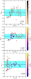 |
Fig. 8. Relative difference for mass (top panel), radius (middle panel), and age (bottom panel) between grid B and the results of Silva Aguirre et al. (2017) for the AIMS pipeline. The blue solid line indicates the bias, and the blue region is the 1σ deviation. Each point is colour coded according to the corresponding reference age (top panel) and mass (middle and bottom panels). |
We also compared the results from Silva Aguirre et al. (2017) with those of grid A in Fig. 9; however, for most cases, we find similar significant bias and scatter as in the comparison with grid B. This suggests that the systematic effects arising from turbulent mixing are overshadowed by the different physics used between our work and Silva Aguirre et al. (2017).
6.3.2. Comparison with Silva Aguirre et al. (2015)
We now compare our results for the stars of D16 with those presented by Silva Aguirre et al. (2015). As in the previous section, the results obtained from all the pipelines in their work were similar and led to the same conclusions. Therefore, we only present a comparison with the BASTA pipeline (Fig. 10) here.
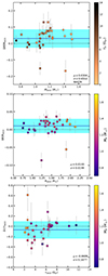 |
Fig. 10. Relative difference for mass (top panel), radius (middle panel), and age (bottom panel) between grid B and Silva Aguirre et al. (2015) results for the BASTA pipeline. The blue solid line indicates the bias, and the blue region is the 1σ deviation. Each point is colour coded according to the corresponding reference age (top panel) and mass (middle and bottom panels). |
We observe a bias towards higher masses and radii, and a bias towards younger ages, with a dispersion of 6%, 2%, and 17% for mass, radius, and age, respectively. For some individual stars, the relative difference can be up to 20% for mass, 10% for radius, and 60% for age.
As before, we also compared the Silva Aguirre et al. (2015) with the results from grid A in Fig. 11. However, we identify a similar bias and scatter as in the comparison with grid B. This again shows that the systematic uncertainties we observe are a consequence of the different physics used between the two works and are not specifically related to the incorporation of turbulent mixing in our grid B.
7. Conclusion
This work is a continuation of the study by Moedas et al. (2022). Our aim is to understand how turbulent mixing and atomic diffusion affects the stellar characterisation of F-type stars. More, precisely, our objective is to study the impact of including calibrated turbulent mixing in stellar models on the derived stellar properties. Including this mechanism allows us to also incorporate atomic diffusion in F-type stars while avoiding excessive variation in surface chemical abundances. To do this, we computed two grids from which we inferred the stellar properties of a sample of FGK-type stars. The first grid (A) neglects atomic diffusion for the F-type stars, while the second grid (B) uses our calibrated turbulent mixing, allowing the use of atomic diffusion in stellar models.
In addition to studying the impact of turbulent mixing, we tested how applying different weights to the seismic data impacts the results. Furthermore, by selecting samples from two different sources, D16 and L17, we investigated how the data quality affects the uncertainties on the properties of observed stars. Finally, we compared our results with those of previous studies that analysed the same samples of stars.
Concerning the combined inclusion of turbulent mixing and atomic diffusion, globally speaking we find no significant impact; that is, a relative bias of less than 1% for masses, radii, and ages. However, we find that there is an increase in the dispersion of the relative differences with mass caused by neglecting atomic diffusion in F-type stars. This can lead to individual relative differences of up to 5% for mass, 2% for radius, and 20% for age. This shows that including atomic diffusion is necessary if we want to avoid this source of uncertainty. We also find three stars that can be considered outliers; their best-fit models are within the limits where atomic diffusion is turned off for grid A for F-type stars. This type of discontinuity in the parameter space introduced in grids by considering models with and without diffusion (such as in our grid A) can therefore introduce significant errors in the inferred stellar properties. Our conclusion is that, in this region of the parameter space, we need the most homogeneous physics across the grid, avoiding discontinuity problems. This result shows that, in order to reduce the uncertainties, we have to consider atomic diffusion in all stellar modes in combination with other chemical-transport mechanisms to avoid unrealistic surface abundance variations. Turbulent mixing is a parameterisation of the different processes and is a step that allows us to improve stellar models and better characterise stars. Although, this improves the prediction of the evolution of iron in stellar models, we still need to take into consideration that it may not be appropriate for other elements (i.e. oxygen and calcium).
The results of other tests we performed on the inference method and data quality are consistent with what was found by Cunha et al. (2021) using synthetic stars. The use of a weight of (3:N) instead of (3:3) for the individual frequency constraints leads to results that are more sensitive to the input physics considered in the stellar models, and to smaller uncertainties, as expected. Our tests show that the better quality of the individual frequencies of L17 provides smaller uncertainties in the inferred properties compared to D16. Our results for the three stars common to both works (KIC3632418, KIC9414417, and KIC10963065) also lead us to a similar conclusion. Nonetheless, the small changes in the determination of the seismic data in these three stars lead to small differences in the inferred values of mass, radius, age, and initial chemical composition.
We compared the results of our sample with previous works. For D16, we compared with the results of Silva Aguirre et al. (2015) and for L17 with Silva Aguirre et al. (2017). We find that there are large differences in both cases, which are due to the different physics adopted in this work compared to in Silva Aguirre et al. (2015, 2017). This reinforces the need for careful consideration of the input physics.
The present work demonstrates that the calibrated turbulent mixing of Moedas et al. (2022) allows a better characterisation of observed F-type stars, even if the proposed scheme is not able to reproduce the chemical evolution of all individual elements. In order to overcome this issue, a further step could be taken, namely the implementation in MESA of the single value parameter (SVP) method (Alecian & LeBlanc 2020), which provides a good balance in efficiency between the calculation of the radiative accelerations and the computation time. Nevertheless, this calibrated turbulent mixing is a step towards a better characterisation of stars with more accurate physics (including atomic diffusion). Finally, with this work, we provide an updated characterisation in terms of the fundamental parameters (mass, radius, and age) for the D16 and L17 stars analysed.
[M/H] = log(Z/X)−log(Z/X)⊙.
[Fe/H] = log(X(Fe)/X)−log(X(Fe)/X)⊙.
Acknowledgments
This work was supported by FCT/MCTES through the research grants UIDB/04434/2020, DOI: 10.54499/UIDB/04434/2020, UIDP/04434/2020, DOI: 10.54499/UIDP/04434/2020, 2022.06962.PTDC., 2022.03993.PTDC, and DOI: 10.54499/2022.03993.PTDC. N.M. acknowledges support from the Fundação para a Ciência e a Tecnologia (FCT) through the Fellowship UI/BD/152075/2021 and POCH/FSE (EC). D.B. acknowledges funding support by the Italian Ministerial Grant PRIN 2022, “Radiative opacities for astrophysical applications”, no. 2022NEXMP8, CUP C53D23001220006. M.C. acknowledges the support by national funds (FCT/MCTES, Portugal), through the contract CEECIND/02619/2017. We also thank Daniel Reese for providing us with the results from AIMS pipeline from Silva Aguirre et al. (2017). We thank the anonymous referee for the valuable comments which helped to improve the paper.
References
- Alecian, G., & LeBlanc, F. 2020, MNRAS, 498, 3420 [NASA ADS] [CrossRef] [Google Scholar]
- Asplund, M., Grevesse, N., Sauval, A. J., & Scott, P. 2009, ARA&A, 47, 481 [NASA ADS] [CrossRef] [Google Scholar]
- Baglin, A., Auvergne, M., Barge, P., et al. 2006, in The CoRoT Mission Pre-Launch Status - Stellar Seismology and Planet Finding, eds. M. Fridlund, A. Baglin, J. Lochard, & L. Conroy, ESA Spec. Publ., 1306, 33 [NASA ADS] [Google Scholar]
- Ball, W. H., & Gizon, L. 2014, A&A, 568, A123 [NASA ADS] [CrossRef] [EDP Sciences] [Google Scholar]
- Borucki, W. J., Koch, D., Basri, G., et al. 2010, Science, 327, 977 [Google Scholar]
- Bressan, A., Marigo, P., Girardi, L., et al. 2012, MNRAS, 427, 127 [NASA ADS] [CrossRef] [Google Scholar]
- Chaboyer, B., Fenton, W. H., Nelan, J. E., Patnaude, D. J., & Simon, F. E. 2001, ApJ, 562, 521 [NASA ADS] [CrossRef] [Google Scholar]
- Cox, J. P., & Giuli, R. T. 1968, Principles of Stellar Structure (Gordon& Breach) [Google Scholar]
- Cunha, M. S., Roxburgh, I. W., Aguirre Børsen-Koch, V., et al. 2021, MNRAS, 508, 5864 [NASA ADS] [CrossRef] [Google Scholar]
- Davies, G. R., Silva Aguirre, V., Bedding, T. R., et al. 2016, MNRAS, 456, 2183 [Google Scholar]
- Deal, M., Alecian, G., Lebreton, Y., et al. 2018, A&A, 618, A10 [NASA ADS] [CrossRef] [EDP Sciences] [Google Scholar]
- Deal, M., Goupil, M. J., Marques, J. P., Reese, D. R., & Lebreton, Y. 2020, A&A, 633, A23 [NASA ADS] [CrossRef] [EDP Sciences] [Google Scholar]
- Dumont, T., Palacios, A., Charbonnel, C., et al. 2021, A&A, 646, A48 [EDP Sciences] [Google Scholar]
- Eggenberger, P., Meynet, G., Maeder, A., et al. 2010, A&A, 519, A116 [CrossRef] [EDP Sciences] [Google Scholar]
- Eggenberger, P., Buldgen, G., Salmon, S. J. A. J., et al. 2022, Nat. Astron., 6, 788 [NASA ADS] [CrossRef] [Google Scholar]
- Ferguson, J. W., Alexander, D. R., Allard, F., et al. 2005, ApJ, 623, 585 [Google Scholar]
- Grevesse, N., & Noels, A. 1993, Phys. Scr. Vol. T, 47, 133 [NASA ADS] [CrossRef] [Google Scholar]
- Gruyters, P., Korn, A. J., Richard, O., et al. 2013, A&A, 555, A31 [NASA ADS] [CrossRef] [EDP Sciences] [Google Scholar]
- Gruyters, P., Nordlander, T., & Korn, A. J. 2014, A&A, 567, A72 [NASA ADS] [CrossRef] [EDP Sciences] [Google Scholar]
- Gruyters, P., Lind, K., Richard, O., et al. 2016, A&A, 589, A61 [NASA ADS] [CrossRef] [EDP Sciences] [Google Scholar]
- Herwig, F. 2000, A&A, 360, 952 [NASA ADS] [Google Scholar]
- Hidalgo, S. L., Pietrinferni, A., Cassisi, S., et al. 2018, ApJ, 856, 125 [Google Scholar]
- Iglesias, C. A., & Rogers, F. J. 1996, ApJ, 464, 943 [NASA ADS] [CrossRef] [Google Scholar]
- Krishna Swamy, K. S. 1966, ApJ, 145, 174 [Google Scholar]
- Lund, M. N., Silva Aguirre, V., Davies, G. R., et al. 2017, ApJ, 835, 172 [Google Scholar]
- Michaud, G., Richer, J., & Richard, O. 2011a, A&A, 529, A60 [NASA ADS] [CrossRef] [EDP Sciences] [Google Scholar]
- Michaud, G., Richer, J., & Vick, M. 2011b, A&A, 534, A18 [NASA ADS] [CrossRef] [EDP Sciences] [Google Scholar]
- Michaud, G., Alecian, G., & Richer, J. 2015, Atomic Diffusion in Stars (Springer) [Google Scholar]
- Moedas, N., Deal, M., Bossini, D., & Campilho, B. 2022, A&A, 666, A43 [NASA ADS] [CrossRef] [EDP Sciences] [Google Scholar]
- Morel, T., Creevey, O. L., Montalbán, J., Miglio, A., & Willett, E. 2021, A&A, 646, A78 [NASA ADS] [CrossRef] [EDP Sciences] [Google Scholar]
- Nsamba, B., Campante, T. L., Monteiro, M. J. P. F. G., et al. 2018, MNRAS, 477, 5052 [NASA ADS] [CrossRef] [Google Scholar]
- Paxton, B., Bildsten, L., Dotter, A., et al. 2011, ApJS, 192, 3 [Google Scholar]
- Paxton, B., Cantiello, M., Arras, P., et al. 2013, ApJS, 208, 4 [Google Scholar]
- Paxton, B., Marchant, P., Schwab, J., et al. 2015, ApJS, 220, 15 [Google Scholar]
- Paxton, B., Schwab, J., Bauer, E. B., et al. 2018, ApJS, 234, 34 [NASA ADS] [CrossRef] [Google Scholar]
- Paxton, B., Smolec, R., Schwab, J., et al. 2019, ApJS, 243, 10 [Google Scholar]
- Pietrinferni, A., Hidalgo, S., Cassisi, S., et al. 2021, ApJ, 908, 102 [NASA ADS] [CrossRef] [Google Scholar]
- Rauer, H., Catala, C., Aerts, C., et al. 2014, Exp. Astron., 38, 249 [Google Scholar]
- Rendle, B. M., Buldgen, G., Miglio, A., et al. 2019, MNRAS, 484, 771 [Google Scholar]
- Richer, J., Michaud, G., & Turcotte, S. 2000, ApJ, 529, 338 [Google Scholar]
- Ricker, G. R. 2016, in AGU Fall Meeting Abstracts, P13C–01 [Google Scholar]
- Rogers, F. J., & Nayfonov, A. 2002, ApJ, 576, 1064 [Google Scholar]
- Salaris, M., & Weiss, A. 2001, A&A, 376, 955 [NASA ADS] [CrossRef] [EDP Sciences] [Google Scholar]
- Semenova, E., Bergemann, M., Deal, M., et al. 2020, A&A, 643, A164 [NASA ADS] [CrossRef] [EDP Sciences] [Google Scholar]
- Silva Aguirre, V., Davies, G. R., Basu, S., et al. 2015, MNRAS, 452, 2127 [Google Scholar]
- Silva Aguirre, V., Lund, M. N., Antia, H. M., et al. 2017, ApJ, 835, 173 [Google Scholar]
- Townsend, R. H. D., & Teitler, S. A. 2013, MNRAS, 435, 3406 [Google Scholar]
- Valle, G., Dell’Omodarme, M., Prada Moroni, P. G., & Degl’Innocenti, S. 2014, A&A, 561, A125 [NASA ADS] [CrossRef] [EDP Sciences] [Google Scholar]
- Valle, G., Dell’Omodarme, M., Prada Moroni, P. G., & Degl’Innocenti, S. 2015, A&A, 575, A12 [NASA ADS] [CrossRef] [EDP Sciences] [Google Scholar]
- Verma, K., & Silva Aguirre, V. 2019, MNRAS, 489, 1850 [NASA ADS] [CrossRef] [Google Scholar]
- Vick, M., Michaud, G., Richer, J., & Richard, O. 2010, A&A, 521, A62 [EDP Sciences] [Google Scholar]
- Weiss, A., & Schlattl, H. 2008, Ap&SS, 316, 99 [CrossRef] [Google Scholar]
Appendix A: Grid comparison 3:3 frequency weight
Figures A.1 and A.2 are the same as Figs. 3 and 4 but for the 3:3 weights. In this case, we can see the same behaviour as in the case of the 3:N weights. However, we can see that for the case of relative weights, there is a smaller dispersion (which we can see in the standard deviation). This is due to the fact that the use of absolute weights leads to greater sensitivity to the input physics. Nevertheless, the conclusion we obtain using the 3:N or 3:3 weights in frequencies is the same, and is simply more pronounced for the 3:N weights.
Appendix B: Fundamental properties using 3:N frequency weighting
Inferred fundamental properties of the stars using 3:N frequency weighting.4
Appendix C: Fundamental properties using 3:3 frequency weighting
Inferred fundamental properties of the stars using 3:3 frequencies weight.5
All Tables
Inferred properties of the stars common to the D16 and L17 samples using the individual frequencies obtained in the respective works.
All Figures
|
Fig. 1. Asteroseismic diagram showing some computed evolutionary tracks with [M/H]i = 0.0 and Yi = 0.26 (that are not the Solar values) in solid black lines. The points show the distribution of the sample considered in this work, where the orange circles are taken from L17, the blue squares are from D16, and the black star is the Sun. |
| In the text | |
|
Fig. 2. Optimisation results for the Sun: for mass (top panel), radius (middle panel), and age (bottom panel). The dashed line indicates the real value of the Sun. |
| In the text | |
|
Fig. 3. Relative difference for mass (top panel), radius (middle panel), and age (bottom panel) between grids A and B, for 3:N weights. The blue solid line indicates the bias, and the blue region is the 1σ of the standard deviation. Each point is colour coded with the corresponding reference age (top panel) and mass (middle and bottom panels). |
| In the text | |
|
Fig. 4. Absolute difference for mass (top panel), radius (middle panel), and age (bottom panel) between grids A and B, for 3:N weights. The blue solid line indicates the bias, and the blue region is the 1σ of the standard deviation. Each point is colour coded with the corresponding reference age (top panel) and mass (middle and bottom panels). |
| In the text | |
|
Fig. 5. Comparison of the properties inferred when using 3:N or 3:3 weights on the full sample, for mass (top panel), radius (middle panel), and age (bottom panel). Each point is colour coded with the corresponding reference age (top panel) and mass (middle and bottom panels). |
| In the text | |
|
Fig. 6. Histogram of uncertainties on the inferred parameters for the full sample and two different weights: mass (top panel), radius (middle panel), and age (bottom panel). The vertical dash-dotted line marks the value of the bias and the vertical solid line marks the value of the standard deviation. |
| In the text | |
|
Fig. 7. Histogram of uncertainties on the fundamental properties of stars from both samples using the 3:N weights: mass (top panel), radius (middle panel), and age (bottom panel). |
| In the text | |
|
Fig. 8. Relative difference for mass (top panel), radius (middle panel), and age (bottom panel) between grid B and the results of Silva Aguirre et al. (2017) for the AIMS pipeline. The blue solid line indicates the bias, and the blue region is the 1σ deviation. Each point is colour coded according to the corresponding reference age (top panel) and mass (middle and bottom panels). |
| In the text | |
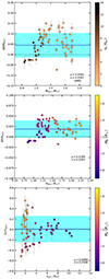 |
Fig. 9. Same as Fig. 8 but using our results from Grid A. |
| In the text | |
|
Fig. 10. Relative difference for mass (top panel), radius (middle panel), and age (bottom panel) between grid B and Silva Aguirre et al. (2015) results for the BASTA pipeline. The blue solid line indicates the bias, and the blue region is the 1σ deviation. Each point is colour coded according to the corresponding reference age (top panel) and mass (middle and bottom panels). |
| In the text | |
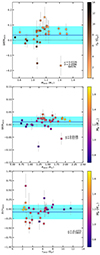 |
Fig. 11. Same as Fig. 10 but using our results from Grid A. |
| In the text | |
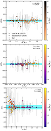 |
Fig. A.1. Same as Fig. 3 but using 3:3 weights for frequencies. |
| In the text | |
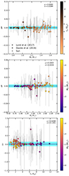 |
Fig. A.2. Same as Fig. 4 but using 3:3 weights for frequencies |
| In the text | |
Current usage metrics show cumulative count of Article Views (full-text article views including HTML views, PDF and ePub downloads, according to the available data) and Abstracts Views on Vision4Press platform.
Data correspond to usage on the plateform after 2015. The current usage metrics is available 48-96 hours after online publication and is updated daily on week days.
Initial download of the metrics may take a while.