| Issue |
A&A
Volume 684, April 2024
|
|
|---|---|---|
| Article Number | A67 | |
| Number of page(s) | 7 | |
| Section | Astrophysical processes | |
| DOI | https://doi.org/10.1051/0004-6361/202348482 | |
| Published online | 03 April 2024 | |
Soft-state optical spectroscopy of the black hole MAXI J1305-704
1
Dipartimento di Scienze Fisiche ed Astronomiche, Università di Palermo, Via Archirafi 36, 90123 Palermo, Italy
2
INAF/IASF Palermo, Via Ugo La Malfa 153, 90146 Palermo, Italy
e-mail: This email address is being protected from spambots. You need JavaScript enabled to view it.
3
IRAP, Université de Toulouse, CNRS, UPS, CNES, 9, Avenue du Colonel Roche BP 44346, 31028 Toulouse, Cedex 4, France
4
Instituto de Astrofísica de Canarias, 38205 La Laguna, Tenerife, Spain
5
Departamento de Astrofísica, Univ. de La Laguna, 38206 La Laguna, Tenerife, Spain
6
Institut d’Estudis Espacials de Catalunya (IEEC), Carrer Gran Capità 2-4, 08034 Barcelona, Spain
7
Institute of Space Sciences (ICE, CSIC), Campus UAB, Carrer de Can Magrans s/n, 08193 Barcelona, Spain
8
Anton Pannekoek Institute for Astronomy, University of Amsterdam, Postbus 94249, 1090 GE Amsterdam, The Netherlands
9
Department of Astronomy, University of Michigan, 1085 South University Avenue, Ann Arbor, MI 48109, USA
10
Department of Astronomy, Ohio State University, 140 W 18th Avenue, Columbus, OH 43210, USA
11
Department of Physics, University of Trento, Via Sommarive 14, 38122 Povo (TN), Italy
Received:
3
November 2023
Accepted:
25
January 2024
Abstract
The X-ray dipper MAXI J1305-704 is a dynamically confirmed black hole (BH) X-ray binary discovered a decade ago. While its only outburst has been studied in detail in X-rays, follow-up at other wavelengths has been scarce. We report here the results from an optical spectroscopy campaign across the outburst of MAXI J1305-704. We analysed two epochs of data obtained by the Magellan Clay Telescope during two consecutive nights, when the source was in a soft X-ray spectral state. We identified typical emission lines from outbursting low-mass X-ray binaries, such as the hydrogen Balmer series, He II 4686 Å and the Bowen blend. We focused our analysis on the prominent Hα line, which exhibits asymmetric emission and variable absorption components. We applied both traditional analytical methods and machine-learning techniques in order to explore the association of the absorption features with outflowing phenomena, and we conclude that they are best explained by broad absorption. This result is consistent with reports from other outbursting BHs, where optical outflows have predominantly been observed in the hard state. Further observations at different X-ray states are key to properly test whether this behaviour is universal and to determine the implications for the disc wind physics.
Key words: accretion, accretion disks / stars: black holes / X-rays: binaries
© The Authors 2024
 Open Access article, published by EDP Sciences, under the terms of the Creative Commons Attribution License (https://creativecommons.org/licenses/by/4.0), which permits unrestricted use, distribution, and reproduction in any medium, provided the original work is properly cited.
This article is published in open access under the Subscribe to Open model. This email address is being protected from spambots. You need JavaScript enabled to view it. to support open access publication.
1. Introduction
Low-mass X-ray binaries (LMXBs) are binary systems composed of a compact object [either a black hole, BH, or a neutron star] and a donor star (M ≲ 1 M⊙) that transfers mass onto the compact object via an accretion disc. Hundreds of LMXBs (Avakyan et al. 2023) have been found since the onset of X-ray astronomy (Giacconi et al. 1962), but barely 70 of them have been flagged as candidates for harbouring BHs. Of these 70 LMXBs, 19 are dynamically confirmed (see Corral-Santana et al. 2016; Torres et al. 2019; Mata Sánchez et al. 2021). They are typically found to be transient systems and spend most of their lives in a faint quiescent state, but they show occasional outbursts. These are short-lived periods during which their brightness increases by orders of magnitude across all wavelengths. Observations in quiescence enable dynamical studies (Casares 2001), while research dedicated to their outbursts has revealed extreme accretion and ejection phenomena (see e.g. Fender & Muñoz-Darias 2016 for a review).
During the past decade, the study of outflows during outburst has taken a pivotal position in the field, as it sparked the debate about their role in regulating this active period. They have further been proposed to impact the overall LMXB evolutionary history through removal of angular momentum and through their contribution to the mass accretion budget (see e.g. Gallegos-Garcia et al. 2023). Multi-wavelength features associated with outflows were discovered across the energy spectrum. They were associated with radio jets dominating the hard state and/or with X-ray winds appearing during the soft state (e.g. Fender 2006; Parra et al. 2024). The latter are characterised by blueshifted absorption features of highly ionised species, and their predominant detection in the soft states of high-inclination systems led to the hypothesis of an equatorial outflow geometry (e.g. Miller et al. 2006; Neilsen & Lee 2009; Ponti et al. 2012). However, some simulations are able to explain the observables with spherically symmetric winds (e.g. Higginbottom et al. 2018).
A few years ago, cold accretion disc winds were found in the optical spectra of high-inclination LMXBs obtained during the hard state (Muñoz-Darias et al. 2016; see also Muñoz-Darias & Ponti 2022 for the connection with X-ray winds). Since then, similar features have been observed in a variety of systems, mainly detected as P-Cygni profiles, but also as broad wings and flat-top profiles, all of them signatures of outflowing material (see Panizo-Espinar et al. 2022 for a compilation). The increasing interest of the community in these features has ultimately enabled a rising number of detections at other wavelengths, including in the near-IR (NIR; e.g. Sánchez-Sierras & Muñoz-Darias 2020; Mata Sánchez et al. 2022) and the UV (Castro Segura et al. 2022). This has led to the hypothesis that accretion disc winds in LMXBs are multi-phase in nature (see Muñoz-Darias & Ponti 2022). The prolific detection of unambiguous wind features in the optical spectra, especially for high-inclination systems, led to the hypothesis that their detection is associated with the hard state. However, several of these systems displayed a hard-state outburst alone (V404 Cyg, Muñoz-Darias et al. 2016; V4641 Sgr, Muñoz-Darias et al. 2018; GRS 1716-249, Cúneo et al. 2020; Swift J1357.2-0933, Jiménez-Ibarra et al. 2019a). The number of optical spectra obtained during the soft state of the remaining sources is quite limited, which has prevented us from properly testing whether winds during this state can be observed in the optical range. NIR observations during the soft state suggest that low-ionisation (cold) winds are active all the time (Sánchez-Sierras & Muñoz-Darias 2020).
MAXI J1305-704 (hereafter J1305) was proposed to be a high-inclination BH X-ray binary in view of its X-ray properties (e.g. dipping behaviour) during outburst (Suwa et al. 2012; Kennea et al. 2012; Shidatsu et al. 2013; Morihana et al. 2013). The source was first detected by the Monitor of All-sky X-ray Image instrument (MAXI; Matsuoka et al. 2009), which is equipped with the Gas Slit Camera (GSC; Mihara et al. 2011) as part of its transient-alert system, on April 9, 2012 (Suwa et al. 2012). Subsequent follow-up observations performed with the Neil Gehrels Swift Observatory (Gehrels 2004) confirmed an uncatalogued bright X-ray source by both its onboard X-Ray Telescope (XRT; Burrows et al. 2005) and the UltraViolet and Optical telescope (UVOT; Roming et al. 2005). Miller et al. (2014) reported a potential failed wind in the X-rays during the hard state of this system, making it a promising candidate for the search of multi-wavelength outflow signatures. An optical study during quiescence provided dynamical confirmation of a BH accretor, determined the orbital period (Porb = 0.394 ± 0.004 d), and further supported the high-inclination scenario (Mata Sánchez et al. 2021).
The outburst of J1305 has been studied in detail in X-rays, but follow-up in other wavelengths has been scarce. Shaw et al. (2017) presented the only published optical spectrum during outburst, with limited spectral coverage during the hard-to-soft transition. In this work, we report our analysis of two optical spectroscopic epochs. They allow us to study the possible presence of outflow features in this high-inclination system during the soft state for the first time, which is a key task to continue to build a complete picture of the physics of the outflows.
2. Observations and data reduction
We observed J1305 during its discovery outburst in 2012 with the 6.5 m Magellan Clay telescope (PI: Degenaar) at the Las Campanas Observatory (Chile). We employed the Low Dispersion Survey Spectrograph (LDSS-3) and the VPH-ALL Grism setup. All observations used a 0.75″ slit, which resulted in a resolving power of R = 826, measured as the full width at half maximum (FWHM) of the skylines from the background spectra. We observed the system during two consecutive nights, May 2 (02:18:34 UTC to 02:56:41 UTC) and May 3 (00:29:36 UTC to 01:09:03 UTC). The exposure time of each individual spectrum was fixed to 300 s, amounting to six spectra per epoch. This setup allowed us to cover a broad wavelength range (4300–11 000 Å). We reduced the data using standard procedures based on the IRAF 1 software, MOLLY tasks, and PYTHON packages from ASTROPY and PYASTRONOMY (Astropy Collaboration 2022). They allowed us to correct the observed spectra for bias and flats, as well as to calibrate them in wavelength using Ne, He, and Ar lamps.
To place our observations in context, we analysed publicly available Swift data. We analysed the Swift/XRT observation on May 3, 2012, coincident with the second day of our optical data set, using standard recipes from the Swift XRTPIPELINE v6.32.12. The processed event files were generated, and a circular region of 47″ was selected for both the source and background, positioned around and away from the source, respectively. We used the tool XRTPRODUCTS to extract the spectrum, which was binned with the tool GRPPHA to have a sufficient number of counts in each bin. We employed a proper ancillary response file (ARF) and redistribution matrix files (RMF) to model the spectrum with the X-ray spectrum-fitting program XSPEC (Arnaud 1996).
We also analysed publicly available UVOT data spanning from April 11 to July 14, 2012. UVOT has the following filters: U, B, and V in the optical, and UVW1, UVM2, and UVW2 (W2) in the ultraviolet band. We selected a region of 5″ around the source and a combination of small regions away from the source to define the background. Then, we used the task UVOTSOURCE, which provides the coincidence-corrected count rate, magnitude, and flux density.
3. Analysis and results
3.1. X-ray spectral state
We employed publicly available MAXI3 data collected from April 5 to July 17, 2012, corresponding to the initial and decay phases of the outburst, respectively (Morihana et al. 2013). The X-ray light curve and hardness ratio are shown in Fig. 1. We selected 2 − 4 keV and 4 − 10 keV energy bands to define the soft and hard colours in the hardness ratio, while the 2 − 10 keV energy band traces the system brightness. We binned the data into one-day intervals during the MJD 56022–56034 period, while we use five-day intervals for the remaining (and fainter) epochs to increase the signal-to-noise ratio (S/N). A complete hardness-intensity diagram using these same energy bands is available in (Morihana et al. 2013; see Fig. 3). The hard-to-soft transition occurred around 20 days prior to our optical observations (Suwa et al. 2012), which lies within interval D defined in Morihana et al. (2013). The X-ray spectra obtained two weeks prior to our observations already reveal properties consistent with a high-soft state (Shidatsu et al. 2013). This is further supported by the standard analysis of a Swift/XRT observation on May 3, which is simultaneous with our optical data set. We fit the 0.5–10.0 keV spectrum with a disc black-body model plus a power law absorbed at low energies, both corrected from the interstellar absorption using the TBABS model provided by XSPEC. We also included a Gaussian in the model to reproduce a broad absorption at ∼1 keV. While this is reminiscent of the features found by Miller et al. (2014) based on Chandra/HETG data, the association with a failed X-ray wind is uncertain due to the limited spectral resolution of our data set, and so we decided to focus on the continuum alone. The resulting model TBABS*(DISKBB+EXPABS*POWERLAW+GAUSSIAN) provides spectral parameters typical of soft states in BH binaries, that is, a disc temperature of kTin = 0.91 ± 0.03 keV plus a steep power law (Γ above 3). Assuming a BH mass of 10 M⊙ and a distance of 7.5 kpc (Mata Sánchez et al. 2021), we derive a bolometric luminosity of 8 × 1038 erg s−1, which results in ∼0.4 LEdd.
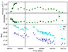 |
Fig. 1. X-ray and UV/optical light curves of the source. Top panel: Light curve of MAXI J1305-704 from the 2 − 10 keV band count rate provided by MAXI. Middle panel: Hardness-ratio data constructed from the 2 − 4 keV and 4 − 10 keV energy band count rate provided by MAXI. Bottom panel: UVOT light curve in the W2 ultraviolet and B optical band. The dotted black and red lines represent our optical observations of epochs A and B, respectively. |
3.2. Optical spectra
We used tailored PYTHON routines to normalise the observed spectra. The selected LDSS-3 setup produced spectra covering a wide wavelength range. It also introduced an instrumental offset in the continuum between the regions covered by its two CCDs, however: 4300–6600 Å (CCD2) and 6600–11.000 Å (CCD1). To account for this misalignment on the continuum level, we normalised the spectra using a function compounded of a fifth-grade polynomial and a step function at the point of the misalignment. The resulting averaged normalised spectra for the two consecutive nights of observations (hereafter, epochs A and B, respectively) are shown in Fig. 2. While the full optical spectra cover a range from 4300 to 11 000 Å, the lack of relevant features, the presence of telluric absorption, and the S/N limitations caused us to focus on the region from 4500 to 6950 Å.
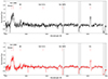 |
Fig. 2. Average spectra of epoch A (black) and epoch B (red) of the optical observations. The light grey band on the left corresponds to the edge of the 5890 sodium D line, while the other two bands correspond to the strongest telluric absorption. |
We identify hydrogen emission lines from the Balmer series Hα (see Fig. 3) and a weaker Hβ. High-excitation lines are also present, such as He II 4686 Å (Fig. 2) and the Bowen blend (a mixture of the N III and C III emission lines resulting from fluorescence cascades; see e.g. Steeghs & Casares 2002). These are consistent with the soft-state classification derived from Morihana et al. (2013).
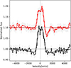 |
Fig. 3. Average Hα emission line of epochs A (black, bottom) and B (red, top). The solid lines are the best fit to the nightly average (see Table 1 for the precise parameters). The normalised profiles have been separated vertically by a constant offset for visual purposes. |
We focused our analysis on the Hα line, which is the strongest isolated feature in all our spectra. The line profile exhibits a clear evolution, both within each observed spectrum (Fig. 4) and between epochs (Fig. 3). It can be described as a double-peaked emission line, as expected from a Keplerian accretion disc (Smak 1981), superimposed on an underlying and variable absorption component. Both Figs. 3 and 4 show that the first epoch shows a blueshifted absorption in at least two spectra (1A and 2A, and potentially 4A), while in the second epoch, the absorption appears to be redshifted. To better understand the evolution of the line profile, we performed a multi-Gaussian fit to the Hα line using the PYTHON curve-fit routine from the SCIPY package (Virtanen et al. 2020). To reproduce the emission component, we fit each spectrum with two Gaussians with the following parameters: the peak height of the Gaussians, the FWHM (linked between Gaussians), the centroid of the combined profile (offset), and the double-peak separation (DP). In order to reproduce the absorption component present in a significant part of our sample, we included in the model a third Gaussian in absorption, with independent and free parameters; for the absorption Gaussian, we set the parameters depth, FWHM, and offset. The results of the fit are collected in Table 1 (see also Fig. 3 for an example of the fitted model). We do not report the fit parameters for absorption components whose depth was shallower than 0.02 because this corresponds to less than twice the S/N measured on the nearby continuum (S/N = 80 for our individual spectra), and we therefore deemed them unreliable. Examining these values, we find that spec 1A is the only clear example with a significant narrow blueshifted absorption. During epoch B, almost all spectra display redshifted absorption with depths exceeding 3σ. The terminal velocity of the absorption components, defined as one FWHM away from the centroid of the absorption feature, is comparable between the two epochs (∼1300 − 1600 km s−1), but with the opposite sign.
 |
Fig. 4. Individual Hα emission lines from the spectra obtained during epoch A (black) and epoch B (red) of the optical observations. The dotted black lines mark the maximum terminal velocity observed in the blueshifted and redshifted absorption features (±1500 km s−1). The solid red line marks the intersection between CCDs, proving that the redshifted features, when present, are not due to a normalisation issue. The normalised profiles have been separated vertically by a constant offset for visual purposes. |
Best-fit parameters of the multi-Gaussian model described in the text, applied to our two observation epochs.
We also analysed the nightly average spectra of the Hβ line, which reveals an FWHM and DP consistent with those of Hα. Because the S/N of the former is lower, we limit our discussion to the Hα line.
3.3. Swift/UVOT: Search for orbital UV modulation
The Hα line profile undergoes rapid changes within a few minutes and between epochs (see Fig. 4). Although the double-peaked emission component is not highly asymmetric, the varying intensity from peak to peak suggests a potential hot spot on the disc. To explore this possibility, we analysed publicly available UVOT data from April 11 to July 14, 2012, and extracted the corresponding light curve with the data binned in one-day intervals in all available bands. The photometric light curves in the B and W2 filters are shown in Fig. 1 (bottom panel) as a proxy for the simultaneous system brightness in the optical and UV wavelengths during the outburst event. We searched for superhumps near the orbital period (Porb = 0.394 ± 0.004 d; Mata Sánchez et al. 2021) in the light curve because these features are commonly associated with the aforementioned hot-spot structures. An inspection of the light curve with dedicated tools (e.g., EFSEARCH and EFOLD from HEASARC) did not reveal any significant modulation.
The temporal gap between the quiescence observations establishing the J1305 ephemeris (Mata Sánchez et al. 2021) and our earlier outburst data set, combined with the uncertainty in Porb, prevented us from maintaining coherence and calculating absolute orbital phases. Instead, we defined the relative orbital phases with respect to the first epoch of observations. Following this convention, we observed the spectra covering orbital phases between 0.0–0.06 in epoch A and between 2.35–2.41 during epoch B. Unfortunately, our coverage of the orbit is not extensive enough to thoroughly assess the association of the profile variability with the orbital period. Nevertheless, the relatively rapid variability of the profile peaks, which change within the span of a single epoch, suggests that a single hot spot might not be sufficient to explain the observed behaviour.
4. Discussion
We present two epochs of optical spectroscopy obtained during the soft state of J1305 for the first time. These observations reveal a prominent Hα line profile, accompanied by an absorption component of varying intensity in each exposure. For this reason, we now explore the association of these features with outflow phenomena.
4.1. Search for optical wind features
The most outstanding feature associated with cold winds in LMXBs are P-Cygni profiles, although other signatures (e.g., flat-top profiles or broad wings) have traditionally been considered as markers for the presence of outflows (see Panizo-Espinar et al. 2022 for a compilation). The spectra of epochs A and B exhibit significant differences, and the Hα line profile shows variability within a timescale of a few minutes. Individual inspection reveals a clear blueshifted absorption in at least one spectrum (1A; see Fig. 4), down to 5% below the continuum level. While it is tempting to associate this with a P-Cygni profile, there are a few indicators that prevent us from doing so.
Only a single spectrum of our spectroscopic data set shows a clear detection of this feature, while deep redshifted absorption is consistently present during epoch B. The outflow interpretation for the former would also suggest that most of the epoch B spectra possess inverted P-Cygni profiles, which are elusive features associated with inflows that were only reported in one LMXB so far (Cúneo et al. 2020). This is of particular interest due to the potential presence of failed X-ray winds proposed for this very system when it was in a hard state (Miller et al. 2014). Nevertheless, the terminal velocities associated with the X-ray features are higher by an order of magnitude than those found in the optical. This suggests that they do not trace the same phenomena, given that systems in which X-ray and optical winds coexist seem to show similar terminal velocities (e.g. Muñoz-Darias & Ponti 2022).
The comparison of the blue- and redshifted absorption features in the optical spectra instead shows a perfect agreement in depth and terminal velocity (∼1300 − 1600 km s−1). The multi-Gaussian fit performed on our sample and compiled in Table 1 reveals absorption components with large FWHMs in a significant number of our exposures (e.g. 2B). Their terminal velocities are also consistent with the remaining examples of narrow redshifted absorption (e.g. 3B), and together, they support a common origin for all absorption features.
Following the above reasons, and given the lack of other wind-sensitive lines in the spectra with good enough S/N (e.g., He I 5876 Å), we disfavour an outflow interpretation. Instead, we propose that an underlying broad and fast-changing absorption component might be the main driver of the profile variability in the whole data set. A feature like this is able to produce both the apparent narrow redshifted absorption observed in epoch B and the blueshifted absorption observed in epoch A spectra as a result of different offset parameters for the emission and absorption components. The lack of ouflows is consistent with the current paradigm, where they have not been detected at optical wavelengths during the soft state of any LMXB, possibly due to the outflow ionisation conditions (Muñoz-Darias & Ponti 2022). Nevertheless, outflow-related signatures have previously been reported in the NIR, indicating that the wind is still present during this state, although it reveals itself in different energy ranges (Sánchez-Sierras & Muñoz-Darias 2020).
We note that our results do not allow us to definitively rule out the presence of winds during the outburst of J1305 because our temporal coverage is quite restricted and does not even cover a complete orbital phase. Some flat-top profiles (e.g. spectra 2A and 3A) might tentatively be associated with winds. However, our limitation to studying a single emission line prevents us from providing a definitive confirmation.
4.2. Machine-learning test
The analytical fits to the spectra are not fully conclusive and prevent us from efficiently distinguishing between the outflow and broad absorption scenarios. In an attempt to minimise biases depending on the observer interpretation, we employed the deep neural network classifier ATM (Mata Sánchez et al. 2023). This independent method is trained to classify any given spectrum as one of the following five types: disc (without outflows); blue-absorption, broad, and P-Cygni (three classes containing different examples of outflow features); and absorbed (a dedicated class for the broad absorption case). It is important to note that ATM is trained to detect features with a relative strength of at least 3σ above the noise level (σ = 0.01). For this reason, we decided to follow a Monte Carlo approach to better assess the impact on the classification of the S/N (see Sect. 4.3 in Mata Sánchez et al. 2023). The application to the J1305 data revealed two potential blue absorption profiles during epoch A (1A and 4A), although it reports a similar probability to belong to the absorbed class. The remaining spectra are all classified as absorbed, which suggests that broad absorption is ubiquitous within our data set. Because the absolute terminal velocities of all features, whether blue- or redshifted, are consistent in epochs A and B, we again favour the broad absorption interpretation for the current sample. This result is further supported through the application of the ATM classifier to the daily averaged spectra, which reveals that the two epochs are of the absorbed type.
4.3. Origin of the broad absorption features
The origin of this broad absorption is not well understood to date, but it has been observed in several LMXBs (e.g. GRS 1009-45; della Valle et al. 1997; GRO J1655-40; Soria et al. 2000; and MAXI J1807+132; Jiménez-Ibarra et al. 2019b). The most widely accepted explanation for the origin of these features was introduced in Dubus et al. (2001). This scenario requires a region in the system that behaves like a stellar atmosphere to produce the absorption component while simultaneously retaining the hotter irradiated disc atmosphere that causes the canonical double-peaked emission lines. The conditions for both components to coexist pose a challenge when trying to develop an analytical model to explain them. Another issue is the broad width of the observed absorption component, which could arise from either a Doppler shift or electronic pressure. In the first case, the absorbing structure has to be located at a radius closer to the BH than that of the emission region to produce a broader absorption than the emission component. Moreover, it should be extended and non-homogeneous to reproduce the observed variability in the spectra. A possibility of reconciling the two might be a structure shielding some regions of the outer accretion disc, but no detailed modelling has been done to date.
The Dubus et al. (2001) scenario proposed an origin in electronic pressure, but their model is still not sufficient to fully explain the observations. In particular, it predicts that the observation of these features should be favoured in low-inclination systems. Nevertheless, all the dynamically confirmed BHs with a high orbital inclination (i ≳ 65 deg) have shown broad absorption features at some epoch during their outburst: XTE J1118+480 (i = 68 − 79 deg, Dubus et al. 2001; Khargharia et al. 2013), MAXI J1659-152 (i = 70 − 80 deg, Torres et al. 2021; Kaur et al. 2012), and now J1305 ( ; Mata Sánchez et al. 2021). When we extend our analysis to BH candidates with an X-ray dipping nature (considered strong proof of a high orbital inclination), the list is further augmented with MAXI J1803-298 (Mata Sánchez et al. 2022).
To further progress in our understanding of these features and to reconcile predictions and observations, two avenues should be explored. On one hand, new models providing testable predictions are required. On the other hand, follow-up of new outburst events is key to exploring the orbital dependence (if any) on the broad absorption evolution, as well as to inspect outflows by comparing different line profiles. In the J1305 optical spectra, we also identify the He II 4686 Å and a weaker Hβ emission line (see Fig. 2). However, the nearby Bowen blend for the former and the much lower S/N for the latter prevent us from drawing relevant conclusions on the presence of outflows, showing that at least 8 m class telescopes are required for more detailed studies.
5. Conclusions
We presented the analysis of the optical spectroscopy obtained during the outburst of J1305. We reduced the data collected during two consecutive nights of observations when the source was in the soft state (Morihana et al. 2013). This aligns with the overall characteristics of the optical spectra, featuring high-excitation emission lines such as the He II 4686 line and the Bowen blend.
We focused our analysis on the Hα line as the strongest isolated feature in the spectra. We modelled it with a multi-Gaussian fit to better understand its evolution, and we concluded that it can be described as a double-peaked emission and a broad absorption component. This interpretation is favoured over a P-Cygni detection during the epochs exhibiting blueshifted absorption components. An independent classification using the ATM machine-learning algorithm further supported this conclusion. While broad absorption has been observed in various LMXBs, the traditional theoretical explanation contradicts their observation in a growing sample of high-inclination systems, to which J1305 is now added.
The non-detection of conclusive outflow features in J1305 in the soft state remains consistent with the picture built over the past few years. However, it is still a matter of debate that requires further observations of outbursting systems to be settled. In this regard, this paper serves as a cautionary tale and highlights the key role of multi-epoch observations to confidently identify outflow signatures. Detailed observations with improved temporal cadence during future outbursts of the source are encouraged to better understand the complex evolution of the Hα line.
IRAF is distributed by the National Optical Astronomy Observatories, operated by the Association of Universities for Research in Astronomy, Inc., under contract with the National Science Foundation.
Acknowledgments
D.M.S., T.M.D. and M.A.P. acknowledge support by the Spanish Ministry of Science via the Plan de Generacion de conocimiento PID2020-120323GB-I00 and PID2021-124879NB-I00, as well as a Europa Excelencia grant (EUR2021-122010). A.M. is supported by the H2020 ERC Consolidator Grant “MAGNESIA” under grant agreement No. 817661 (PI: Rea) and National Spanish grant PGC2018-095512-BI00. A.M. acknowledges also partial support from grant SGR2021-01269 (PI: Graber). This work was also partially supported by the program Unidad de Excelencia Maria de Maeztu CEX2020-001058-M, and by the PHAROS COST Action (No. CA16214). This research has made use of MAXI data provided by RIKEN, JAXA and the MAXI team. We thank Tom Marsh for the use of MOLLY software.
References
- Arnaud, K. A. 1996, in Astronomical Data Analysis Software and Systems V, eds. G. H. Jacoby, & J. Barnes, ASP Conf. Ser., 101, 17 [NASA ADS] [Google Scholar]
- Astropy Collaboration (Price-Whelan, A. M., et al.) 2022, ApJ, 935, 167 [NASA ADS] [CrossRef] [Google Scholar]
- Avakyan, A., Neumann, M., Zainab, A., et al. 2023, A&A, 675, A199 [NASA ADS] [CrossRef] [EDP Sciences] [Google Scholar]
- Burrows, D. N., Hill, J. E., Nousek, J. A., et al. 2005, Space Sci. Rev., 120, 165 [Google Scholar]
- Casares, J. 2001, in Binary Stars: Selected Topics on Observations and Physical Processes, eds. F. C. Lázaro, & M. J. Arévalo, Lect. Notes Phys., 563, 277 [NASA ADS] [CrossRef] [Google Scholar]
- Castro Segura, N., Knigge, C., Long, K. S., et al. 2022, Nature, 603, 52 [NASA ADS] [CrossRef] [Google Scholar]
- Corral-Santana, J. M., Casares, J., Muñoz-Darias, T., et al. 2016, A&A, 587, A61 [NASA ADS] [CrossRef] [EDP Sciences] [Google Scholar]
- Cúneo, V. A., Muñoz-Darias, T., Sánchez-Sierras, J., et al. 2020, MNRAS, 498, 25 [CrossRef] [Google Scholar]
- della Valle, M., Benetti, S., Cappellaro, E., & Wheeler, C. 1997, A&A, 318, 179 [NASA ADS] [Google Scholar]
- Dubus, G., Kim, R. S. J., Menou, K., Szkody, P., & Bowen, D. V. 2001, ApJ, 553, 307 [NASA ADS] [CrossRef] [Google Scholar]
- Fender, R. 2006, in Relativistic Jets: The Common Physics of AGN, Microquasars, and Gamma-Ray Bursts, eds. P. A. Hughes, & J. N. Bregman, AIP Conf. Ser., 856, 23 [NASA ADS] [CrossRef] [Google Scholar]
- Fender, R., & Muñoz-Darias, T. 2016, in The Balance of Power: Accretion and Feedback in Stellar Mass Black Holes, eds. F. Haardt, V. Gorini, U. Moschella, A. Treves, & M. Colpi (Berlin Springer Verlag), Lect. Notes Phys., 905, 65 [Google Scholar]
- Gallegos-Garcia, M., Jacquemin-Ide, J., & Kalogera, V. 2023, ApJ, submitted [arXiv:2308.13146] [Google Scholar]
- Gehrels, N. 2004, in Gamma-Ray Bursts: 30 Years of Discovery, eds. E. Fenimore, & M. Galassi, AIP Conf. Ser., 727, 637 [NASA ADS] [CrossRef] [Google Scholar]
- Giacconi, R., Gursky, H., Paolini, F. R., & Rossi, B. B. 1962, Phys. Rev. Lett., 9, 439 [NASA ADS] [CrossRef] [Google Scholar]
- Higginbottom, N., Knigge, C., Long, K. S., et al. 2018, MNRAS, 479, 3651 [NASA ADS] [CrossRef] [Google Scholar]
- Jiménez-Ibarra, F., Muñoz-Darias, T., Casares, J., Armas Padilla, M., & Corral-Santana, J. M. 2019a, MNRAS, 489, 3420 [Google Scholar]
- Jiménez-Ibarra, F., Muñoz-Darias, T., Armas Padilla, M., et al. 2019b, MNRAS, 484, 2078 [CrossRef] [Google Scholar]
- Kaur, R., Kaper, L., Ellerbroek, L. E., et al. 2012, ApJ, 746, L23 [NASA ADS] [CrossRef] [Google Scholar]
- Kennea, J., Miller, J. M., Beardmore, A., Degenaar, N., & Reynolds, M. T. 2012, ATel, 4071, 1 [NASA ADS] [Google Scholar]
- Khargharia, J., Froning, C. S., Robinson, E. L., & Gelino, D. M. 2013, AJ, 145, 21 [NASA ADS] [CrossRef] [Google Scholar]
- Mata Sánchez, D., Rau, A., Álvarez Hernández, A., et al. 2021, MNRAS, 506, 581 [CrossRef] [Google Scholar]
- Mata Sánchez, D., Muñoz-Darias, T., Cúneo, V. A., et al. 2022, ApJ, 926, L10 [CrossRef] [Google Scholar]
- Mata Sánchez, D., Muñoz-Darias, T., Casares, J., Huertas-Company, M., & Panizo-Espinar, G. 2023, MNRAS, 524, 338 [CrossRef] [Google Scholar]
- Matsuoka, M., Kawasaki, K., Ueno, S., et al. 2009, PASJ, 61, 999 [Google Scholar]
- Mihara, T., Nakajima, M., Sugizaki, M., et al. 2011, PASJ, 63, S623 [Google Scholar]
- Miller, J. M., Raymond, J., Fabian, A., et al. 2006, Nature, 441, 953 [NASA ADS] [CrossRef] [Google Scholar]
- Miller, J. M., Raymond, J., Kallman, T. R., et al. 2014, ApJ, 788, 53 [NASA ADS] [CrossRef] [Google Scholar]
- Morihana, K., Sugizaki, M., Nakahira, S., et al. 2013, PASJ, 65, L10 [NASA ADS] [Google Scholar]
- Muñoz-Darias, T., & Ponti, G. 2022, A&A, 664, A104 [NASA ADS] [CrossRef] [EDP Sciences] [Google Scholar]
- Muñoz-Darias, T., Casares, J., Mata Sánchez, D., et al. 2016, Nature, 534, 75 [Google Scholar]
- Muñoz-Darias, T., Torres, M. A. P., & Garcia, M. R. 2018, MNRAS, 479, 3987 [CrossRef] [Google Scholar]
- Neilsen, J., & Lee, J. C. 2009, Nature, 458, 481 [NASA ADS] [CrossRef] [Google Scholar]
- Panizo-Espinar, G., Armas Padilla, M., Muñoz-Darias, T., et al. 2022, A&A, 664, A100 [NASA ADS] [CrossRef] [EDP Sciences] [Google Scholar]
- Parra, M., Petrucci, P. O., Bianchi, S., et al. 2024, A&A, 681, A49 [NASA ADS] [CrossRef] [EDP Sciences] [Google Scholar]
- Ponti, G., Fender, R. P., Begelman, M. C., et al. 2012, MNRAS, 422, L11 [NASA ADS] [CrossRef] [Google Scholar]
- Roming, P. W. A., Kennedy, T. E., Mason, K. O., et al. 2005, Space Sci. Rev., 120, 95 [Google Scholar]
- Sánchez-Sierras, J., & Muñoz-Darias, T. 2020, A&A, 640, L3 [EDP Sciences] [Google Scholar]
- Shaw, A. W., Charles, P. A., Casares, J., & Steeghs, D. 2017, in 7 Years of MAXI: Monitoring X-ray Transients, eds. M. Serino, M. Shidatsu, W. Iwakiri, & T. Mihara, 45 [Google Scholar]
- Shidatsu, M., Ueda, Y., Nakahira, S., et al. 2013, ApJ, 779, 26 [NASA ADS] [CrossRef] [Google Scholar]
- Smak, J. 1981, Acta Astron., 31, 395 [NASA ADS] [Google Scholar]
- Soria, R., Wu, K., & Hunstead, R. W. 2000, ApJ, 539, 445 [NASA ADS] [CrossRef] [Google Scholar]
- Steeghs, D., & Casares, J. 2002, ApJ, 568, 273 [Google Scholar]
- Suwa, F., Negoro, H., Nakahira, S., et al. 2012, ATel, 4035, 1 [Google Scholar]
- Torres, M. A. P., Casares, J., Jiménez-Ibarra, F., et al. 2019, ApJ, 882, L21 [NASA ADS] [CrossRef] [Google Scholar]
- Torres, M. A. P., Jonker, P. G., Casares, J., Miller-Jones, J. C. A., & Steeghs, D. 2021, MNRAS, 501, 2174 [NASA ADS] [CrossRef] [Google Scholar]
- Virtanen, P., Gommers, R., Burovski, E., et al. 2020, https://doi.org/10.5281/zenodo.4100507 [Google Scholar]
All Tables
Best-fit parameters of the multi-Gaussian model described in the text, applied to our two observation epochs.
All Figures
|
Fig. 1. X-ray and UV/optical light curves of the source. Top panel: Light curve of MAXI J1305-704 from the 2 − 10 keV band count rate provided by MAXI. Middle panel: Hardness-ratio data constructed from the 2 − 4 keV and 4 − 10 keV energy band count rate provided by MAXI. Bottom panel: UVOT light curve in the W2 ultraviolet and B optical band. The dotted black and red lines represent our optical observations of epochs A and B, respectively. |
| In the text | |
|
Fig. 2. Average spectra of epoch A (black) and epoch B (red) of the optical observations. The light grey band on the left corresponds to the edge of the 5890 sodium D line, while the other two bands correspond to the strongest telluric absorption. |
| In the text | |
|
Fig. 3. Average Hα emission line of epochs A (black, bottom) and B (red, top). The solid lines are the best fit to the nightly average (see Table 1 for the precise parameters). The normalised profiles have been separated vertically by a constant offset for visual purposes. |
| In the text | |
|
Fig. 4. Individual Hα emission lines from the spectra obtained during epoch A (black) and epoch B (red) of the optical observations. The dotted black lines mark the maximum terminal velocity observed in the blueshifted and redshifted absorption features (±1500 km s−1). The solid red line marks the intersection between CCDs, proving that the redshifted features, when present, are not due to a normalisation issue. The normalised profiles have been separated vertically by a constant offset for visual purposes. |
| In the text | |
Current usage metrics show cumulative count of Article Views (full-text article views including HTML views, PDF and ePub downloads, according to the available data) and Abstracts Views on Vision4Press platform.
Data correspond to usage on the plateform after 2015. The current usage metrics is available 48-96 hours after online publication and is updated daily on week days.
Initial download of the metrics may take a while.