| Issue |
A&A
Volume 683, March 2024
|
|
|---|---|---|
| Article Number | A250 | |
| Number of page(s) | 10 | |
| Section | Extragalactic astronomy | |
| DOI | https://doi.org/10.1051/0004-6361/202348377 | |
| Published online | 22 March 2024 | |
The phase-space distribution of the M 81 satellite system
1
Institute of Physics, Laboratory of Astrophysics, Ecole Polytechnique Fédérale de Lausanne (EPFL), 1290 Sauverny, Switzerland
e-mail: This email address is being protected from spambots. You need JavaScript enabled to view it.
2
Leibniz-Institut für Astrophysik Potsdam (AIP), An der Sternwarte 16, 14482 Potsdam, Germany
3
Institut für Physik und Astronomie, Universität Potsdam, Karl-Liebknecht-Straße 24/25, 14476 Potsdam, Germany
4
INAF, Arcetri Astrophysical Observatory, Largo Enrico Fermi 5, 50125 Florence, Italy
Received:
24
October
2023
Accepted:
26
January
2024
Abstract
The spatial distribution of dwarf galaxies around their host galaxies is a critical test for the standard model of cosmology because it probes the dynamics of dark matter halos and is independent of the internal baryonic processes of galaxies. Comoving planes of satellites have been found around the Milky Way, the Andromeda galaxy, and the nearby Cen A galaxy, which seems to be at odds with the standard model of galaxy formation. Another nearby galaxy group, with a putative flattened distribution of dwarf galaxies, is the M 81 group. In this paper, we present a quantitative analysis of the distribution of the M 81 satellites using a Hough transform to detect linear structures. Using this method, we confirm a flattened distribution of the dwarf galaxies. Depending on the morphological type, we find a minor-to-major axis ratio of the satellite distribution of 0.5 (all types) or 0.3 (dSph), which is in line with previous results for the M 81 group. Comparing the orientation of this flattened structure in 3D with the surrounding large-scale matter distribution, we find a strong alignment with the local sheet and the planes of satellites around the Andromeda galaxy and Cen A. Furthermore, the satellite system seems to be lopsided. Employing line-of-sight velocities for a subsample of the dwarfs, we find no signal of corotation. Comparing the flattening and motion of the M 81 dwarf galaxy system with TNG50 of the IllustrisTNG suite we find good agreement between observations and simulations, but caution that i) velocity information of half of the satellite population is still missing, ii) current velocities mainly come from dwarf irregulars clustered around NGC 3077, which may indicate an infall of a dwarf galaxy group, and iii) some of the dwarfs in our sample may be tidal dwarf galaxies. From the missing velocities, we predict that the observed frequency within IllustrisTNG may still range between 2 to 29%. Any final conclusions about the agreement or disagreement with cosmological models needs to wait for a more complete picture of the dwarf galaxy system.
Key words: galaxies: distances and redshifts / galaxies: dwarf / galaxies: groups: individual: M 81 / large-scale structure of Universe
© The Authors 2024
 Open Access article, published by EDP Sciences, under the terms of the Creative Commons Attribution License (https://creativecommons.org/licenses/by/4.0), which permits unrestricted use, distribution, and reproduction in any medium, provided the original work is properly cited.
This article is published in open access under the Subscribe to Open model. This email address is being protected from spambots. You need JavaScript enabled to view it. to support open access publication.
1. Introduction
The distribution and motion of dwarf galaxies around the Milky Way (Lynden-Bell 1976; Metz et al. 2008; Pawlowski et al. 2012; Taibi et al. 2024) and the Andromeda galaxy (Koch & Grebel 2006; McConnachie & Irwin 2006; Ibata et al. 2013) has sparked an ongoing debate of whether they pose a challenge to the current Λ+cold dark matter (ΛCDM) standard model of cosmology (see, e.g., Kroupa et al. 2005; Libeskind et al. 2005, 2007; Pawlowski et al. 2012; Ibata et al. 2014b; Cautun et al. 2015; Pawlowski & Kroupa 2020; Sawala et al. 2023 and the reviews by Pawlowski 2018, 2021). The structure and kinematics of satellite systems pose a strong test for ΛCDM because they are driven by the gravitational dynamics on scales of hundreds of kiloparsec, which means that they do not depend on internal baryonic processes (Pawlowski 2018; Müller et al. 2018a). This has pushed several teams to seek for similar structures outside the Local Group (Ibata et al. 2014a; Müller et al. 2018b; Paudel et al. 2021; Heesters et al. 2021; Karachentsev & Kroupa 2024). Clear evidence was found for our neighbor Cen A and its satellite system, showing a statistically significant correlation in phase-space (Tully et al. 2015; Müller et al. 2016, 2018a, 2021; Kanehisa et al. 2023b). For the Sculptor group, Martínez-Delgado et al. (2021) pointed out a flattened distribution of satellites as well as some signs of coherent motion, but the system needs additional follow-up observations of their velocities to assess the situation. For other systems in the Local Volume, which is a sphere of 10 Mpc around our point of view, claims of flattened distributions have been made (Müller et al. 2017, 2018b). Intriguingly, most flattened structures seem to be aligned with the local cosmic web (Libeskind et al. 2015, 2019). This may point toward a common formation scenario for these structures.
The nearby galaxy group with a well-studied satellite population, M 81, lies at a distance of ≈3.7 Mpc (Ferrarese et al. 2000; Chiboucas et al. 2013). The central region of the group is characterized by three main galaxies (M81, M82, and NGC 3077) that are interacting with each other, as demonstrated by a complex HI network of filaments, tidal tails, and candidate tidal dwarf galaxies (Yun et al. 1994; Chynoweth et al. 2008; Weisz et al. 2008). Due to dynamical friction, it has been argued that these compact arrangements of three galaxies are unlikely to be found in a ΛCDM cosmology (Oehm et al. 2017).
The M 81 group has been the target for dwarf galaxy searches by different teams. Chiboucas et al. (2009) used the Canada France Hawaii Telescope (CFHT) telescope to survey a large field of 65 deg2, discovering 22 dwarf galaxy candidates, 14 of which were confirmed based on Hubble Space Telescope (HST) follow-up observations (Chiboucas et al. 2013). More recently, the group has been studied with the Hyper Suprime Cam (HSC). Okamoto et al. (2015, 2019) surveyed a field of 6.5 deg2 and discovered 2 additional faint dwarf galaxies. Finally, Bell et al. (2022) combined archival HSC data (seven ≈1.5 deg2 fields) and found 6 dwarf galaxy candidates.
In the seminal work by Chiboucas et al. (2013), the authors noted that the satellite structure seemed to be flattened, with an on-sky rms thickness of 61 kpc at the distance of M 81, when considering the dwarf spheroidals of the satellites, which is also well aligned with the local sheet. In this work, we aim to provide a quantitative analysis of the spatial and kinematic properties of the M 81 group and a first but not final comparison to ΛCDM simulations of this system. In Sect. 2 we discuss the data and methods we used, in Sect. 3 we discuss the distribution and motion of the satellite system, in Sect. 4 we compare the observations to cosmological simulations and discuss the main caveats, and in Sect. 5 we provide a summary and conclusions.
2. Data and methods
We used the catalog of group members from Chiboucas et al. (2013), which includes their own HST follow-up observations of the dwarf galaxy candidates found in a CFHT survey of 65 deg2 (Chiboucas et al. 2009), as well as literature data. We considered galaxies with < − 18.0 in absolute magnitudes in the r band as satellites. This effectively removed the two gravitationally dominant galaxies M 81 and M 82 from the list, but still included the bright galaxies NGC 2976 (with Mr = −18.0 mag) and NGC 3077 (with Mr = −17.8 mag). M 81 and M 82 have stellar luminosities (derived from the Ks band) of 1010.95 M⊙ and 1010.59 M⊙ (Karachentsev et al. 2013), respectively. To date, the Chiboucas et al. (2013) data represent the most complete survey of the M 81 group and its surroundings, going beyond the second turnaround radius of M 81 (which is ≈230 kpc). Because Chiboucas et al. (2013) did not compile the distances of the literature data, we took the values from the online version of the Local Volume catalog (Karachentsev et al. 2013)1. A recent deep survey by Bell et al. (2022) uncovered another six ultra-faint dwarf galaxies that are clustered around NGC 3077. We refrained from adding these to our list of satellites, because their HSC survey covered only 50 kpc around M 81, which would bias any study of the distribution of dwarf galaxies in this group. In Table A.1 we provide the list of dwarf galaxies used in our study.
The survey and its footprint might bias the study of the dwarf galaxy population. The M 81 group lies in a region in the sky where galactic cirrus is dominant, and this may cause trouble with assessing the distribution of the satellites. However, Chiboucas et al. (2013) made extensive tests with an artificial star detection to probe their selection criteria and found that their detection of dwarf galaxies was not biased by cirrus (see their Fig. 33 for the cirrus overlaid on their survey field). It is evident that even in regions with strong cirrus, dwarf galaxy candidates were detected. Another issue may arise from the survey footprint. The flattened distribution found by Chiboucas et al. (2013) is aligned with the diagonal of the footprint (see Fig. 1). Because the diagonals maximize the radial distance for which dwarfs can be found, it might prefer finding linear structures along these lines. To mitigate this, we would need to extend the survey footprint and determine where the dwarf galaxy detection drops to the background. However, there seems to be a drop of dwarf galaxy detections toward the border of the survey footprint, which indicates that the dwarf galaxy population is sampled well enough toward the edges. We note, however, that some known galaxies such as NGC 2403 or UGC4483 are generally considered to be members of the M 81 group (Karachentsev & Kashibadze 2005), but are well outside of the survey footprint, with projected separations of ≈15 deg (corresponding to roughly 1 Mpc). We did not consider them as satellites of the M 81 group.
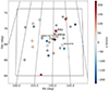 |
Fig. 1. Survey footprint from Chiboucas et al. (2009, 2013). The two main galaxies M 81 and M 82 are indicated as stars, the dwarf spheroidals are shown as dots, and the dwarf irregulars are plotted as squares. The two brightest satellites (NGC 2976 and NGC 3077) are marked. The colors indicate the observed velocities. Gray means that no velocity measurement is currently available. |
To study the flattening of the satellite distribution, we employed the Hough transformation as described in Heesters et al. (2021). In short, the Hough transform (Hough 1959, 1962) was originally developed as a tool for detecting straight lines and other simple shapes in digital images. The principle of the method is a voting system in which all points in an image decide on the best-fit parameters from a predefined set of slope and intercept pairs. For every data point, we defined a range of lines that cross the point from different directions. With these lines, the point votes for the best fit that should describe the overall linear distribution. Since the image space has no bounds for slope and intercept, the lines were transformed to the so-called Hough space via the relation
 (1)
(1)
Here, x and y are the coordinates of the data point in the image space. The parameter ρ is the orthogonal distance from the origin to the line passing through the data point. Finally, θ is the angle between the ρ vector and the x-axis. In this space, the parameter ranges are closed with θ ∈ [ − π/2, π/2] and ρ ∈ [ − d, d], where d is the diagonal of the image. The votes by each data point are generated by calculating the values for ρ corresponding to a range of θ values via Eq. (1). This process amounts to a dotted curve in the Hough space for every data point. Each of these dots represents one vote, that is, one line that passes through one of the data points. The region in the Hough space in which the highest number of these lines cross represents the parameters with the highest number of votes at the end of this process, optimally describing the data set at hand. In an ideal scenario, where all data points are arranged on a perfectly straight line, there is a single crossing point in this parameter space. For scattered data points, however, the curves no longer cross in a single point. For this case, we identified the region with the highest overdensity of crossing lines and adopted a variable search area, allowing us to probe different scales. We optimized the area such that the structure flatness and the number of voting members were maximized simultaneously. This method allows for an educated estimation of the members of a potentially correlated satellite structure, that is, a plane seen close to edge-on, in the absence of three-dimensional information. The success of the method has been demonstrated on the M31 system (Heesters et al. 2021), for which only about half of the satellites appear to be part of a phase-space correlation (Ibata et al. 2013). Details about this fitting technique can be found in Heesters et al. (2021).
3. Satellite distribution
In this section, we examine the spatial and kinematic distribution of the satellite system of M 81.
3.1. Planes of satellites
In Fig. 2 we present the 2D distribution of the galaxies in the M 81 group and the morphological types of the satellites. A simple total least-squares (TLS) fit of the satellite system in 2D reveals an axis ratio of b/a = 0.79 (semiminor axis b = 91 kpc, semimajor axis a = 115 kpc), but this approach does not consider the possibility that some outliers may not belong to a flattened structure, which artificially increases the b/a ratio. The Hough method identifies a significantly flattened structure along the diagonal of the field. Out of the 34 satellites, 30 follow this elongated structure. Of the 4 satellites (HS117, d1028+70, DDO82, d1042+70) that are not part of the structure, only one is a dwarf spheroidal (d1042+70). Removing these 4 outliers, we measure a minor-to-major axis ratio b/a = 0.50 (semiminor axis b = 61 kpc, semimajor axis a = 122 kpc), which is similar to what is found for Cen A (b/a ≈ 0.5, Müller et al. 2016), but spatially less flattened than the Local Group planes (we note that the Local Group planes are studied in 3D due to better distance and thus 3D position accuracy). It is also consistent with the rms width estimated by Chiboucas et al. (2013). When we repeat the steps (i.e., Hough transformation and removal of the outliers) for the dSph alone, we obtain b/a = 0.34 (semiminor axis b = 42 kpc, semimajor axis a = 124 kpc), with 16 out of 19 dSph belonging to the flattened structure. However, 2 dwarf galaxies, KK77 and F8D1, that were previously considered in the Hough fitting are now not found to be part of the flattened structure. This is interesting because F8D1 has a disrupted profile exhibiting a tidal tail (Žemaitis et al. 2023) that is aligned approximately along the minor axis of the flattened structure. When we consider this shape as a tracer of the motion of the dwarf, it is moving out from the planar structure. When we consider the entire dSph sample in a TLS fit, we measure an axis ratio of b/a = 0.62 (semiminor axis b = 73 kpc, semimajor axis a = 117 kpc). That the flattening is higher for the dSph population compared to the total population is in line with the finding of Chiboucas et al. (2013), who suggested that a flattened structure exists that consists of the dwarf spheroidals in the M 81 group.
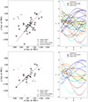 |
Fig. 2. Detecting linear structures with the Hough transform. Left: M81 group satellite system in relative coordinates, with M81 (star) at the origin and indicating projected separations at the distance of M 81 in kpc. M 82 is shown as an empty star. The dwarf satellites of different morphologies are shown as circles and squares. We emphasize the abundance of dwarf spheroidals (dSphs) as black circles compared to other morphologies as gray squares. The best-fit line is determined via the Hough method, which finds all but four satellites (upper left corner) to be members (circled gray) of a flattened structure. The rms dimensions of this structure are indicated with black arrows. Top: Results using all morphological types of satellites. Bottom: Only using the dSphs. Right: M 81 satellite system in the Hough parameter space. The parameter ρ plotted on the y-axis is the normal distance from the fit line to the origin, while θ is the angle between this ρ vector and the x-axis in the image space. Each curve corresponds to a series of possible parameter pairs for one dwarf. The curves are z-score normalized along each axis, i.e., they have a mean of zero and a standard deviation of one. The red dot indicates the parameter pair at the center of the densest crossing region (gray circle), which is optimized to maximize the number of structure members and the flatness of the system simultaneously. The curves that do not cross the gray region stem from the declared outliers in the scatter plot left. |
The orientation of the flattened structure with respect to the Local Universe is studied next. We examined how the flattened structure is aligned with respect to the surrounding large-scale matter distribution, as characterized by the velocity-shear tensor, specifically, its principle eigenvectors (e.g Hoffman et al. 2012). The eigenvector corresponding to the slowest collapse, ( ), defines the spines of cosmic filaments, whereas the axis of greatest compression (
 ) is associated with the normal of cosmic sheets (see Libeskind et al. 2018, and references therein). Libeskind et al. (2015, 2019) performed such an analysis of the known dwarf galaxy planes (i.e., MW, M31, and Centaurus A) in 3D using a quasi-linear reconstruction of the Local Universe from CF2 (Hoffman et al. 2018; Tully et al. 2013) and found that many of their normals tended to be closely aligned with
  , the eigenvectors of the shear tensor corresponding to the axis of greatest compression. To test whether the M 81 satellite population is aligned with any of these vectors, we can transformed the system into supergalactic coordinates (de Vaucouleurs 1956; Lahav et al. 1998). In the supergalactic coordinates, the Local Sheet, including the Local Group, NGC253, Cen A, and M 81, is aligned with the supergalactic SGX-SGY plane, which corresponds to the
  –
– plane. The satellite system in in 3D supergalactic coordinates is presented in Fig. 3. We studied the alignment of the satellite system with a principal component analysis (pca) using the Python package sklearn (Pedregosa et al. 2011). The pca method determines the eigenvectors of a data set. We used it to estimate the direction with the smallest variance, which for a flattened distribution of data points corresponds to its normal vector. When we consider all dwarfs, including the four outliers that we do not deem to be part of the plane of satellites, the normal for the planar structure in supergalactic coordinates is [−0.1314, +0.0374, +0.9906]. The normal including all dwarf galaxies in the flattened structure is [−0.0899, +0.0772, +0.9930]. The angle between the two normals is only 3 degrees, which means that they align well and can be regarded as equal. The position of the normal with respect to the shear tensor is given in Fig. 4.
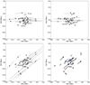 |
Fig. 3. Satellite system of M 81 in Cartesian supergalactic coordinates, shifted to the center of the satellite distribution. The dSphs are indicated as dark gray dots, the dIrr as squares in a lighter gray, and the main galaxies M 81 and M 82 as white stars. The thin black lines indicate the distance uncertainties. The top panels represent an edge-on view of the plane, and the bottom panels show a face-on view. In the bottom right panel, the velocities are indicated as thick lines, as well as the color. Red indicates galaxies moving away from us with respect to the mean velocity of the system, and blue indicates galaxies moving toward us. The color-coding is the same as in Fig. 5. |
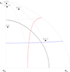 |
Fig. 4. Orientation of the poles of planes of satellites with respect to the surrounding large-scale matter distribution. The eigenvector |

The flattened satellite structure of M 81 has its normal aligned close to  of the velocity-shear tensor defined by the large-scale matter distribution in the Local Universe. This is consistent with Chiboucas et al. (2013), who noted an apparent flattening of the distribution of gas-deficient systems to the supergalactic equatorial plane. However, we note that employing the Hough transformation, we find both an alignment considering dSphs alone and dSphs and dIrrs together. The alignment of the M 81 satellite system with the Local Sheet also holds for the satellite systems of M 31 and Cen A (Libeskind et al. 2015, 2019). However, for the best-studied plane-of-satellite system, that is, around the Milky Way, no such alignment can be found. This may indicate that these structures have different origins.
It is interesting to note that the four dwarf galaxies (HS117, d1028+70, DDO82, and d1042+70) that are not part of the main structure form some kind of elongated spur as well, which extends parallel to the main structure. It has a minor-to-major axis ratio b/a = 0.28 (semiminor axis b = 13 kpc, semimajor axis a = 46 kpc). There is a gap of 222 kpc between the best-fitting plane from these four dwarfs and the main flattened structure. This gap is well visible in 2D in Fig. 1 and in 3D in Fig. 3.
3.2. Lopsidedness
Evidence for an asymmetric distribution of the satellite system can be studied using different metrics testing for lopsidedness in the group. We used two simple approaches: a) the distance of the centroid from M 81, and b) a hemisphere approach.
In the first approach, we tested whether the center of the satellite distribution coincided with the dominant galaxy M 81. We defined the center or centroid of the Hough fit as
 (2)
(2)
Here, N is the number of structure members, and ri are the member coordinates. The centers for the two Hough fit lines (using all dwarfs and only the dSph) are presented in Fig. 2. They are separated from each other by 23 kpc. The centroids for both samples are off from the position of M 81 by ≈40 kpc. To test whether this is significant, we ran a Monte Carlo simulation in which we generated for each iteration 30 random positions uniformely drawn within the box defined by the plane of satellites (i.e., with b = 61 kpc and a = 122 kpc). Finding the center of the point cloud for each iteration, we estimated that an offset of 40 kpc occurs in only 0.2% of the cases. In other words, it is significant at the 3σ level. This may indicate that the dwarf satellite population is not symmetrically distributed around M 81, which could be a physical effect caused by the ongoing interaction between M81, M82, and NGC3077. It might also arise from an infalling group of dwarfs (see the Sect. 3.3 for indications of this).
Another way to test lopsidedness is to split the distribution of the satellites into two hemipsheres. This lopsidedness has been found within the Local Group (Conn et al. 2013) and statistically in galaxy groups in the Sloan digital sky survey (SDSS, Libeskind et al. 2016). The study by Pawlowski et al. (2017) of these SDSS systems in ΛCDM cosmological simulations found that this anisotropy agrees with observations. Kanehisa et al. (2024) reported that the M31 satellite system lopsidedness significantly disagrees with ΛCDM simulation expectations, however. It is therefore interesting to determine whether we find this in the M 81 group. Taking the minor axis of the satellite distribution as a separation line, which we fixed at the position of M 81 (the brightest galaxy in the group), we find that 11 satellite galaxies are on one side and 23 on the other. Assuming a Bernouilli distribution for a satellite being on one side or another (i.e., a fair coin flip), we estimated that finding 11 or fewer satellites on one side has a probability of 5.8% (we have to consider two cases, i.e., finding 11 or fewer, and finding 23 or more in a Bernouilli experiment). This does not pass the 3σ threshold, and we therefore do not find it to be significant.
3.3. Kinematics
Velocity measurements are available for 19 dwarf galaxies, 16 of which are members of the reported flattened structure. This is comparable to available line-of-sight data for the Andromeda galaxy and Cen A. However, these galaxy groups are more simple in terms of their dynamics, because they are both dominated by a single giant galaxy. On the other hand, the M 81 group consists of at least two main galaxies, M 81 and M 82, and several massive dwarfs such as NGC 2976 and NGC 3077. This hampers an analysis of the dynamics of the group. For example, M 81 has a line-of-sight velocity of −38 km s−1 (Dickel & Rood 1978) and M 82 of 183 km s−1 (Appleton et al. 1981). The mean line-of-sight velocity of the satellites is 20 km s−1, which is offset by ≈60 km s−1 from the velocity of M 81. In comparison, the difference between the velocity of Cen A and the mean of its satellite system is 1 km s−1 (Müller et al. 2021). When we take a simple approach and use the mean satellite velocity of the dwarfs that are found to be part of the structure (29 km s−1) as an anchor, which coincides with the luminosity-weighted velocity of M 81/M 82 (29 km s−1), we can produce a position-velocity (PV) diagram for the flattened structure (see Fig. 5). In general, we expect that a fully corotating system would occupy two out of the four quadrants on opposing sides, and a fully pressure-supported system all four quadrants. For the M 81 system, no clear signal of corotation is obvious. The two opposing quadrants each populate 9 and 7 satellites, respectively. In this plot, we used the 2D center of the flattened dwarf system as found with the Hough fit as the zeropoint for the distance. Other choices may be made, for instance, either using M 81 as the center, or a weighted mean between M 81 and M 82. Using the stellar luminosities as a proxy for the latter, we find only a minor difference (11 kpc) to the position of M 81, which is negligible. If the center were fixed at M 81, most dwarf galaxies would populate the left two quadrants (it would shift the vertical line to the right in Fig. 5).
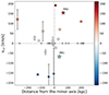 |
Fig. 5. Position-velocity diagram of the satellite system of the M 81 group. Blue denotes a satellite moving toward us, and red denotes a satellite moving away from us, relative to the mean group velocity (v = 29 km s−1). The gray symbols indicate the structure members without available line-of-sight velocities. The x-axis denotes the distance from the minor axis along the major axis. A negative sign on the distance is assigned based on their position on the left (positive x) of the minor axis. The circles highlight the dwarf spheroidals, and the squares show dwarfs of all other morphologies. The two stars indicate the two main galaxies M 81 and M 82. |
Assuming the flattened satellite system of M 81 is observed edge-on, we can study the line-of-sight velocities of the dwarfs from a face-on point of view of the system. This plot is presented in the bottom right panel of Fig. 3. The line-of-sight velocities are in the plane of this panel. There are a few interesting points to note. Almost all velocities come from dwarfs on one side, which coincides with the position of NGC 3077. Most of them are dIrrs. At least a few of these dwarfs might have been a distinct group including NGC 3077, and they might be falling in. Because the HI in dwarf galaxies is expected to be stripped when accreted by a massive galaxy such as M 81 (Spekkens et al. 2014), it is possible that we observe their (first) infall. Moreover, between M 81 and NGC 3077 lie five candidate tidal dwarf galaxies (d0959+68, BK3N, Garland, A0952+69, and Holm IX) that are embedded in the HI tidal material, so they may further complicate the dynamical interpretation of the system (see, e.g., Lelli et al. 2015 for bona fide tidal dwarf galaxies in other interacting systems). Out of these five candidates, all but d0959+68 have velocity measurements. Two would be comoving, as expected for a corotating plane of satellites, and two would be off. Tidal dwarf galaxies may offer a possible formation scenario for the creation of planes of satellites, with numerical flyby models showing that up to 50% of the tidal dwarf galaxies may end up on counter-rotating orbits (Pawlowski et al. 2011). However, without proper motion measurements for these dwarfs, we cannot assess whether they are truly co- or counter-rotating, only that they may be consistent with such a motion (see, e.g., Kanehisa et al. 2023b).
With the current incomplete picture of the satellite system (i.e., the missing velocities of half the dwarf galaxies), we cannot draw firm conclusions about the dynamical state of the system. There is currently no strong evidence for a corotation of the satellite system, however.
4. Comparison to Illustris-TNG50
To probe the significance of the flattened satellite distribution of M81, we used data from the IllustrisTNG suite (Pillepich et al. 2018; Nelson et al. 2019) of publicly available large-volume hydrodynamic simulations. It adopts cosmological parameters from Planck (Planck Collaboration XIII 2016): egaΛ = 0.6911, egam = 0.3089, and h = 0.6774. To best resolve the fainter dwarf population in the M81 group, we used the high-resolution TNG50-1 run, which spanned a simulation volume with a length of 51.7 Mpc, with dark and gas particle resolutions of MDM = 4.5 × 10⁵ M⊙ and Mgas = 8.5 × 10⁴ M⊙, respectively.
We defined the simulated M81 analogs as having a stellar mass between 5 × 10¹⁰ M⊙ and 2 × 10¹¹ M⊙ while also requiring an associated halo mass M200 between 5 × 10¹¹ M⊙ and 2 × 10¹² M⊙ (as motivated by the dynamical mass estimate for M81 of 1.17 × 10¹² M⊙ from Oehm et al. 2017). Analogs must also be isolated from other dwarf associations. We specifically rejected all systems with a companion halo 250 − 1000 kpc away with a halo mass above 0.25M200. This gives us our sample of M 81 analogs. Additionally, we inspected each M81 system analog for a corresponding M82 analog, defined as a subhalo within 200 kpc of the host galaxy with a stellar mass above 0.25 M*, M81, thus accommodating the M81-M82 stellar mass ratio of ≈0.43 (Karachentsev et al. 2013). In the first step, we analyzed the full analog sample. In the second step, we restricted the sample by only considering systems that also feature an M82 analog and repeated our analysis.
Each M81 analog was mock-observed from ten isotropically distributed directions with corresponding distances drawn from the M81 distance modulus of μ = 27.84 ± 0.09. Because the satellite population of M81 is complete within a projected 230 kpc radius to a limiting magnitude of −10 in the r band, we identified all subhalos within a projected radius of 250 kpc with a depth of 500 kpc with respect to their host galaxy. The subhalos were ranked by their stellar mass (and then by the dark mass when no stellar particles are available), and the 34 most massive were taken as the satellite sample of the simulation. Finally, distance errors were drawn from the observed M81 satellites and were randomly associated with the simulated satellites along the mock-observed line of sight.
In order to assess the prevalence of similarly flattened structures in simulations, we performed the described Hough fitting procedure on the 5530 (340 featuring an M82 analog) M81 analog systems. To do this, we used the same parameter search area as was found to optimize the flattening and the number of structure members in the observed M81 satellite system. We compared the flattening and the degree of kinematic correlation, that is, the number of corotating satellites. The Hough fitting rejects 0–12 outliers (compared to 4 for the observations). The mean number of rejected outliers is 4 (as is the number of observed rejected outliers), with a standard deviation of 1.8. We determined a potential correlation between the number of outliers and the axis ratio of the resulting structures. In general, we would expect that a smaller sample (i.e., more outliers) would lead to a flatter structure (Pawlowski et al. 2017). However, there is no such correlation when we compare the distributions of b/a ratios for the different samples with the outliers between 0 to 12. This is due to how we set up the search radius during the Hough fitting on the simulated systems. We required it to be the same as for the observed system (maximizing flatness and the number of objects considered in the fitting). If we were not to require this, we would indeed find a correlation between the thickness and the sample size.
Because not all satellites have available velocity measurements, we assessed the fraction of observed structure members that has such estimates (53%). When finding a linear substructure among the outliers, the Hough fitting technique is not forced to include the same number of satellites in the simulations that are found to be part of the structure (30). As discussed before, the method selects a variable number of dwarfs, which is very similar to the number of structure members in observations. Because the structure populations are slightly variable in every simulated analog system, we selected 53% of the velocities from the structure member satellites in the simulated systems. We used the satellites with the highest dark matter mass (as a proxy for their stellar mass) for this and used them to determine the fraction of corotating satellites along the major axis of a given structure. Similarly to the data analysis, we used the mean velocity of these satellites and the minor axis of their spatial distribution as anchor points for their corotation. The described comparison resulted in three measures of significance or p-values: the frequency of systems that match or exceed the observed axis radio, the degree of kinematic correlation, and the simultaneous occurrence of both properties. We find the corresponding p-values for the full sample and the sample featuring an M82 analog, respectively: pflat = 0.206 (0.294), pkin = 0.724 (0.735) and pboth = 0.151 (0.212). We thus estimate that the observed structure occurs in approximately 15.1% (21.2%) of M81-like systems. The results for both samples are illustrated in Fig. 6.
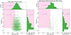 |
Fig. 6. Comparison of the M81 flattened-structure parameters with M81 analogs from TNG50. On the x-axis, we plot the short over long axis ratio (b/a), and on the y-axis, we plot the number of corotating satellites. The green crosses show the parameters of the M81 analogs in simulations, and the pink star shows the parameter pair of the data. The top histogram shows the distribution of the axis ratios of the structures around simulated analogs, and the histogram on the right shows the corresponding number of kinematically correlated dwarfs. The pink shaded regions illustrate the analog systems that match or exceed the parameters found in the data. The inset texts indicate the corresponding frequencies of these systems in simulations. Left: Results for all simulated M81 analogs. Right: Results for the subsample of analogs that also feature an M82 analog. |
Since not all M81 satellites have available velocity measurements at this time, the degree of corotation in the structure members is still unknown. Inspecting the structure members, we determined that the minimum number of possible corotating structure members is 15 (50%) and the maximum number is 23 (76.6%). In a second comparison between the data and the simulated systems, we considered the velocities of all structure members in simulations to determine the fraction of corotation. We studied all possible outcomes in terms of corotation given the missing velocities in the data and compared all possibilities with the expectations from the simulated analog systems. This resulted in a p-value for every possible fraction of corotation and allowed us to predict the number of satellites that is are expected to corotate so that this would be consistent with ΛCDM. The results of this comparison are illustrated in Fig. 7. The fractions of simulated systems for which both the flatness and degree of corotation match or exceed the possible values with future observations range from 2.1% to 29.4%. This illustrates that the consistency with the expectations from cosmological simulations is still uncertain because of the lacking velocities and therefore unknown degree of corotation in the reported structure.
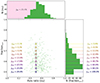 |
Fig. 7. Same as Fig. 6 (right), but illustrating the possible outcomes given lacking velocity measurements. The colored stars show the possible axis ratios and fractions of corotation in the data. The flatness of the structure will not change with new velocity information because distance measurements are available for all dwarfs. The fractions of corotation can vary from 0.5 (15/30) to 0.76 (23/30). For each possible scenario, the fraction of simulated systems that match or exceed the degree of kinematic correlation is shown in the histogram to the right. The fractions of systems that show both flatness and a degree of corotation similar to or more extreme than the data are shown in the center. |
5. Summary and conclusions
The plane-of-satellites problem has been identified as one of the greatest challenges to cosmology on small scales (Sales et al. 2022). Therefore, it is imperative to study different galaxy groups and test whether the motion and distribution of the satellite galaxies follows the predictions from cosmological simulations. In this work, we quantified previous claims of a flattened structure of dwarf galaxies in the compact M 81 group. We find that 30 out of 34 dwarf galaxies follow a flattened structure with a minor-to-major axis ratio of b/a = 0.5, which is similar to that of Cen A (Müller et al. 2019) and of early-type galaxies in the nearby universe (10–45 Mpc, Heesters et al. 2021) from the MATLAS survey (Habas et al. 2020; Poulain et al. 2021). When we consider only the dwarf spheroidals, the flattening increases to a ratio of 0.34. This is still thicker than the best-studied planes around the Milky Way and the Andromeda galaxy (c/a < 0.2). However, for the Milky Way and Andromeda systems, accurate distance estimates are available, so that the axis ratio can be estimated in 3D. Here, the thickness was measured in 2D. When the planar structure is significantly inclined with respect to the line of sight, the projected 2D thickness increases. The difference between the thickness of the dSph-only and the dSph+dIrr samples may also arise from the lower numbers of tracers. The fewer tracers, the more likely a thinner spatial distribution (Pawlowski et al. 2017).
We have compared the on-sky flattening and motion of the satellites in the M 81 group with TNG50 from the IllustrisTNG suite to determine how consistent the flattened structure is with cosmological predictions. In contrast to the Local Group and Centaurus system, we find agreement within 2σ with ΛCDM expectations. This is an interesting result because M 81 is in a different dynamical state than the Milky Way with its quiet merger history, and Andromeda and Cen A with putative major mergers 2–3 Gyr ago (Hammer et al. 2018; Wang et al. 2020).
Considering the possible coherent motion of satellites, which is the crucial property of satellite systems to test ΛCDM, we find no correlation for the M 81 satellites. This is in contrast to the Milky Way, the M 31, and Cen A satellites, which all seem to follow a coherent motion around their hosts. The reason for this is unclear.
The M 81 group is a compact group that is currently undergoing a major merger and is therefore not in dynamical equilibrium. This is evident from strong signs of interactions between M 81, M 82, and NGC3077, especially in HI (Chynoweth et al. 2008). Even if there was a corotating plane of satellites around M 81 before, an encounter like this may destroy any signs of corotation. Simulating the effect of major mergers on the creation or destruction of planes of satellites could help us understand the observations of the M 81 group. In this respect, simulations of the major merger of Cen A indicate a connection between the merger and the plane of satellites (Wang et al. 2020), but more detailed simulations are needed to reproduce the Cen A system. However, studies using TNG100 from the IllustrisTNG suite of cosmological simulations show a negligible contribution of the major merger history to the phase-space coherence of satellite galaxies (Kanehisa et al. 2023a). In this context, we would neither expect the formation nor destruction of a corotating satellite system around M 81.
Another explanation could be that we witness a mixing of several dwarf galaxy systems. A group of dwarf galaxies might be falling in together. This is indicated by the clustered distribution of dIrrs toward one side of M 81. In addition, at least 4 out of 19 satellites for which we have velocity information (d0952+69, BK3N, HolmIX, and Garland) are candidate tidal dwarf galaxies. They are embedded in the HI tidal material between M 81 and NGC 3077. Two of them reduce the phase-space signal. Before a coherent motion of satellites is ruled out, it is imperative to sample the full dwarf galaxy population around M 81, especially dwarf spheroidal galaxies, for which we can rule out a recent infall or a recent tidal formation. Fifteen more dwarf galaxies await velocity measurements, and many of them are dSphs, for which we find a more significant flattening than for the whole population. By studying the possible degrees of corotation in the reported flattened structure in light of the missing velocity measurements, we can predict the expected fraction of corotating satellites such that the observed structure is consistent with its simulated analogs. The fractions of simulated analogs that match or exceed both the observed flatness and kinematic correlation range from 2.1% to 29.4%. This indicates that the consistency with expectations from the most recent cosmological simulations is still uncertain until the lacking 15 velocity measurements are obtained.
Acknowledgments
We thank the referee for the constructive report, which helped to clarify and improve the manuscript. O.M. and N.H. are grateful to the Swiss National Science Foundation for financial support under the grant number PZ00P2_202104. M.S.P. acknowledges funding of a Leibniz-Junior Research Group (project number J94/2020) and a KT Boost Fund by the German Scholars Organization and Klaus Tschira Stiftung.
References
- Appleton, P. N., Davies, R. D., & Stephenson, R. J. 1981, MNRAS, 195, 327 [NASA ADS] [CrossRef] [Google Scholar]
- Bell, E. F., Smercina, A., Price, P. A., et al. 2022, ApJ, 937, L3 [NASA ADS] [CrossRef] [Google Scholar]
- Cautun, M., Bose, S., Frenk, C. S., et al. 2015, MNRAS, 452, 3838 [NASA ADS] [CrossRef] [Google Scholar]
- Chiboucas, K., Karachentsev, I. D., & Tully, R. B. 2009, AJ, 137, 3009 [Google Scholar]
- Chiboucas, K., Jacobs, B. A., Tully, R. B., & Karachentsev, I. D. 2013, AJ, 146, 126 [Google Scholar]
- Chynoweth, K. M., Langston, G. I., Yun, M. S., et al. 2008, AJ, 135, 1983 [NASA ADS] [CrossRef] [Google Scholar]
- Conn, A. R., Lewis, G. F., Ibata, R. A., et al. 2013, ApJ, 766, 120 [NASA ADS] [CrossRef] [Google Scholar]
- Dalcanton, J. J., Williams, B. F., Seth, A. C., et al. 2009, ApJS, 183, 67 [Google Scholar]
- de Vaucouleurs, G. 1956, Vistas Astron., 2, 1584 [NASA ADS] [CrossRef] [Google Scholar]
- Dickel, J. R., & Rood, H. J. 1978, ApJ, 223, 391 [NASA ADS] [CrossRef] [Google Scholar]
- Ferrarese, L., Ford, H. C., Huchra, J., et al. 2000, ApJS, 128, 431 [Google Scholar]
- Habas, R., Marleau, F. R., Duc, P.-A., et al. 2020, MNRAS, 491, 1901 [NASA ADS] [Google Scholar]
- Hammer, F., Yang, Y. B., Wang, J. L., et al. 2018, MNRAS, 475, 2754 [NASA ADS] [Google Scholar]
- Heesters, N., Habas, R., Marleau, F. R., et al. 2021, A&A, 654, A161 [NASA ADS] [CrossRef] [EDP Sciences] [Google Scholar]
- Hoffman, Y., Metuki, O., Yepes, G., et al. 2012, MNRAS, 425, 2049 [Google Scholar]
- Hoffman, Y., Carlesi, E., Pomarède, D., et al. 2018, Nat. Astron., 2, 680 [NASA ADS] [CrossRef] [Google Scholar]
- Hough, P. V. 1959, Conf. Proc., 590914, 554 [Google Scholar]
- Hough, P. V. 1962, Method and means for recognizing complex patterns, (US Atomic Energy Commission) [Google Scholar]
- Huchtmeier, W. K., Karachentsev, I. D., & Karachentseva, V. E. 2003, A&A, 401, 483 [CrossRef] [EDP Sciences] [Google Scholar]
- Ibata, R. A., Lewis, G. F., Conn, A. R., et al. 2013, Nature, 493, 62 [NASA ADS] [CrossRef] [Google Scholar]
- Ibata, N. G., Ibata, R. A., Famaey, B., & Lewis, G. F. 2014a, Nature, 511, 563 [CrossRef] [Google Scholar]
- Ibata, R. A., Ibata, N. G., Lewis, G. F., et al. 2014b, ApJ, 784, L6 [NASA ADS] [CrossRef] [Google Scholar]
- Kanehisa, K. J., Pawlowski, M. S., & Müller, O. 2023a, MNRAS, 524, 952 [NASA ADS] [CrossRef] [Google Scholar]
- Kanehisa, K. J., Pawlowski, M. S., Müller, O., & Sohn, S. T. 2023b, MNRAS, 519, 6184 [NASA ADS] [CrossRef] [Google Scholar]
- Kanehisa, K. J., Pawlowski, M. S., et al. 2024, Nat. Astron., submitted [Google Scholar]
- Karachentsev, I. D., & Kashibadze, O. G. 2005, arXiv e-prints [arXiv:astro-ph/0509207] [Google Scholar]
- Karachentsev, I. D., & Kroupa, P. 2024, MNRAS, 528, 2805 [NASA ADS] [CrossRef] [Google Scholar]
- Karachentsev, I. D., Karachentseva, V. E., & Boerngen, F. 1985, MNRAS, 217, 731 [NASA ADS] [CrossRef] [Google Scholar]
- Karachentsev, I. D., Karachentseva, V. E., Dolphin, A. E., et al. 2000, A&A, 363, 117 [NASA ADS] [Google Scholar]
- Karachentsev, I. D., Sharina, M. E., Dolphin, A. E., et al. 2001, A&A, 375, 359 [NASA ADS] [CrossRef] [EDP Sciences] [Google Scholar]
- Karachentsev, I. D., Dolphin, A. E., Geisler, D., et al. 2002, A&A, 383, 125 [CrossRef] [EDP Sciences] [Google Scholar]
- Karachentsev, I. D., Makarov, D. I., Sharina, M. E., et al. 2003, A&A, 398, 479 [NASA ADS] [CrossRef] [EDP Sciences] [Google Scholar]
- Karachentsev, I. D., Karachentseva, V. E., Huchtmeier, W. K., & Makarov, D. I. 2004, AJ, 127, 2031 [Google Scholar]
- Karachentsev, I. D., Dolphin, A., Tully, R. B., et al. 2006, AJ, 131, 1361 [Google Scholar]
- Karachentsev, I. D., Makarov, D. I., & Kaisina, E. I. 2013, AJ, 145, 101 [Google Scholar]
- Koch, A., & Grebel, E. K. 2006, AJ, 131, 1405 [NASA ADS] [CrossRef] [Google Scholar]
- Kroupa, P., Theis, C., & Boily, C. M. 2005, A&A, 431, 517 [NASA ADS] [CrossRef] [EDP Sciences] [Google Scholar]
- Lahav, O., Santiago, B. X., Webster, A. M., et al. 1998, arXiv e-prints [arXiv:astro-ph/9809343] [Google Scholar]
- Lang, R. H., Boyce, P. J., Kilborn, V. A., et al. 2003, MNRAS, 342, 738 [NASA ADS] [CrossRef] [Google Scholar]
- Lelli, F., Duc, P.-A., Brinks, E., et al. 2015, A&A, 584, A113 [NASA ADS] [CrossRef] [EDP Sciences] [Google Scholar]
- Libeskind, N. I., Frenk, C. S., Cole, S., et al. 2005, MNRAS, 363, 146 [NASA ADS] [CrossRef] [Google Scholar]
- Libeskind, N. I., Cole, S., Frenk, C. S., Okamoto, T., & Jenkins, A. 2007, MNRAS, 374, 16 [NASA ADS] [CrossRef] [Google Scholar]
- Libeskind, N. I., Hoffman, Y., Tully, R. B., et al. 2015, MNRAS, 452, 1052 [NASA ADS] [CrossRef] [Google Scholar]
- Libeskind, N. I., Guo, Q., Tempel, E., & Ibata, R. 2016, ApJ, 830, 121 [NASA ADS] [CrossRef] [Google Scholar]
- Libeskind, N. I., van de Weygaert, R., Cautun, M., et al. 2018, MNRAS, 473, 1195 [NASA ADS] [CrossRef] [Google Scholar]
- Libeskind, N. I., Carlesi, E., Müller, O., et al. 2019, MNRAS, 490, 3786 [NASA ADS] [CrossRef] [Google Scholar]
- Lynden-Bell, D. 1976, MNRAS, 174, 695 [NASA ADS] [Google Scholar]
- Makarov, D. I., Karachentsev, I. D., & Burenkov, A. N. 2003, A&A, 405, 951 [NASA ADS] [CrossRef] [EDP Sciences] [Google Scholar]
- Makarova, L., Koleva, M., Makarov, D., & Prugniel, P. 2010, MNRAS, 406, 1152 [NASA ADS] [Google Scholar]
- Martínez-Delgado, D., Makarov, D., Javanmardi, B., et al. 2021, A&A, 652, A48 [NASA ADS] [CrossRef] [EDP Sciences] [Google Scholar]
- McConnachie, A. W., & Irwin, M. J. 2006, MNRAS, 365, 902 [CrossRef] [Google Scholar]
- Metz, M., Kroupa, P., & Libeskind, N. I. 2008, ApJ, 680, 287 [NASA ADS] [CrossRef] [Google Scholar]
- Müller, O., Jerjen, H., Pawlowski, M. S., & Binggeli, B. 2016, A&A, 595, A119 [NASA ADS] [CrossRef] [EDP Sciences] [Google Scholar]
- Müller, O., Scalera, R., Binggeli, B., & Jerjen, H. 2017, A&A, 602, A119 [NASA ADS] [CrossRef] [EDP Sciences] [Google Scholar]
- Müller, O., Pawlowski, M. S., Jerjen, H., & Lelli, F. 2018a, Science, 359, 534 [CrossRef] [Google Scholar]
- Müller, O., Rejkuba, M., & Jerjen, H. 2018b, A&A, 615, A96 [NASA ADS] [CrossRef] [EDP Sciences] [Google Scholar]
- Müller, O., Rejkuba, M., Pawlowski, M. S., et al. 2019, A&A, 629, A18 [Google Scholar]
- Müller, O., Pawlowski, M. S., Lelli, F., et al. 2021, A&A, 645, L5 [NASA ADS] [CrossRef] [EDP Sciences] [Google Scholar]
- Nelson, D., Springel, V., Pillepich, A., et al. 2019, Comput. Astrophys. Cosmol., 6, 2 [Google Scholar]
- Oehm, W., Thies, I., & Kroupa, P. 2017, MNRAS, 467, 273 [NASA ADS] [Google Scholar]
- Okamoto, S., Arimoto, N., Ferguson, A. M. N., et al. 2015, ApJ, 809, L1 [NASA ADS] [CrossRef] [Google Scholar]
- Okamoto, S., Arimoto, N., Ferguson, A. M. N., et al. 2019, ApJ, 884, 128 [NASA ADS] [CrossRef] [Google Scholar]
- Paudel, S., Yoon, S.-J., & Smith, R. 2021, ApJ, 917, L18 [NASA ADS] [CrossRef] [Google Scholar]
- Pawlowski, M. S. 2018, Mod. Phys. Lett. A, 33, 1830004 [NASA ADS] [CrossRef] [Google Scholar]
- Pawlowski, M. S. 2021, Nat. Astron., 5, 1185 [NASA ADS] [CrossRef] [Google Scholar]
- Pawlowski, M. S., & Kroupa, P. 2020, MNRAS, 491, 3042 [NASA ADS] [CrossRef] [Google Scholar]
- Pawlowski, M. S., Kroupa, P., & de Boer, K. S. 2011, A&A, 532, A118 [NASA ADS] [CrossRef] [EDP Sciences] [Google Scholar]
- Pawlowski, M. S., Pflamm-Altenburg, J., & Kroupa, P. 2012, MNRAS, 423, 1109 [NASA ADS] [CrossRef] [Google Scholar]
- Pawlowski, M. S., Ibata, R. A., & Bullock, J. S. 2017, ApJ, 850, 132 [NASA ADS] [CrossRef] [Google Scholar]
- Pedregosa, F., Varoquaux, G., Gramfort, A., et al. 2011, J. Mach. Learn. Res., 12, 2825 [Google Scholar]
- Pillepich, A., Springel, V., Nelson, D., et al. 2018, MNRAS, 473, 4077 [Google Scholar]
- Planck Collaboration XIII. 2016, A&A, 594, A13 [NASA ADS] [CrossRef] [EDP Sciences] [Google Scholar]
- Poulain, M., Marleau, F. R., Habas, R., et al. 2021, MNRAS, 506, 5494 [NASA ADS] [CrossRef] [Google Scholar]
- Sales, L. V., Wetzel, A., & Fattahi, A. 2022, Nat. Astron., 6, 897 [NASA ADS] [CrossRef] [Google Scholar]
- Sawala, T., Cautun, M., Frenk, C., et al. 2023, Nat. Astron., 7, 481 [Google Scholar]
- Sharina, M. E., Karachentsev, I. D., & Burenkov, A. N. 2001, A&A, 380, 435 [NASA ADS] [CrossRef] [EDP Sciences] [Google Scholar]
- Spekkens, K., Urbancic, N., Mason, B. S., Willman, B., & Aguirre, J. E. 2014, ApJ, 795, L5 [NASA ADS] [CrossRef] [Google Scholar]
- Taibi, S., Pawlowski, M. S., Khoperskov, S., Steinmetz, M., & Libeskind, N. I. 2024, A&A, 681, A73 [NASA ADS] [CrossRef] [EDP Sciences] [Google Scholar]
- Tikhonov, N. A., & Karachentsev, I. D. 1993, A&A, 275, 39 [NASA ADS] [Google Scholar]
- Tully, R. B., Courtois, H. M., Dolphin, A. E., et al. 2013, AJ, 146, 86 [NASA ADS] [CrossRef] [Google Scholar]
- Tully, R. B., Libeskind, N. I., Karachentsev, I. D., et al. 2015, ApJ, 802, L25 [Google Scholar]
- Wang, J., Hammer, F., Rejkuba, M., Crnojević, D., & Yang, Y. 2020, MNRAS, 498, 2766 [NASA ADS] [CrossRef] [Google Scholar]
- Weisz, D. R., Skillman, E. D., Cannon, J. M., et al. 2008, ApJ, 689, 160 [NASA ADS] [CrossRef] [Google Scholar]
- Yun, M. S., Ho, P. T. P., & Lo, K. Y. 1994, Nature, 372, 530 [NASA ADS] [CrossRef] [Google Scholar]
- Žemaitis, R., Ferguson, A. M. N., Okamoto, S., et al. 2023, MNRAS, 518, 2497 [Google Scholar]
Appendix A: The data of the M81 satellite system
In Table A.1 we provide the properties of the dwarf galaxies used in this work.
M81 satellite system.
All Tables
All Figures
|
Fig. 1. Survey footprint from Chiboucas et al. (2009, 2013). The two main galaxies M 81 and M 82 are indicated as stars, the dwarf spheroidals are shown as dots, and the dwarf irregulars are plotted as squares. The two brightest satellites (NGC 2976 and NGC 3077) are marked. The colors indicate the observed velocities. Gray means that no velocity measurement is currently available. |
| In the text | |
|
Fig. 2. Detecting linear structures with the Hough transform. Left: M81 group satellite system in relative coordinates, with M81 (star) at the origin and indicating projected separations at the distance of M 81 in kpc. M 82 is shown as an empty star. The dwarf satellites of different morphologies are shown as circles and squares. We emphasize the abundance of dwarf spheroidals (dSphs) as black circles compared to other morphologies as gray squares. The best-fit line is determined via the Hough method, which finds all but four satellites (upper left corner) to be members (circled gray) of a flattened structure. The rms dimensions of this structure are indicated with black arrows. Top: Results using all morphological types of satellites. Bottom: Only using the dSphs. Right: M 81 satellite system in the Hough parameter space. The parameter ρ plotted on the y-axis is the normal distance from the fit line to the origin, while θ is the angle between this ρ vector and the x-axis in the image space. Each curve corresponds to a series of possible parameter pairs for one dwarf. The curves are z-score normalized along each axis, i.e., they have a mean of zero and a standard deviation of one. The red dot indicates the parameter pair at the center of the densest crossing region (gray circle), which is optimized to maximize the number of structure members and the flatness of the system simultaneously. The curves that do not cross the gray region stem from the declared outliers in the scatter plot left. |
| In the text | |
|
Fig. 3. Satellite system of M 81 in Cartesian supergalactic coordinates, shifted to the center of the satellite distribution. The dSphs are indicated as dark gray dots, the dIrr as squares in a lighter gray, and the main galaxies M 81 and M 82 as white stars. The thin black lines indicate the distance uncertainties. The top panels represent an edge-on view of the plane, and the bottom panels show a face-on view. In the bottom right panel, the velocities are indicated as thick lines, as well as the color. Red indicates galaxies moving away from us with respect to the mean velocity of the system, and blue indicates galaxies moving toward us. The color-coding is the same as in Fig. 5. |
| In the text | |
|
Fig. 4. Orientation of the poles of planes of satellites with respect to the surrounding large-scale matter distribution. The eigenvector |
| In the text | |
|
Fig. 5. Position-velocity diagram of the satellite system of the M 81 group. Blue denotes a satellite moving toward us, and red denotes a satellite moving away from us, relative to the mean group velocity (v = 29 km s−1). The gray symbols indicate the structure members without available line-of-sight velocities. The x-axis denotes the distance from the minor axis along the major axis. A negative sign on the distance is assigned based on their position on the left (positive x) of the minor axis. The circles highlight the dwarf spheroidals, and the squares show dwarfs of all other morphologies. The two stars indicate the two main galaxies M 81 and M 82. |
| In the text | |
|
Fig. 6. Comparison of the M81 flattened-structure parameters with M81 analogs from TNG50. On the x-axis, we plot the short over long axis ratio (b/a), and on the y-axis, we plot the number of corotating satellites. The green crosses show the parameters of the M81 analogs in simulations, and the pink star shows the parameter pair of the data. The top histogram shows the distribution of the axis ratios of the structures around simulated analogs, and the histogram on the right shows the corresponding number of kinematically correlated dwarfs. The pink shaded regions illustrate the analog systems that match or exceed the parameters found in the data. The inset texts indicate the corresponding frequencies of these systems in simulations. Left: Results for all simulated M81 analogs. Right: Results for the subsample of analogs that also feature an M82 analog. |
| In the text | |
|
Fig. 7. Same as Fig. 6 (right), but illustrating the possible outcomes given lacking velocity measurements. The colored stars show the possible axis ratios and fractions of corotation in the data. The flatness of the structure will not change with new velocity information because distance measurements are available for all dwarfs. The fractions of corotation can vary from 0.5 (15/30) to 0.76 (23/30). For each possible scenario, the fraction of simulated systems that match or exceed the degree of kinematic correlation is shown in the histogram to the right. The fractions of systems that show both flatness and a degree of corotation similar to or more extreme than the data are shown in the center. |
| In the text | |
Current usage metrics show cumulative count of Article Views (full-text article views including HTML views, PDF and ePub downloads, according to the available data) and Abstracts Views on Vision4Press platform.
Data correspond to usage on the plateform after 2015. The current usage metrics is available 48-96 hours after online publication and is updated daily on week days.
Initial download of the metrics may take a while.